A neural network for long-term super-resolution imaging of live cells with reliable confidence quantification
Main
The increase in spatial resolution with super-resolution (SR) microscopy is accompanied by the trade-offs with other imaging metrics such as speed and duration1,2. Recent advancements in deep neural networks have demonstrated remarkable capability to transform low-resolution (LR) images to their SR counterparts, thereby enabling instant single-image SR (SISR) without any modifications on optical setups and realizing ultralong-term live-cell SR imaging3,4,5,6,7,8,9,10,11,12. Nevertheless, there are two major limitations in existing SISR neural networks when applied to time-lapse data. Firstly, when applied to process time-lapse images, SISR models cannot capture the temporal dependencies between adjacent frames, thus yielding inferior SR fidelity and temporally inconsistent inferences5. Secondly, existing SISR models only generate monochromatic intensity images of biological structures without providing a quantitative and reliable evaluation on output confidence13, which makes it hard to trust the outputs14. These two defects severely impede the wide applications of SR neural networks in routine biological imaging experiments.
To address the aforementioned challenges, we first used our home-built multimodality structured illumination microscopy (Multi-SIM) system to acquire a large-scale high-quality dataset for the biological time-lapse image SR (TISR) task, named BioTISR. The BioTISR dataset contains thousands of well-matched LR–SR time-lapse image stacks with three different input signal-to-noise ratios (SNRs) and five biological specimens, allowing us to systematically evaluate state-of-the-art (SOTA) TISR neural networks. Instead of assessing numerous TISR models individually, we investigated the two most essential parts of the TISR network architecture, temporal information propagation and neighbor feature alignment, using a custom-designed general TISR framework. During the evaluation, we found that existing mainstream feature alignment mechanisms such as optical flow (OF)15 cannot always perform correct alignment speculatively because of the rapid motion of biological structures with global inconsistency and the intrinsic photon noise in fluorescent images (Supplementary Fig. 1). To this end, inspired by the frequency shifting property of Fourier transform (that is, the spatial shifting of structures is equal to phase changes in the Fourier domain), we devised a deformable phase-space alignment (DPA) mechanism that is able to adaptively learn large and tiny motions in the phase space at subpixel precision. Furthermore, resorting to the strong feature alignment capability of DPA, we propose the DPA-based TISR (DPA-TISR) model and demonstrate that DPA-TISR outperforms other SOTA TISR models in terms of both fidelity and temporal consistency.
To conquer the second issue, we incorporated Bayesian deep learning16 and a Monte Carlo dropout approach17 with the DPA-TISR neural network, dubbed Bayesian DPA-TISR, to characterize the aleatoric uncertainty and epistemic uncertainty16, respectively. By calculating local integration of the mixed probability distribution function (PDF) for each pixel (Methods), confidence maps that quantitatively evaluate the reliability of the output images could be generated. However, both our results and previous studies indicate that deep neural networks tend to be overconfident18 (that is, the predicted confidence is higher than the real one). To cope with this issue, we developed an iterative fine-tuning framework to minimize the expected calibration error (ECE), where the ECE is defined as the weighted average of the absolute differences of inference accuracy and confidence, which can be reduced more than fivefold with our methods. We demonstrate that DPA-TISR and Bayesian DPA-TISR enable low-cost SR live imaging with ultrahigh spatiotemporal resolution, extended duration and reliable confidence evaluation by visualizing and analyzing various intracellular organelle interactions in live cells.
Results
Evaluation of essential components for TISR neural networks
TISR or video SR (VSR) neural network models are designed to leverage temporal neighbor frames to assist the SR of the current frame and are, therefore, expected to achieve better performance than SISR models19 (Supplementary Note 1). Although TISR models have been widely explored in natural image SR to improve video definition, whether such models can be applied to super-resolve biological images (that is, enhancing both sampling rate and optical resolution) has been poorly investigated. Here, we used the total internal reflection fluorescence (TIRF) SIM, grazing incidence (GI) SIM and nonlinear SIM20 modes of our home-built Multi-SIM system to acquire an extensive TISR dataset of five different biological structures: clathrin-coated pits (CCPs), lysosomes, outer mitochondrial membranes (Mitos), microtubules (MTs) and F-actin filaments (Extended Data Fig. 1). For each type of specimen, we generally acquired over 50 sets of raw SIM images with 20 consecutive time points at 2–4 levels of excitation light intensity (Methods). Each set of raw SIM images was averaged out to a diffraction-limited wide-field (WF) image sequence and was used as the network input, while the raw SIM images acquired at the highest excitation level were reconstructed into SR-SIM images as the ground truth (GT) used in network training. In particular, the image acquisition configuration was modified into a special running order where each illumination pattern is applied 2–4 times at escalating excitation light intensity before changing to the next phase or orientation, so as to minimize the motion-induced difference between WF inputs and SR-SIM targets.
To effectively use the temporal continuity of time-lapse data, SOTA TISR neural networks consist of mainly two important components21,22: temporal information propagation and neighbor feature alignment. We selected two popular types of propagation approaches, sliding window (Fig. 1a) and recurrent network (Fig. 1b), and three representative neighbor feature alignment mechanisms, explicit warping using OF15 (Fig. 1c) and implicit alignment by nonlocal attention23,24 (NA; Fig. 1d) or deformable convolution21,25,26 (DC; Fig. 1e), resulting in six combinations in total. For fair comparison, we custom-designed a general TISR network architecture composed of a feature extraction module, a propagation and alignment module and a reconstruction module (Extended Data Fig. 2) and kept the architecture of the feature extraction module and reconstruction module unchanged while only modifying the propagation and alignment module during evaluation (Methods). We then examined the six models on five different data types: linear SIM data of MTs, lysosomes and Mito, three of the most common biological structures in live-cell experiments, nonlinear SIM data of F-actin, which is of the highest structural complexity and upscaling factor in BioTISR, and simulated data of tubular structure with infallible GT references (Supplementary Note 2). As is shown in Fig. 1f, Extended Data Fig. 3 and Supplementary Fig. 2, all models denoised and sharpened the input noisy WF image evidently, among which the model constructed with a recurrent scheme and DC alignment resolved the finest details compared to the GT-SIM image (indicated by white arrows in Fig. 1f). Furthermore, we calculated time-lapse correlation matrices (Fig. 1g) and image fidelity metrics (Fig. 1h–j) (that is, peak SNR (PSNR) and structural similarity (SSIM)) for the output SR images to quantitatively evaluate the temporal consistency and reconstruction fidelity, respectively. According to the evaluation, we found that (1) recurrent network-based propagation (RNP) outperformed sliding window-based propagation (SWP) in both temporal consistency and image fidelity with fewer trainable parameters (Methods) and (2) propagation mechanisms had little effect on the temporal consistency of the reconstructed SR time-lapse data, while the DC-based alignment generally surpassed the other two mechanisms with a similar number of parameters for all types of datasets (Supplementary Fig. 3).
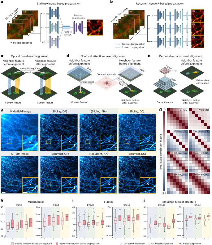
a,b, Schematic illustration of two temporal information propagation mechanisms: SWP (sliding; a) and RNP (recurrent; b). concat., concatenate. c–e, Schematic illustration of three neighbor feature alignment mechanisms using OF (c), NA (d) and DC (e). conv, convolution. f, Representative TISR MT images inferred by six models combining two propagation methods (sliding and recurrent) and three alignment mechanisms (OF, NA and DC). WF and GT-SIM images are shown in the first column for reference. g, Time-lapse correlation matrices of TISR images inferred by the models evaluated. h–j, Statistical comparison of the six models in terms of PSNR and SSIM on F-actin (h; n = 50), MTs (i; n = 50) and simulated tubular structures (j; n = 200). Center line, medians; limits, 75th and 25th percentiles; whiskers, the larger value between the largest data point and the 75th percentile plus 1.5× the IQR and the smaller value between the smallest data point and the 25th percentile minus 1.5× the IQR; outliers, data points larger than the upper whisker or smaller than the lower whisker. Scale bars, 3 μm (f) and 1 μm (zoomed-in regions in f).
Source data
Moreover, we validated these findings by using the simulated dataset under different dynamic and noise conditions (that is, structures with larger or smaller displacement between adjacent frames and higher or lower input SNR), with all experiments presenting similar results (Supplementary Figs. 4–7). We speculate that the underlying reasons are threefold: (1) the bidirectional and recurrent propagation allows the TISR model to learn longer-range dependencies and maximizes the temporal information gathering compared to the sliding window with a limited size; (2) biological images contain heavier photon noises and more rapid changes between adjacent frames than natural images, which greatly interferes with the accuracy of OF calculation, leading to adverse impact for the OF-based alignment; and (3) the NA-based alignment mainly mixes up the information from spatially and temporally neighboring pixels without modeling subpixel changes. In contrast, the DC-based alignment consists of both explicit subpixel shift estimation and implicit feature refinement, yielding the best capability to handle the complex motion pattern and spatially diverse speed for biological structures.
DPA mechanism for TISR
On the basis of our comprehensive evaluation of the SOTA methods, a strong baseline, which is a combination of RNP and DC-based alignment, has been well established. However, the existing DC mechanism only aggregates local features26 and fails to model global information and spatially consistent motion of biological structures. To this end, we further devised a DPA mechanism to enhance the global feature alignment at subpixel precision (Supplementary Note 3). In contrast to existing DC alignment, which estimates offset in the spatial space, the proposed DPA primarily works in frequential space to adaptively learn phase residuals (Fig. 2a and Methods), which corresponds to inflicting subpixel spatial shifting for each frequency component. By visualizing the features before and after phase-space alignment, we show that the phase-space alignment is able to fully exploit global dependencies to subtly model and compensate for the movement of biological structures (Fig. 2b). Afterward, we incorporated the superior feature alignment capability of DPA with the optimal TISR baseline model derived from the systematic evaluation to propose the DPA-TISR neural network, as shown in Extended Data Fig. 4.

a, Schematic of the DPA mechanism. b, Visualization of representative features before and after phase-space alignment, which indicates that the phase-space alignment is able to implicitly model and compensate for the subtle movement of structures as designed. c, Comparison of SR images of MTs inferred by VRT, BasicVSR++, DPA-TISR and a modified SISR model from DPA-TISR (Methods). WF and GT-SIM images are shown in the first column for reference. d, Correlation matrices of SR time-lapse images inferred by the SISR model and DPA-TISR. e,f, Statistical comparison of VRT, BasicVSR++, DPA-TISR and the modified SISR model in terms of PSNR (e) and SSIM (f) (n = 50). Center line, medians; limits, 75th and 25th percentiles; whiskers, the larger value between the largest data point and the 75th percentile plus 1.5× the IQR and the smaller value between the smallest data point and the 25th percentile minus 1.5× the IQR; outliers, data points larger than the upper whisker or smaller than the lower whisker. Scale bars, 3 μm (c) and 1 μm (zoomed-in regions in c).
Source data
To test whether DPA outperforms the conventional spatial deformable alignment (DA) mechanism, we replaced the DPA with DA and two other variants of phase-space alignment (that is, amplitude convolution and phase–amplitude convolution) in DPA-TISR (Supplementary Note 3). We found that the DPA with only phase convolution generally provided higher SR reconstruction fidelity in terms of PSNR and SSIM for both experimental and simulated datasets than other methods under similar computation complexity (Extended Data Fig. 5). Next, we compared the proposed DPA-TISR to two representative SOTA TISR models (that is, BasicVSR++ (ref. 21), a superior baseline model combining the recurrent propagation and DC alignment, and VRT27, a recently published video restoration transformer that uses self-attention28 to model long-range temporal dependency) and an SISR variant of DPA-TISR (Methods) for biological TISR. As shown in Fig. 2c–f, compared to TISR models, the SISR model failed to gather cross-frame information, thereby presenting inferior noise robustness and output temporal consistency (Supplementary Fig. 8). Among three TISR models, with all aforementioned advances, DPA-TISR better reconstructed finer details even in regions with severe noise and background fluorescence compared to BasicVSR++ and VRT (Fig. 2c) and achieved the highest PSNR and SSIM (Fig. 2e,f).
Next, we evaluated the performance of DPA-TISR models when they were applied to unseen data of different organelles, cell types and imaging modalities (Supplementary Note 4). Despite being trained with only the F-actin dataset acquired from COS-7 cells by TIRF-SIM, the DPA-TISR model could generally give reasonable SR inference for most of the fine biological structures for different types of testing data (Supplementary Figs. 9–11). However, there might exist undesired blur or wrong predictions because of the domain gap between training and testing data. Such a domain gap could be sufficiently eliminated by transfer learning with a moderate amount of training data and fine-tuning iterations, which demonstrates the adaptation and generalization capability of DPA-TISR (Supplementary Note 4).
Additionally, we demonstrate that the DPA scheme and DPA-TISR model can be extended for SR-SIM reconstruction (that is, adopting time-lapse raw SIM images instead of WF images as inputs) (Extended Data Fig. 6 and Supplementary Fig. 12a) and SR inference for time-lapse volumetric data (Extended Data Fig. 7 and Supplementary Fig. 12b), which substantially outperform SISR models in both tasks of SR-SIM reconstruction and volumetric SR inference for diverse biological specimens by effectively using the temporal continuity of data (Supplementary Note 5).
Rapid, long-term, SR live-cell imaging enabled by DPA-TISR
A great diversity of subcellular structures incessantly execute elaborate bioprocesses in living cells, among which F-actin cytoskeleton serves as a critical regulator of organelle positioning29 and is involved in various important cell functionalities such as clathrin-mediated endocytosis (CME)30. However, because of the extremely structural complexity of F-actin filaments, conventional SR live imaging methods have to impose relatively high excitation laser power to obtain enough fluorescence required by SR reconstruction; thus, the multicolor SR observation of F-actin and other organelles is usually limited to ~400 time points even when assisted by SOTA deep learning-based methods5. To test whether DPA-TISR is competent in the TISR live-cell imaging task under relatively critical imaging conditions, we trained two independent DPA-TISR models for F-actin and CCPs using corresponding datasets in BioTISR and applied them to characterize the fast and subtle dynamics of F-actin filaments and CCPs from noisy time-lapse TIRF images. As shown in Fig. 3a, although the noisy images were acquired using tenfold lower excitation laser power than routine TIFR experiments, DPA-TISR successfully resolved densely interlaced F-actin filaments and ring structures of CCPs, which achieved better resolution than the widely used hardware-based SR system AiryScan (Supplementary Fig. 13 and Supplementary Note 6) and yielded an extended SR observation window of 4,800 time points (Supplementary Video 1). Benefiting from the well-aligned temporal information, DPA-TISR substantially outperformed its SISR counterpart in both output image quality (Fig. 3b) and temporal consistency (Fig. 3c). Figure 3d showcases that, although the SISR model could also reconstruct the hollow structure of CCPs from a single WF image, their shapes varied unnaturally over time, supposedly because of the random noises in each frame. In contrast, CCPs inferred by DPA-TISR maintained temporal consistency with higher reliability, clearly characterizing the spatiotemporal regulation and interaction between F-actin and CCPs during CME processes (Fig. 3e).

a, A representative SR frame of F-actin and CCPs reconstructed by DPA-TISR from a 4,800-frame two-color video (Supplementary Video 1). A fraction of the WF image is displayed in the bottom left corner for comparison. b, Comparison of structural abundance of SR F-actin images inferred by the DPA-TISR model and its SISR counterpart (Methods). c, Correlation matrices of SR time-lapse images inferred by the DPA-TISR and SISR models. d, Time-lapse SR images inferred by the DPA-TISR and SISR models showing the interactions between a CCP and F-actin filaments. e, Time-lapse DPA-TISR images showcasing the F-actin–CCP contacts during CME. f, Comparison of mitochondrial crista time-lapse images inferred by SISR and DPA-TISR. The GT-SIM images are shown for reference. The yellow arrows indicate regions that are correctly inferred by DPA-TISR but wrongly inferred by the SISR model. g, A representative SR frame of the inner mitochondrial membrane and nucleoids reconstructed by DPA-TISR from a 1,680-time-point two-color video (Supplementary Video 2). A fraction of the WF image is displayed in the central region for comparison. h, Two-color time-lapse TISR images showcasing a typical nucleoid fission event concomitant with the formation of a new crista in between. i, Kymographs drawn from SR images reconstructed by DPA-TISR and SISR models along the lines indicated by yellow arrows in h. Scale bars, 3 μm (a and g), 1 μm (b and f), 0.2 μm (d and e), 0.5 μm (zoomed-in regions in f), 0.1 μm (horizontal bar in i) and 1 s (vertical bar in i).
Source data
In addition to F-actin filaments, the mitochondrion is another exquisite organelle that exhibits a complicated inner architecture (that is, the mitochondrial crista) with multiple nucleoids distributed in the interspace, of which the rapid dynamics are challenging to be imaged over the long term using conventional SR microscopy31,32. Although SISR neural networks can be used to reconstruct SR images from WF acquisitions, thus elongating the imaging duration, the overall time course is limited to hundreds of time points5. To examine to what extent the DPA-TISR methodology could outperform the SISR scheme in this case, we individually trained two DPA-TISR models and two SISR models using datasets of the inner mitochondrial membrane labeled with PKMO–Halo and nucleoids labeled with TFAM–mEmerald and then applied the well-trained models to process testing data (Fig. 3f) and a two-color time-lapse WF video of 1,680 time points that were acquired in low-light conditions (Fig. 3g and Supplementary Video 2). We noticed that the crista-like inner membrane invaginations inferred by the SISR model changed acutely among adjacent frames with lots of noise-induced errors, whereas the DPA-TISR model could take advantage of the temporal continuity of the time-lapse inputs and generated high-fidelity temporally consistent SR results comparable to GT-SIM images (Fig. 3f). Facilitated by DPA-TISR, we clearly identified various delicate subcellular events such as nucleoid fission concomitant with the formation of a new crista in between, even though they occurred in the maze-like ultrastructure of the inner mitochondrial membrane (Fig. 3h and Supplementary Video 2).
Reliable confidence quantification with Bayesian DPA-TISR
Learning transformation from LR to SR images is essentially an ill-posed problem for either SISR or TISR. This means that there exist multiple solutions that correspond to the same LR inputs in the high-dimensional solution space33 and a neural network is trained to extrapolate only one statistically and perceptually good result with poor interpretability34. Therefore, in SR imaging experiments for scientific purposes, it is of vital importance to have access to quantitatively evaluate the reliability of the network outputs18,35. To this end, we incorporated Bayesian deep learning16 and Monte Carlo dropout17 with the proposed DPA-TISR (Bayesian DPA-TISR), which is able to simultaneously reconstruct SR images and estimate corresponding uncertainty for each pixel of SR output (Fig. 4a, Methods and Supplementary Note 7). Generally, there are two major types of uncertainty that should be modeled16: aleatoric uncertainty, also called data uncertainty, that arises from noise inherent in the observations and epistemic uncertainty, also called model uncertainty, that accounts for uncertainty in the model. Instead of directly inferring the fluorescence intensity values, Bayesian DPA-TISR was modified to estimate the Laplace distribution of each pixel so as to capture the intrinsic aleatoric uncertainty (Methods). On the other hand, we introduce the dropout mechanism into the feature extraction module and reconstruction module of DPA-TISR (Methods and Supplementary Fig. 14), which allows Bayesian DPA-TISR to model the epistemic uncertainty and estimate the mixed PDF of each pixel by dropout-based self-ensemble (Methods). Moreover, in parallel with the uncertainty characterization, a confidence map that intuitively indicates the output reliability could be generated by calculating the integral within an interval of the mixed PDF (Methods). The overall workflow of estimating uncertainty and generating confidence maps by Bayesian DPA-TISR is depicted in Fig. 4a.

a, Schematic illustration of uncertainty estimation and confidence map generation with Bayesian DPA-TISR. b, Progression of the confidence map (top), ECE value (bottom left) and PSNR (bottom right) during the iterative fine-tuning procedure of the Bayesian DPA-TISR. c, Reliability diagrams presented by accuracy curves versus average confidence for each searching step of iterative fine-tuning. d, Representative SR/WF image (first column) and confidence map generated by rFRC analysis (second column) and the well-calibrated Bayesian DPA-TISR model (third column). An absolute error map (fourth column) calculated between the DPA-TISR image and GT-SIM image is shown for reference. Scale bars, 3 μm (d) and 1 μm (zoomed-in region in d).
However, after applying Bayesian DPA-TISR to the experimental data of multiple biological structures, we found the model to be prone to overconfidence (Extended Data Fig. 8); that is, the estimated confidence values were usually higher than the actual empirical accuracy defined by the predicted intensity values and corresponding GT (Methods), which is consistent with other studies18. Consequently, an overconfident model might influence people to trust its wrong predictions. To conquer this issue, we devised an iterative fine-tuning framework to eliminate the ECEs between estimated confidence and inference accuracy. During the fine-tuning process, the objective function is defined as
where (hat{y}) and (hat{f}) denote the TISR images and PDF maps inferred by Bayesian DPA-TISR, respectively, y denotes the target GT-SIM images, ({{mathscr{L}}}_{rm{fidelity}}) and ({{mathscr{L}}}_{rm{confidence}}) are the fidelity loss and confidence correction regularization (CCR) and α is a weighting scalar to balance the two terms, which was empirically set to 0.1 in our experiments. The CCR is calculated by
where k is the confidence suppression factor to be determined and optimized and ({rm{confidence}}left(hat{f}right)) is the average confidence of the outputs. During the iterative fine-tuning procedure, the optimal value of k that minimizes the ECE is determined by a combined strategy of linear searching and parabola fitting (Methods). As shown in Fig. 4b, the optimal k can be determined with 3–5 iterations, which typically takes less than 1 h. With the proposed iterative fine-tuning process, the ECE can be reduced more than fivefold (that is, 0.1 to 0.018) while maintaining the output fidelity measured by PSNR (that is, 33.48 versus 33.42 dB) (Fig. 4b). By visualizing the reliability diagram that plots the accuracy (that is, the fraction of successfully predicted pixels) versus average confidence, we found that the curve became substantially closer to the identity function after the iterative fine-tuning process (Fig. 4c). Figure 4d shows the representative SR reconstruction, corresponding absolute error map and confidence maps generated by Bayesian DPA-TISR after correction and rolling Fourier ring correlation (rFRC)36. It can be noticed that the predicted confidence map is highly consistent with the error map, while the latest rFRC methods gave a coarse confidence evaluation that was inconsistent with the actual error (Supplementary Note 8). Moreover, using datasets of multiple organelles (that is, lysosomes, Mito and F-actin) in BioTISR, we validated that the proposed confidence correction framework could generally reduce the ECE 5–10-fold with high generalization capability (Extended Data Fig. 8 and Supplementary Figs. 15 and 16), implying that the calibrated confidence map estimated by Bayesian DPA-TISR is sufficiently competent to be a qualified error indicator.
Confidence-quantifiable SR live imaging by Bayesian DPA-TISR
Mitochondria are highly dynamic and undergo fission and fusion to maintain a functional mitochondrial network, within which the interactions with other organelles are essential for cellular homeostasis37 and quality control38. However, most studies relied on conventional SR techniques to study these bioprocesses (for example, interactions between mitochondria and lysosomes) with a narrow observation window of tens to hundreds of time points, limited by phototoxicity and rapid photobleaching37,39. To investigate the interaction dynamics over an extended time course, we acquired TIRF images using relatively low illumination intensity and then reconstructed them into SR time-lapse images using well-trained DPA-TISR models. As such, we were able to record the interactions between Mito and lysosomes in live COS-7 cells at a high spatiotemporal resolution for more than 10,000 two-color time points (Extended Data Fig. 9a and Supplementary Video 3), which is of two orders of magnitude more than conventional SIM imaging37,40. Thus, it allowed for continuous capture of lysosome–Mito contacts and lysosome-mediated mitochondrial dynamics with quantitative confidence indicating the reliability of the events observed (Extended Data Fig. 9b–d and Supplementary Fig. 17).
In addition to lysosomes, the peroxisome (PO) is another organelle that has been reported to occasionally contact with Mito to exert its functionality in regulating overall cellular lipid and reactive oxygen species metabolism within mammalian cells41. However, the category and proportion of Mito–PO contacts have been rarely explored, which is perhaps limited by the live imaging duration of existing SR techniques. To characterize the Mito–PO contacts, we integrated Bayesian DPA-TISR with our Multi-SIM system to record a COS-7 cell line labeled with 2×mEmerald–Tomm20 and PMP–Halo (Methods). Facilitated by the high-speed and long-term SR imaging capabilities, we were able to clearly distinguish the correlated interactions from random motions of the two organelles (Fig. 5a and Supplementary Video 4). In contrast, WF and conventional GI-SIM images with the same fluorescence budget were subject to diffraction-limited resolution and heavy noise-induced reconstruction artifacts, respectively (Fig. 5b). We tracked the displacements of individual POs and then calculated the Mander’s overlap coefficient (MOC) of each PO with its neighboring Mito for each frame to quantify the Mito–PO contacts (Methods). We found that nearly half of the identified POs (n = 118 of 210 from three cells) exhibited no Mito–PO contacts (Fig. 5c) while the other half were closely associated with Mito, which could be further classified into three categories (Supplementary Video 5): 17% of POs (n = 36) underwent stable association with contact sites from a single mitochondrion (Fig. 5d), 8% (n = 17) of POs served as the bridge that simultaneously tethered two or more mitochondria (Fig. 5e) and 11% of POs (n = 24) unexpectedly changed their contact sites from one mitochondrion to another, acting as intracellular messengers (Fig. 5f). In particular, we retained the last 7% POs (n = 15) as unidentified (Fig. 5g) in that the Bayesian DPA-TISR alerted us that the output confidence of the underlying regions in Mito TISR images was too low to make accurate classifications (Fig. 5h).

a,b, Comparison of WF, conventional SIM and DPA-TISR images of Mito and POs. c–f, Dynamic characteristics of MOC for POs and corresponding time-lapse two-color TISR images of Mito and POs, showcasing four typical modes of Mito–PO contacts (Supplementary Video 5) including no contacts (c), stable contacts (d), bridging contacts (e) and random contacts (f). g, Sector diagram of the proportion of POs in terms of their interactions with Mito. h, Time-lapse DPA-TISR images of Mito and POs (top) and corresponding confidence maps of Mito (bottom) with POs labeled with white arrows. i, Time-lapse DPA-TISR images showcasing a mitochondrial fission event (yellow arrows) at the Mito–PO contact site (white arrows). Scale bars, 3 μm (a), 1 μm (b and i) and 0.2 μm (c–f and h).
Source data
Moreover, benefitting from the extended imaging duration and SR capability of Bayesian DPA-TISR, we revealed a number of events with high confidence where mitochondrial fission happened at the Mito–PO contact sites (Fig. 5i, Extended Data Fig. 10 and Supplementary Video 6). Although similar phenomena between lysosomes and Mito have been observed37, this study showcases PO-mediated mitochondrial fission. This finding implies that Mito–PO contacts may also be involved in regulating mitochondrial fission dynamics. In brief, Bayesian DPA-TISR enables the routine study of the intricate behaviors of Mito–PO contacts.
These observations demonstrate that Bayesian DPA-TISR lays the groundwork for a wider application range of ultralong-term live-cell SR imaging and confidence-quantifiable biological analysis.
Discussion
In this work, we provided an open-access time-lapse SR image dataset named BioTISR, which was used to evaluate existing TISR neural network models and develop the DPA-TISR. We regard the BioTISR as a complementary extension of our previously released BioSR dataset5 and expect that it will inspire and support more extensive developments of computational SR methods in the future. Next, we decoupled the TISR neural networks into two essential components, temporal information propagation and neighbor feature alignment, and systematically evaluated five representative mechanisms. With this comprehensive study, two optimal solutions for the above two processes were concluded, forming a strong baseline. Moreover, we devised the phase-space alignment mechanism as a complementary refinement in the frequency domain for the spatial DC and developed the DPA-TISR neural network model. We demonstrated that DPA-TISR could efficiently aggregate information of biological specimens from neighbor frames and generate time-lapse SR reconstructions of much superior fidelity and time consistency compared to existing methods.
Furthermore, we upgraded DPA-TISR to Bayesian DPA-TISR that could generate a confidence map accompanied with its SR output. To repress the intrinsic overconfidence effect, we devised a combined loss consisting of an image fidelity term and a confidence calibration regularization term (equations (1) and (2)), as well as an iterative fine-tuning framework to minimize the ECEs between average confidence and inference accuracy. The fine-tuning procedure can be executed within 3–5 steps, with each step taking about 10 min. After optimization, the ECE of Bayesian DPA-TISR can be substantially reduced, resulting in well-calibrated confidence quantification capability. With reliable confidence evaluation, Bayesian DPA-TISR enables error-aware SR investigation and analysis of intracellular interactions among the mitochondria, cytoskeleton and other organelles at an extended observation window up to 10,000 time points. These results demonstrate the potential of Bayesian DPA-TISR to greatly advance the application of SR microscopy in live-cell imaging.
Several improvements and extensions of DPA-TISR can be envisioned. It is known that deep neural networks are subject to the spectral bias toward low-frequency patterns42, which accounts for the resolution degradation of the output SR images. Adding regularization terms such as the discriminative loss43, perceptual loss44 and Fourier space loss45 during training procedures may be helpful to gain outputs with higher spatial resolution. Another major obstacle that may prevent the wide application of TISR methods such as DPA-TISR is the requirement of the training dataset. Acquiring high-quality low-resolution–high-resolution time-lapse image pairs is laborious and even infeasible when the biological specimen is highly dynamic or of weak fluorescent efficiency. Therefore, further developments of self-supervised or unsupervised learning schemes3 for TISR models could greatly reduce their cost for usage and broaden their application scenarios. We expect that the BioTISR dataset along with the evaluation and development of TISR models will spark more explorations on TISR techniques in the flourishing SR imaging community.
Methods
Optical setup and data acquisition
The Multi-SIM system was built on the basis of an invented fluorescence microscope (Ti2E, Nikon). Briefly, three laser beams of 488 nm (Genesis-MXSLM, Coherent), 560 nm (2RU-VFL-P-500-560, MPB Communications) and 640 nm (LBX-640-500, Oxxius) were combined collinearly and then passed through an acousto-optic tunable filter (AOTF, AOTFnC400.650, AA Quanta Tech). Afterward, the selected laser light was expanded and sent into an illumination modulator, which was composed of a ferroelectric spatial light modulator (SLM, QXGA-3DM, Forth Dimension Display), a polarization beam splitter and an achromatic half-wave plate. Different illumination modes were generated by adjusting the patterns displayed on the SLM, for example, grating patterns of 3 phases × 3 orientations at 1.41 numerical aperture (NA) for TIRF-SIM or 1.35 NA for GI-SIM. Next, the modulated light was passed through a polarization rotator consisting of a liquid crystal cell (Meadowlark, LRC-200) and a quarter-wave plate, which rotated the linear polarization to maintain the necessary S-polarization, thus maximizing the pattern contrast for all pattern orientations. The diffraction orders, except for ±1 orders for TIRF/GI-SIM, were filtered out by a spatial mask and then relayed onto the back focal plane of the objectives (1.49 NA, Nikon). The raw SIM images excited by different illumination patterns were sequentially collected by the same objective, then separated by a dichroic beam splitter (Chroma, ZT405/488/560/ 647tpc) and finally captured with an scientific complementary metal–oxide–semiconductor camera (Hamamatsu, Orca Flash 4.0 v3). We separately optimized the illumination pattern for each color channel and SIM reconstruction algorithm according to the objective NA and corresponding excitation wavelength, resulting in superior imaging quality for all channels in multicolor imaging. The Multi-SIM system integrates diverse imaging modes (TIRF/GI, TIRF/GI-SIM, three-dimensional (3D)-SIM, stacked slice-SIM, etc.) into a single setup, which is commercially available from NanoInsights.
In the BioTISR dataset, for each type of specimen and each imaging modality, we acquired the raw data from at least 50 distinct regions of interest (ROIs). For each ROI, we acquired 2–4 groups of raw images with N phases × M orientations × T time points with a constant exposure time but escalating excitation light intensity, where (N, M, T) corresponded to (3, 3, 20) for TIRF-SIM and GI-SIM, (5, 5, 10) for nonlinear SIM and (3, 5, 10) for 3D-SIM. Each set of N × M × T raw images were averaged as diffraction-limited time-lapse WF images or stacks, which were then used as the input LR image for TISR networks. Meanwhile, the raw images acquired with the highest excitation power were reconstructed into GT-SIM images or stacks, which served as the targets in model training. For better clarity, we summarize the imaging conditions and detailed information of the BioTISR dataset in Supplementary Table 1.
In long-term live-cell imaging experiments, cells were held in a stage-top incubator equipped on the microscope (OkO Lab, H301) to maintain conditions at 37 °C with 5% CO2. We used the TIRF/GI mode and GI-SIM mode to acquire the WF or raw SIM images (which could be reconstructed into conventional SR-SIM images for comparison) and then obtained SR images using the DPA-TISR or Bayesian DPA-TISR models. The detailed imaging conditions of live-cell imaging experiments are summarized in Supplementary Table 2.
Network configurations for TISR model evaluation
For fair comparison, we designed a template TISR model with the propagation and alignment modules replaceable, as depicted in Extended Data Fig. 2. The template TISR model was modified from the foundational BasicVSR++ neural network21. It comprises three primary modules: a feature extraction module, a propagation and alignment module and a reconstruction module. This architecture is meticulously crafted to be compatible with distinct components of the computational process. For a given image sequence X = {xi−k, xi−k+1, …, xi, …, xi+k−1, xi+k}, three identical residual blocks are used to extract features from each frame. Each residual block comprises two convolutional layers, a leaky rectified linear unit activation function and a skip connection. Before passing through the residual blocks, a convolutional layer is applied for channel augmentation. The operation of feature extraction module can be formulated as
where f(∙) is a convolutional layer and RB is a residual block.
Subsequently, the output feature maps are fed into the propagation and alignment module through two distinct schemes, referred to as SWP and RNP.
In the SWP scheme, feature maps from the central and adjacent frames within a local window are severally fed into an alignment block to refine all neighbor features towards the central frame. The alignment block consists of an alignment module, a convolutional layer and three residual blocks. In our validation, three distinct alignment modules based on OF, DC and NA are used (Extended Data Fig. 2c–e). Afterward, the resulting feature maps are concatenated and go through a 1 × 1 convolutional layer to reduce the channels. The progress of SWP can be articulated as follows:
where (oplus) denotes channel-wise concatenation and AB is an alignment block.
In the RNP scheme, the feature maps from adjacent frames generated by the feature extraction module propagate forward and backward in the time dimension following the second-order grid propagation manner21. Given the feature map ({x}_{i}^{1}) and corresponding features propagated from the first-order neighborhood (hi+1,hi−1) and second-order neighborhood (hi+2,hi−2), we have
where ({g}_{i}^{,rm{backward}}) and ({g}_{i}^{rm{forward}}) represent the feature computed at the ith timestep in backward and forward propagation, respectively.
In the OF-based alignment block, we compute the OF between neighbor frames using SPyNet46. If we denote the OF from ({x}_{i-k}) to xi as ({f}_{i-kto i}), the neighbor features ({h}_{i-k}) will be aligned according to ({x}_{i}) by directly warping using the OF computed from ({x}_{i-k}) and xi:
where W denotes the spatial warping operation.
In DC-based alignment block, the OF ({f}_{i-kto i}) is used to prealign the features. The aligned features are then concatenated with the current features ({x}_{i}^{1}) and OF ({f}_{i-kto i}) to compute the DC offset ({o}_{i-kto i}) and modulation mask ({m}_{i-kto i}) with two sequential residual blocks:
where σ denotes the sigmoid activation function. A DC layer is then applied to the unwrapped feature ({h}_{i-k}):
where D denotes a DC.
In NA-based alignment block, three fully connected layers are initially used to generate the embedded query, key and value:
where F denotes a fully connected layer. Then, the NA mechanism is applied for feature alignment:
where ({rm{otimes }}) refers to dot product operation. In practice, the embedded features have half of the channels compared to the original feature and we adopt a neighborhood attention mechanism47, which can be regarded as a more efficient implementation of NA in our experiments, achieving similar SR performance.
Lastly, the aligned hierarchical features undergo through the reconstruction module consisting of three residual blocks, a pixel shuffle layer and a concluding convolutional layer to generate the SR residuals, which are then added up with upsampled raw input images, yielding final TISR images. The operation of the reconstruction module can be formulated as follows:
Taking the final output of RM as ({hat{y}}_{i}) and the GT as yi for the ith frame, the overall objective function can be formulated as
The trainable parameter numbers of TISR models constructed as described are listed as follows: 5.58 million (sliding, OF), 5.59 million (sliding, NA), 7.97 million (sliding, DC), 3.95 million (recurrent, OF), 3.71 million (recurrent, NA) and 5.40 million (recurrent, DC).
Network architecture of DPA-TISR
DPA-TISR was constructed on the basis of the optimal TISR baseline model (that is, adopting recurrent network for propagation and DC for alignment), following the evaluation conclusions in Fig. 1. In DPA, as depicted in Fig. 2a and Extended Data Fig. 4b, the phase-space alignment mechanism serves as a complementary module to spatial DC, synergistically improving the alignment between neighborhood feature maps ({h}_{i-k}) and current feature maps hi. Specifically, the DPA begins with the real-valued fast Fourier transform (denoted as FFT(∙), implemented with torch.fft.rfft) to extract the amplitude and phase of both ({h}_{i-k}) and hi:
where ({rm{Angle}}(bullet )) and ({rm{Abs}}(bullet )) represent the operation to obtain the element-wise angle and absolute value of the features. Then. the concatenation of phases from current and neighborhood feature maps further goes through a phase-space convolution module, containing one convolutional layer followed by two residual blocks and a skip connection:
An inverse real-valued FFT (denoted as iFFT(∙), implemented with torch.fft.irfft) is then used to reconstruct the space-domain feature maps from the obtained amplitude and phase components:
The phase-refined feature maps are then fed into the DC module as depicted in Extended Data Fig. 2 for subsequent spatial alignment. The overall architecture of DPA-TISR is illustrated in Extended Data Fig. 4.
To adapt DPA-TISR to SIM reconstruction and volumetric SR inference, we further modified it into DPA-TISR-SIM and 3D DPA-TISR, respectively. The primary modifications are depicted in Supplementary Fig. 12 and described in detail in Supplementary Note 5.
Assessment metric calculation
We performed image normalization for GT-SIM and TISR images following a commonly used procedure5,11. Specifically, each GT-SIM image stack Y was normalized by dividing by the maximum value, then blurred by a 3 × 3 size Gaussian kernel with the s.d. = 0.4 (denoted as ρ(∙)) to mitigate the SIM reconstruction artifacts:
Before computing the assessment metrics (that is, PSNR and SSIM), a linear transformation was applied to each SR image stack H:
where ({rm{alpha }}) and ({rm{beta }}) were chosen by solving the convex optimization problem:
where ({{||}bullet {||}}_{2}) denotes L2 normalization. The optimized (alpha) and (beta) result in an MSE-minimized linear transformation of ({{H}}), effectively scaling and translating every pixel to match the dynamic range of the GT.
Three types of metrics were used for quantitatively evaluating the performance in output fidelity, resolution and temporal consistency. PSNR and SSIM were used to evaluate pixel-level similarity between the inferred SR images and GT-SIM images. Decorrelation analysis48 was applied to quantify the image resolution. For temporal consistency assessment, a time-lapse Pearson’s correlation matrix was used to visualize the similarity between adjacent SR images ({{{H}_{i}}}_{i=1}^{n}). The Pearson correlation between images x and y is calculated by
where μ and σ denote the mean value and s.d. of corresponding images, respectively, and E represents the arithmetic mean.
Comparison of DPA-TISR with other models
For the comparative analysis between TISR and SISR models in Figs. 2 and 4 and Extended Data Fig. 7, we modified the 3D DPA-TISR into its SISR counterpart by excluding all operations related to alignment and propagation while keeping other network components (that is, the feature extraction module, reconstruction module and residual blocks in the alignment module), identical to (3D) DPA-TISR. As such, the temporal feature aggregation capability of 3D DPA-TISR was dismissed, yielding a pure SISR manner. Considering that the above SISR modification may cause a reduction in trainable parameters (for example, ~7 million for DPA-TISR versus ~5.5 million for SISR), we further compared DPA-TISR to its SISR counterparts with parameter compensation by adding additional residual blocks into SISR models (Supplementary Fig. 18), which verifies that the superiority of DPA-TISR over SISR mainly comes from the use of temporal information, rather than gain of trainable parameters.
In the comparative analysis between DPA-TISR and other TISR models (that is, VRT and BasicVSR++), we used their publicly available implementations on GitHub21,27. All networks were trained with the same dataset and configurations (initial learning rate, learning rate decay, batch size, etc.) for fair comparison. It is noteworthy that the patch size of VRT was adjusted to 64, half that for other models, to ensure similar graphics processing unit (GPU) memory usage.
Implementation details of TISR models
The implementation procedure of TISR model typically includes three steps: training data preparation, model training and model inference. In this work, all TISR models were trained using the BioTISR dataset (Supplementary Table 1) unless otherwise stated. As described above, there are over 50 groups of paired WF–GT sequences for each biological specimen. Typically, we selected 40 of these groups for training and validation and used the remaining ~10 groups for testing. Before training, each group of data was augmented into time-lapse image pairs with the size of 128 × 128 × 7 for WF input and 256 × 256 × 7 or 384 × 384 × 7 for corresponding GT-SIM images by random cropping, horizontal or vertical flipping and random rotation for further enrichment and avoiding overfitting. In particular, we conducted an evaluation on DPA-TISR models trained with different lengths of input sequence and found that the input length of 7 was optimal to balance the computation efficiency and SR performance (Supplementary Fig. 19). In the live-cell experiments, we independently trained a specified DPA-TISR model for each type of biological structures (that is, each color channel) for best SR performance.
The training and inference were performed on a computer workstation equipped with four GeForce RTX 3090 graphic processing cards (NVIDIA) with Python 3.6 and PyTorch 1.12.1. In the model training procedure, the batch size for all experiments was set to 3 and all models were trained using the Adam optimizer with an initial learning rate of (5times {10}^{-5}), which was decayed by 0.5 for every 1,000 epochs. The training process typically took 18 h within approximately 3,000 epochs. Once the networks were trained, TISR models could be applied to process other images of the same specimen, typically taking about 1 s to reconstruct a seven-frame SR stack of 1,024 × 1,024 pixels. The time required for both training and inference decreases linearly with the increase in the number of GPUs used and multi-GPU acceleration has been incorporated into our publicly available Python codes. Detailed instructions about environment installation, inference with pretrained model, training new models, confidence correction fine-tuning, etc. can be found in the GitHub repository of Bayesian DPA-TISR (https://github.com/liushuran2/Bayesian_DPA_TISR).
Calculation of uncertainty
The reliability of DPA-TISR predictions can be quantified through two types of uncertainties: model uncertainty and data uncertainty, also referred to as epistemic uncertainty and aleatoric uncertainty, respectively, in Bayesian analysis16.
Considering the non-Bayesian DPA-TISR, represented by ({f}_{theta }), where (theta) indicates the trainable parameters, the output SR image sequence is denoted as (hat{{rm{y}}}={f}_{theta }(x)). The network parameters are chosen by minimizing the pixel-wise distance between GT y and (hat{{rm{y}}}). Taking the L1 loss as an example, the objective function can be expressed as follows:
where T denotes the number of time points and N denotes the number of pixels in a single image.
Inspired by previous work11,17, we designed the Bayesian DPA-TISR that predicts both the intensity ({hat{y}}_{n}) and the scale ({hat{sigma }}_{n}) for every pixel. Instead of considering each pixel as a single intensity value, we modeled it as a Laplace distribution empirically:
In this way, the scale (hat{sigma }) can be regarded as a measurement of the data uncertainty. Then, the output SR image (hat{y}) and the scale (hat{sigma }) can be simultaneously addressed by minimizing the negative log-likelihood (NLL) function:
To characterize the model uncertainty, we adopted a Bayesian approximation approach17 that uses a distribution over model parameters by incorporating concrete dropout after convolutional layers. Within each inference, the dropout layers in Bayesian DPA-TISR randomly zeroized half of the neurons, thus yielding a distinctive model. Then, by aggregating a certain number (denoted as M) of the outcomes of the stochastic forward propagation, the SR results of Bayesian DPA-TISR can be obtained by averaging the predicted intensity of each trial:
where ({hat{{{y}}}}^{(m)}) is the predicted intensity map from the ({m}{rm{th}}) network. The model uncertainty is then quantified by calculating the standard deviation of the predicted results:
Subsequently, the overall data uncertainty is assessed as follows:
where ({hat{sigma }}^{(m)}) is the predicted scale map from the ({m}{rm{th}}) network.
Calculation of confidence map
To enhance the integration of model and data uncertainty information and provide biologists with a more intuitive measurement of uncertainty, we take one step further by using a pixel-wise mixture probability distribution to generate an integrated confidence map.
During the inference stage, we independently generated M models ({theta }^{(m)}), differing only through dropout layers as depicted above. Considering inferences from M independent models, each pixel (i) follows a mixed Laplace distribution (example in Fig. 4a):
where (varOmega ={{{theta }^{(m)}}}_{m=1}^{M}) and ({x}_{p}) is the coordinate of the PDF.
Accordingly, we defined the credible interval ({A}^{varepsilon }=[{hat{y}}_{rm{mean}}-varepsilon ,{hat{y}}_{rm{mean}}+varepsilon ]) and the interval length ε. Then, the corresponding confidence pε,i for pixel (i) is defined as the probability that the true value y falls within Aε:
After defining a proper value for ({{varepsilon }}) (Supplementary Note 7), which was empirically set to 0.04 by default in our experiments, a confidence map can be generated to indicate the probability that the true value falls within the predicted credible interval.
Implementation details of Bayesian DPA-TISR
On the basis of the uncertainty and confidence calculation mentioned above, we designed Bayesian DPA-TISR, which differs from DPA-TISR in three main aspects. First, we integrated a dropout layer after each convolutional layer in the feature extraction module and reconstruction module, randomly deactivating neurons during both training and prediction stages. Notably, we did not apply dropout in the propagation and alignment module as we empirically found that any dropout here resulted in noticeable SR performance decline speculatively because of the temporal information loss during propagation and alignment (Supplementary Fig. 14b), while appropriate dropout (that is, with dropout rate lower than 0.5) in the feature extraction module and reconstruction module slightly benefited the overall SR performance (Supplementary Fig. 14c). Second, we adjusted the output channel number of the last convolutional layer in DPA-TISR from one to two, representing the predicted mean and scale, respectively. An additional sigmoid function was applied to the predicted scale channel to ensure its non-negativity. Third, the objective function was modified from L1 loss to NLL loss as formulated in equation (24).
During inference stage, we independently executed the trained network with dropout six times (that is, M = 6), averaged the results as the final SR output and generated a confidence map as described previously. In particular, in long-term confidence-quantifiable TISR imaging experiments, we observed that the predicted scales tended to increase with the corresponding inferred intensities, making it unintuitive to discern which area of an output image is reliable or unreliable solely from the confidence map. To address this issue, we adopted an intensity-aware confidence generation scheme. Instead of using a constant (varepsilon) of the credible interval ({A}^{varepsilon }=[,hat{{{y}}}-varepsilon ,hat{{{y}}}+varepsilon ]) (hereafter, ({hat{y}}_{rm{mean}}) is denoted by (hat{y}) for simplicity), we modified the interval length (varepsilon) as follows:
where the scalar scaling factor γ and ε were empirically set to 0.2 and 0.04, respectively, in our experiments. Using (bar{varepsilon }) essentially defines a threshold of 0.2 for foreground segmentation. For pixels with values greater than 0.2, which are more likely to belong to the actual structure, we assigned a proportion (0.2) of their absolute intensity as the interval length. Conversely, for pixels with values less than 0.2, typically representing the background region, we assigned a constant value of 0.04 as the interval length, thereby rationalizing the confidence calculation within background regions of the inferred TISR image.
Calculation of ECE and reliability diagram
To evaluate the effectiveness of the uncertainty and confidence map, the reliability diagram that compares the empirical accuracy to averaged confidence was computed following a standard procedure11 in our experiments. Well-calibrated confidence in the reliability diagram should yield confidence values similar to accuracy, resulting in a diagonal diagram.
Specifically, the empirical accuracy is defined as the proportionality that the GT (y) falls into the credible interval ({A}^{varepsilon }=[,hat{{{y}}}-varepsilon ,hat{{{y}}}+varepsilon ]). Consequently, the accuracy and confidence are specified as follows:
where ({{S}}) denotes a subset of all pixels, 1(∙) denotes the indicator function and ε > 0 determines the length of the credible interval around each (hat{{{y}}}).
To construct a reliability diagram with K groups, we divided the value of confidence into K intervals segmented by τ0, τ1, …, τK. For pixels in ({S}_{k}^{varepsilon }={{p}^{varepsilon }epsilon ({tau }_{k-1},{tau }_{k}]}), we plotted ({rm{Confidence}}(,{{hat{y}},{hat{f}},{|}S}_{k}^{varepsilon },{{varepsilon }})) against ({rm{Accuracy}}(,{{hat{y}},{y; |}S}_{k}^{varepsilon },{{varepsilon }})) to obtain the final reliability diagram. Furthermore, the ECE was determined as the weighted average of the absolute differences between the accuracy and confidence:
Confidence correction for Bayesian DPA-TISR
Recognizing the disparity between the estimated confidence and actual accuracy (that is, overconfidence for most Bayesian neural networks), we developed an iterative fine-tuning framework to eliminate the ECE between the estimated confidence and accuracy. During the fine-tuning stage, the objective function was modified from equation (24) as follows:
where ({R}_{rm{confidence}}) is the CCR and (alpha) is a weighting scalar to balance ({{mathscr{L}}}_{{NLL}}) and ({R}_{rm{confidence}}), which was empirically set to 0.1 in our experiments. CCR comprises two parts:
where the second term, ({rm{confidence}}left({hat{y}},{hat{f}},|{{varepsilon }}right)), is the average confidence of the outputs and the corresponding weighting scalar (k) aims at adjusting overall average confidence of prediction. Positive values of k suppress overconfidence and negative values of k restrain underconfidence, which is the key variable in our optimization framework. We adopted a combined strategy of linear searching and parabola fitting to determine the optimal value of k.
In the optimization process, a relative ECE (rECE) of the original trained network, denoted as E0, is first calculated by
of which the sign is used to determine the initial direction for subsequent optimization:
where ({Delta}) is the step size set to 0.1 by default. Next, the first two trials of fine-tuning are independently performed with ({k}_{1}) and ({k}_{2}), respectively, using the objective function described in equation (34), after which we obtain two new ECE values of the fine-tuned networks, denoted as ({E}_{1}) and ({E}_{2}). If ({E}_{1} < {E}_{2}), we exchange ({k}_{1}) and ({k}_{2}), as well as the corresponding ({E}_{1}) and ({E}_{2}), and reverse the searching direction (that is, reset ({Delta}) as −0.1) to ensure that ({k}_{2}) is the ECE-descent direction compared to ({k}_{1}). Afterward, the linear searching process continues along this descent direction,
until finding a ({k}_{i}) value that satisfies ({E}_{i} > {E}_{i-1}), where ({E}_{i}) denotes the ECE value of the fine-tuned model with ({k}_{i}). We then use the quadratic polynomial fitting to find the optimal ({k}_{* }) value according to the three latest weighting scalars ({k}_{i},,{k}_{i-1},,{k}_{i-2}) and corresponding ECE values ({E}_{i},{{E}}_{i-1},,{E}_{i-2}):
One final fine-tuning is carried out using the optimal ({k}_{* }) in the objective function to obtain a confidence-calibrated Bayesian DPA-TISR model. During the fine-tuning stage, the model was trained using the Adam optimizer with an initial learning rate of (5times {10}^{-5}), which is decayed following a cosine annealing strategy over a course of 30 epochs. The overall fine-tuning process typically takes less than 1 h. The workflow diagram of the confidence correction is shown in Supplementary Fig. 20.
Mito–PO contact quantification
The contact level between Mito and POs was evaluated by confidence-weighted MOC. Considering that Mito–PO contact sites were principally situated at the periphery of POs, we first identified the boundary of each PO using the following procedure: (1) the background of the ROI of the PO was estimated by applying a Gaussian filter with s.d. = 10 pixels; (2) the TISR image was smoothed using another Gaussian filter with s.d. = 1 pixel and then the estimated background was subtracted; (3) a binary mask was generated by setting a threshold to the background-subtracted image; (4) the boundary of each PO was extracted using the Sobel operator; and (5) the PO boundary image was convolved with the equivalent PSF of SIM, thereby delineating potential contact regions of POs. Next, following steps 1–3, a binary Mito mask, denoted as ({{{M}}}_{{rm{Mito}}}), was calculated.
We reasoned that the regions with higher confidence should have higher weights in MOC calculation. Therefore, we applied the confidence map estimated by the Bayesian DPA-TISR model as adaptive wights to rationalize the quantification of Mito–PO contacts as follows:
where ({{{Y}}}_{{{i}}}), ({{{M}}}_{{rm{Mito}},{{i}}}) and ({{{C}}}_{{rm{Mito}},{{i}}}) denote the value of the ({i}{rm{th}}) pixel in the ROIs of the PO boundary image ({{Y}}), Mito mask ({{{M}}}_{{rm{Mito}}}) and the confidence map ({{{C}}}_{{rm{Mito}}}).
Cell culture, transfection and staining
COS-7 and HeLa cells, as well as their stable cell lines, were cultured in DMEM (Gibco, 11965092), supplemented with 10% FBS (Gibco, 10099141C) and 1× penicillin–streptomycin (Thermo Fisher Scientific, 15140122) at 37 °C in a Thermo Fisher Scientific Heracell 150i CO2 incubator. SUM159 cells were cultured in DMEM/F12K medium supplementary with 5% FBS and 1% penicillin–streptomycin solution.
For live-cell imaging, the 35-mm coverslips were precoated with 50 μg ml−1 collagen and 1 × 10⁵ cells were seeded onto coverslips. For transient transfection, cells were transfected with plasmids using Lipofectamine 3000 (Invitrogen, L3000150) according to the manufacturer’s protocol 12 h after plating. Cells were imaged for 12 h after transfection. Where indicated, the cells transfected with Halo-tagged plasmids were labeled with 10 nM JF549 ligand for 15 min according to the published protocol49. The cells were rinsed with fresh medium to remove unbound ligand and imaged immediately afterward. The plasmids used in transient transfection included Lifeact–mEmerald, Lifeact–SkylanNS, Clathrin–mEmerald, Clathrin–mCherry, 3×mEmerald–Ensconsin, Lamp1–Halo, 2×mEmerald–Tomm20, TFAM–mEmerald, PKMO–Halo and PMP–Halo.
Statistics and reproducibility
Figures 1h–j and 2e,f and Extended Data Figs. 3c,d, 5f,h, 6c,d and 7e were plotted in Tukey box-and-whisker format. The box extends from the 25th and 75th percentiles and the line in the middle of the box indicates the median. The upper whisker represents the larger value between the largest data point and the 75th percentile plus 1.5× the interquartile range (IQR) and the lower whisker represents the smaller value between the smallest data point and the 25th percentile minus 1.5× the IQR. Data points larger than the upper whisker or smaller than the lower whisker were identified as outliers and are displayed as black spots.
Reporting summary
Further information on research design is available in the Nature Portfolio Reporting Summary linked to this article.
Responses