Onshore intensification of subtropical western boundary currents in a warming climate
Main
Subtropical western boundary currents (WBCs) are the most important circulation belts located along the western edges of the global ocean basins1, serving as efficient conveyors of mass and energy between tropical and extratropical regions2,3 (Fig. 1a). Carrying warm and salty water poleward, the WBCs meander their paths in the vicinity of steep continental slopes before reaching the unstable recirculation region and separating from the coast1. Meridional migration of the WBCs affects activity of midlatitude storm tracks4 and ability of the ocean carbon uptake5. Another manifestation of variability of the WBCs is zonal fluctuations6,7,8. An onshore shift of the WBCs exerts substantial impacts on coastal oceans. For example, a shoreward Kuroshio Current (KC) and East Australian Current (EAC) interact with topography and drive nutrient-rich upwelling on continental shelves, fertilizing coastal areas9,10,11. Similarly, anomalous upwelling of the Gulf Stream (GS) water from an onshore movement contributes to formation of highly concentrated subsurface diatoms12. By contrast, the onshore meandering of the Agulhas Current (AC) and the Brazil Current (BC) causes a convergence of horizontal flows weakening shelf break upwelling13,14, reducing marine predator populations15.
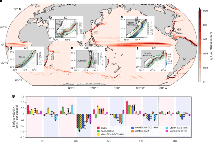
a, Time–mean kinetic energy of surface current in the global ocean based on the ensemble mean of seven high-resolution climate models from 1950 to 2050. b–f, Linear trends of surface velocity (cm s−1 per decade) of five subtropical WBCs: KC (b); GS (c); AC (d); EAC (e); and BC (f). The colour shadings indicate regions that are statistically significant above the 95% confidence level. The solid black lines are the current axes (section ‘The axes of WBCs and onshore/offshore trends’ in Methods). The black arrows indicate the current vectors. The green lines enclose the 1° band on both sides of the axis. g, Magnitude of the velocity trend averaged over the 1° band on the onshore (colour shading) and offshore (line shading) flanks of five WBCs in different models. The black line on each bar represents the error bar based on 1,212 samples for each model and the respective WBC. The grey triangle indicates the trend in each model. The black circles (stars) denote the multimodel ensemble mean on the onshore (offshore) side of WBCs based on seven samples, while the error bars indicate the intermodel spread based on 95% confidence intervals estimated by a bootstrap method. The onshore intensification of WBCs is expected in a warming climate, as indicated by a consensus of all seven available high-resolution climate models.
Source data
Although the impact on upwelling is regionally dependent, enhanced warmings during onshore intensification are observed across all WBCs, contributing to formation of marine heatwaves16. For example, an onshore movement of the EAC, KC and GS is observed to cause an increase in the adjacent shelf temperatures within a range of ~35 km from the EAC core17, a substantial warming of the Pacific Asian marginal seas18 and a fast warming along the US East Coast19,20, respectively. In addition, the warming reduces the solubility of carbon dioxide, which limits the ability of the oceans to absorb anthropogenic carbon dioxide in the atmosphere5,21,22,23 and could destabilize or even lead to a release of a large amount of methane hydrate stored below the sea floor of shelf regions, exacerbating warming of the surrounding climate system24,25.
In response to increasing emissions of GHGs, the WBCs have been found to undergo a poleward intensification26,27,28, featuring an enhanced warming in their extension regions5,29. However, owing to limited ocean current observations and coarse resolution of numerical models, the issue of how the zonal characteristics of the WBCs might change, crucial for projecting changes in marginal seas and coastal areas, remains unknown. Here, using outputs from seven available high-resolution climate models, we find an onshore intensification of global subtropical WBCs under global warming.
Onshore intensification of WBCs
We explore the surface velocity trends of the WBCs over the 1950–2050 period using seven available high-resolution climate models (Supplementary Table 1; section ‘HighResMIP and CESM model simulations’ in Methods). The ocean spatial resolutions of these models are 0.25° or 0.1°, allowing reasonable simulation of the characteristics of a small zonal extent of the WBCs. Six of the seven available models are obtained from the High-Resolution Model Intercomparison Project (HighResMIP)30, run under historical forcing from 1950 to 2014 and shared socioeconomic pathway 585 (SSP 585) forcing from 2015 to 2050. Additionally, a high-resolution simulation based on the Community Earth System Model v.1.3 by the International Laboratory for High‐resolution Earth System Prediction (CESM1.3-iHESP)31 is used, which uses historical forcing from 1950 to 2005 and representative concentration pathway 8.5 (RCP 8.5) forcing from 2006 to 2100. Comparison with observations along typical sections reveals that the models largely reproduce the observed volume transport of WBCs (Supplementary Table 2)32,33,34,35,36,37.
We compute the linear trend of surface velocities in these high-resolution simulations over the period of 1950–2050. The surface velocity trends of five major WBCs (KC, GS, AC, EAC and BC) in the global ocean exhibit zonally opposite trends, with acceleration on the onshore side and deceleration on the offshore side of their axes, respectively (Fig. 1b–f; section ‘The axes of WBCs and onshore/offshore trends’ in Methods). For instance, a positive velocity trend on the western side of the Kuroshio axis extends from the east of Taiwan Island to the Tokala Strait, indicating a greater transport of water near the continental shelf of the East China Sea (Fig. 1b). The deceleration on the offshore side of the GS is more pronounced compared to the acceleration on its onshore side (Fig. 1c), while the AC demonstrates nearly equal rates of acceleration and deceleration (Fig. 1d). Among the five currents, the EAC experiences the strongest onshore acceleration (Fig. 1e), whereas the BC, which is one of the weakest WBCs, exhibits a relatively smaller amplitude (Fig. 1f).
To quantify the onshore acceleration and offshore deceleration of the five WBCs, we calculate the spatial mean velocity trend within a 1° band on both sides of each WBC axis (green lines in Fig. 1b–f). Although the strength of the trends varies among models, the characteristics of a synchronous onshore intensification of all WBCs are robust (Fig. 1g). The onshore acceleration of the KC is represented by a spatial mean amplitude and an intermodel spread, measuring 0.30 ± 0.18 cm s−1 per decade. The most pronounced offshore deceleration among the five WBCs is observed along the GS, reaching −0.94 ± 0.29 cm s−1 per decade. The strength of the mean onshore acceleration and offshore deceleration of the AC is similar. The EAC and BC exhibit the strongest and weakest onshore acceleration among the five currents, with magnitudes of 0.51 ± 0.24 and 0.10 ± 0.08 cm s−1 per decade, respectively (Fig. 1g).
We also use an axis position index (AP) to describe the onshore intensification by comparing the spatial mean trend difference between the onshore and offshore sides of the WBC axis (section ‘Axis position index’ in Methods). The AP suggests a more pronounced acceleration of surface velocities on the onshore flank compared to the offshore flank of all WBCs (Extended Data Fig. 1). The onshore intensification of WBCs is robust in the upper 200 m (Extended Data Fig. 2). The globally synchronous onshore intensification of surface velocity in WBCs suggests that these strong currents bring warm/salty WBC water closer to continental shelves and coastal areas.
We assess the simulated trend in historical simulations (Extended Data Fig. 3a–e). The simulated acceleration trends on the onshore flank of WBCs are smaller than those over the 1950–2050 period. These results are not surprising given that GHG forcing in the historical period is not as strong. The difference between the trend during the historical period and during the entire 1950–2050 period (Extended Data Fig. 3f) ranges from 0.04 ± 0.1 cm s−1 per decade to 0.31 ± 0.18 cm s−1 per decade. In comparison, the onshore acceleration is much larger during the projected (RCP 8.5/SSP 585) simulation period. The projected trend on the onshore flank varies with WBCs, which is 1.5–1.8 times larger than that during 1950–2050. Thus, the change is more pronounced after 2005 as in RCP 8.5 or after 2015 as in SSP 585.
Changes in surface wind and oceanic stratification
The zonal change suggests a globally synchronous acceleration on the onshore flanks of the subtropical WBCs in a warming climate. Potential processes that may lead to the WBC changes include subtropical wind field38,39,40 and oceanic stratification40,41. The subtropical wind field regulates the transport of WBCs and the width of inertial boundary layers, which determines the zonal span and axis position of WBCs. For example, the weakening of the Kuroshio during 1993–2013 resulting from weakened basin-scale wind stress curl is accompanied by more intrusion into the East China Sea42. The oceanic stratification influences the vertical extent of WBCs. Owing to the potential vorticity constraint, WBCs travel along the isobaths over the continental slope in line with their vertical scale40. The enhanced stratification traps the kinetic energy in the upper layer and uplifts the WBCs41 such that WBCs tend to follow shallower isobaths over the slope, leading to a shoreward shifting of their axes. To explore the role of wind and stratification under global warming, we proceed to assess their changes in the climate models.
On the basis of seven climate models, we compute the oceanic stratification and surface wind stress curl in global oceans (Fig. 2). Taking the subtropical North Pacific (SNP) as an example, according to the wind-driven circulation theory, the poleward-flowing KC is driven by the negative wind stress curl over the SNP39,41 (Fig. 2a). Under global warming, the stronger warming at higher latitudes weakens the meridional temperature gradient, leading to weakened westerly winds in the midlatitudes43. Therefore, the negative wind stress curl over the SNP weakens in a warming climate44, manifested as a positive anomaly in the difference of wind stress curl between the historical mean and RCP 8.5/SSP 585 mean (Fig. 2b; section ‘The wind and stratification in each subtropical ocean’ in Methods). Quantitatively, the strength of the spatial mean wind stress curl in the SNP decreases by 3.2% compared to the historical mean.
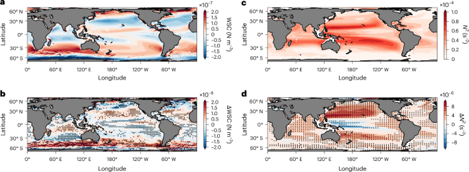
a,b, Time–mean wind stress curls (WSCs) during the historical period (a) and their changes under global warming (b). c,d, Time–mean oceanic stratification averaged at depths between 200 and 400 m during the historical period (c) and changes under global warming (d). All the results are based on the ensemble mean of seven climate models. Changes under global warming are defined as the difference between the mean over the projected period and the mean over the historical period (section ‘HighResMIP and CESM model simulations’ in Methods). The black dots in b and d represent the changes that are statistically significant above the 95% confidence level. In a warming climate, the WSC in global subtropical gyres weakens, but oceanic stratification enhances.
Source data
Compared to the historical average (Fig. 2c), an enhancement in oceanic stratification is evident in the SNP (Fig. 2d). Given that oceanic stratification is primarily influenced by ocean temperature and salinity, we further quantify the respective contributions of these two variables. The spatial mean sea surface temperature (SST, represented by the temperature at the 5 m layer) in the SNP is projected to increase by 1.1 °C under the projected scenario (Extended Data Fig. 4a). The temperature increase is concentrated in the upper ocean and exhibits a decline with increasing depth, resulting in a stronger stratification of the ocean45 (Extended Data Fig. 4k). The SNP experiences a basin-wide freshening due to increased precipitation46 (Extended Data Fig. 4f), but this change in salinity has a secondary impact on oceanic stratification (Extended Data Fig. 4k). The spatial and vertical mean oceanic stratification in the SNP is dominated by temperature changes and is projected to increase by 0.37 × 10⁻⁵ s−2 averaged between 200 and 400 m, indicating a 6.0% intensification compared to the historical mean (6.20 × 10⁻⁵ s−2). A stronger stratification traps more energy in the upper ocean and induces a more surface-intensified circulation system40,47.
Similar to the SNP, the seven-model ensemble mean indicates weakened wind stress curl and intensified oceanic stratification in other subtropical basins under global warming (Fig. 2 and Extended Data Fig. 4), although the westerly in the Southern Ocean intensifies in a warming climate26 (Fig. 2a). In global subtropical gyres, the spatial mean wind stress curl decreases by 0.07–0.46 × 10⁻⁸ N m−3 (1.4–6.4% of the historical mean) and the stratification intensifies by 0.28–0.48 × 10⁻⁵ s−2 (5.3–9.5% of the historical mean) (Supplementary Table 3). Therefore, the relative changes during projected period in stratification are stronger than changes in wind stress curl for most WBCs compared to their historical mean (Supplementary Table 3). The difference in wind and stratification between the first 30 years (1950–1979) and the last 30 years (2021–2050) is consistent with that based on historical and projected means.
Enhanced stratification dominates onshore intensification
To investigate the role of changing oceanic stratification and wind stress curl in affecting the onshore intensification of the WBCs, we examine the relationship between their changes and onshore intensification of the WBCs. For each WBC, we first compute the vertical mean stratification between 200 and 400 m and surface wind stress curl in each subtropical basin (section ‘The wind and stratification in each subtropical ocean’ in Methods). Subsequently, their changes under global warming are calculated on the basis of the spatial mean difference between the historical mean (1950–2005 for CESM-iHESP and 1950–2014 for other models) and the RCP 8.5/SSP 585 mean (2006–2050 for CESM-iHESP and 2015–2050 for other models). The onshore intensification of WBCs displays a strong correlation with enhanced oceanic stratification (based on its averaged value in the subtropical ocean), with a linear correlation coefficient of 0.60, statistically significant above the 99% confidence level (P < 0.01) (Fig. 3a). A stronger oceanic stratification is systematically associated with a greater onshore intensification. In contrast, there is no clear relationship between changes in wind stress curl and the onshore intensification of WBCs (Fig. 3b). Thus, the onshore intensification of WBCs is primarily driven by changes in oceanic stratification.
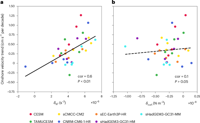
a, Scatterplot of the onshore velocity trends of the WBCs versus changes in oceanic stratification averaged between 200 and 400 m in each subtropical basin under global warming. b, Scatterplot of the onshore velocity trends of the WBCs versus changes in surface wind stress curl averaged in each subtropical basin under global warming. Changes in oceanic stratification and wind stress curl are calculated as the difference between the historical mean and the projected mean (section ‘The wind and stratification in each subtropical ocean’ in Methods). The solid line in a represents the linear regression with a statistically significant correlation coefficient (cor) of 0.60 (P = 2 × 10⁻⁴, two-sided test), while the fit in b indicates a non-significant correlation coefficient of 0.10 (P = 0.57, two-sided test). In each model, the onshore velocity, the changes in stratification and the changes in wind stress curl are scaled by the global mean SST difference between the projected mean and the historical mean. Under greenhouse warming, the WBC onshore intensification is more associated with increased oceanic stratification than with weakened wind stress curl.
Source data
To confirm the relative importance of changing wind and stratification in affecting the zonal structure of the WBCs, we conduct a set of idealized high-resolution experiments based on the Massachusetts Institute of Technology general circulation model48 (MITgcm) (section ‘MITgcm model’ in Methods). The model domain consists of a shallow coastal shelf and a flat deep ocean connected by a continental slope (Extended Data Fig. 5a). Since the intensified stratification in the subtropical gyres is primarily determined by temperature variations, the ocean salinity is maintained constant at 35 g kg−1, while the vertical temperature profile is averaged over each subtropical basin (Extended Data Fig. 5b). Hence, the stratification follows the changes in temperature. The wind forcing is represented by an idealized cosine zonal wind stress, with easterly trade winds in low latitudes and westerly winds in midlatitudes (Extended Data Fig. 5c).
For each WBC, the associated experiments consist of a simulation forced with climatological mean wind forcing and oceanic temperature field obtained from observations and reanalysis data (CTRL run), a simulation with warming-induced changes in both wind forcing and stratification (WARMING run) and two simulations considering changes in stratification (ΔN2 run; N2 indicates buoyancy frequency) and wind forcing (ΔWIND run), respectively. In the last three runs, the changes in stratification and wind forcing are based on the difference between the historical period and projected warming scenarios in the seven climate models. As such, comparisons between these simulations allow us to assess the behaviour of WBC axes in a warming climate and the relative importance of changes in stratification and wind forcing.
We use the SNP as an example to describe the dynamics (Fig. 4a–d). Processes in other basins are similar (Extended Data Fig. 6 and Supplementary Table 4). In the CTRL run (Fig. 4a), the Kuroshio flows along the continental slope with a maximum around 1.0 m s−1, in accord with in situ observations1. In a warming climate (Fig. 4b), the poleward velocity anomalies exhibit a dipole pattern with acceleration on the onshore flank and deceleration on the offshore flank of the mean current axis, consistent with climate models. Given that the ocean becomes shallow on the onshore flank, a shallower Kuroshio is seen under global warming. In the ΔN2 run, enhanced stratification results in a similar dipole pattern along the Kuroshio axis (Fig. 4c), suggesting that the onshore intensified Kuroshio is mainly induced by enhanced stratification. By comparison, notable deceleration is found on the offshore flank in the ΔWIND run (Fig. 4d), indicating that weakened wind primarily leads to an overall weakening rather than an onshore intensification of the Kuroshio. Furthermore, the evolution of the Kuroshio can also be revealed by comparing the normalized transport distribution in the four runs. The increased (decreased) transport on the onshore (offshore) flank in response to global warming reflects an onshore intensification of the Kuroshio.
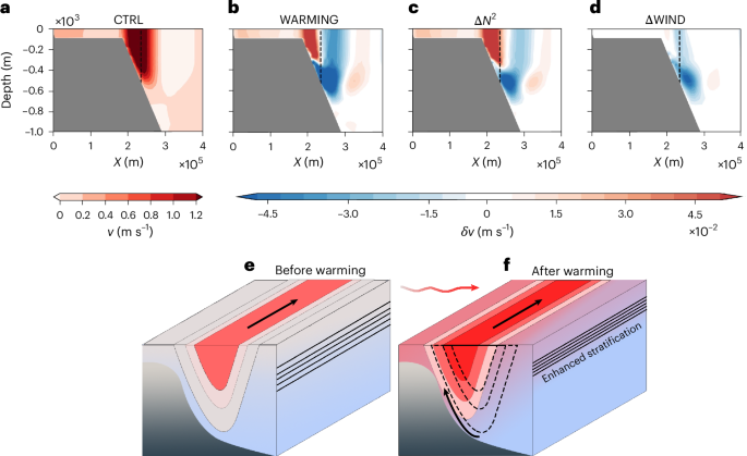
a, Vertical section of the meridional velocities in the western boundary region of the CTRL run. b–d, Meridional velocity changes in WARMING run (b), ∆N2 run (c) and ∆WIND run (d) relative to the CTRL run. The dashed line denotes the axis of the Kuroshio. The vertical section is located at the meridional centre of the model domain (Extended Data Fig. 5a). e, Schematic showing the vertical structure of the WBC before warming, during which the ocean is weakly stratified and the vertical extent of the WBC is large. f, Schematic showing the vertical structure of the WBC after warming when the ocean stratification is enhanced, leading to a vertical shrinking and shoreward movement of WBC (curved arrow; compare solid and dashed lines). The colour shadings denote the ocean temperature and the solid black lines indicate the isotherms. The onshore intensification of WBCs is dominated by a warming-induced intensification in oceanic stratification.
Source data
To compare the roles of wind and stratification quantitatively, we introduce two indices. An AP describes the contribution of onshore flank transport relative to that in the CTRL run (section ‘Axis position index’ in Methods). By definition, AP in the CTRL run is 0. In addition to the change of the axis position, the onshore intensification of a WBC is accompanied by its shallower structure. Therefore, a WBC depth index (D) is defined (section ‘Vertical scale of WBCs’ in Methods)49,50 as
and is taken as a proxy of the onshore intensification. In equation (1), |curl(τ)| and N2 describe the roles of wind stress curl and oceanic stratification, respectively. By substituting the wind stress curl and temperature profile from the CTRL run into equation (1), we obtain the reference value of D (292.1 m). Enhanced stratification and weakened wind field could lead to a smaller D.
Under global warming, a 6% increase in oceanic stratification (0.37 × 10⁻⁵ s−2) and a 3% decrease in the wind stress curl over the SNP (0.23 × 10⁻⁸ N m−3), as projected by the seven climate models, lead to changes in the AP and D of 1.35 × 10⁻² and −9.4 m, respectively. By separately considering the independent effect of stratification and wind, we find that the enhanced stratification dominates changes in AP and D (0.95 × 10⁻² and −6.5 m), whereas the weakened wind stress curl has a minor impact, with changes in AP and D of 0.46 × 10⁻² and −3.0 m, respectively. To further investigate the role of oceanic stratification in other WBCs, we conduct a series of experiments similar to the SNP (section ‘MITgcm model’ in Methods). The onshore intensification, reproduced for all WBCs, is primarily driven by changes in oceanic stratification (Extended Data Fig. 6 and Supplementary Table 4).
To test the robustness of the associated dynamics, we also conduct a series of experiments with realistic temperature, salinity, wind forcing and bottom topography (section ‘MITgcm model’ in Methods). The simulations reproduce the acceleration on the onshore flank (Supplementary Fig. 1), which is mainly induced by the enhanced stratification (Supplementary Fig. 2), consistent with our idealized model. Thus, global warming intensifies oceanic stratification, causing the current to be compressed into a shallower layer and to travel along shallower isobaths over the continental slope. As a result, the WBCs shift to shoreward regions (Fig. 4e,f).
Summary and implications
Our finding of an onshore intensification of global subtropical WBCs under greenhouse warming is underpinned by an intensified ocean stratification. This onshore intensification is also seen in observations, although with varying uncertainties among different WBCs due to a short observation period7,20,51. The intensified stratification is in turn driven by a faster warming near the surface ocean than the ocean below, which is robust across models, including the high-resolution models that reasonably resolve the swift narrow structure of WBCs. Our finding of a WBC onshore intensification could have profound implications. A reduced upwelling in the Agulhas Bank and the Southeast Brazilian Bight probably induces low-nutrient conditions, as seen when an anomalous reduction in upwelling occurs12,13,15 that could disrupt the ecological balance of the regions. Further, as a consequence of the enhanced warming from the onshore intensification, more intense marine heatwaves52, a reduced ocean ability to absorb carbon dioxide5,21,22 and an increased risk of destabilized methane hydrate below the shelf sea floor24,25, are likely to occur. Thus, our result highlights the needs for a comprehensive assessment of the associated impacts.
Methods
HighResMIP and CESM model simulations
To investigate the projected long-term trends of the velocity on the two sides of the WBCs in future climate, we use seven climate models. Six of these seven models (14 experiments) are obtained from the HighResMIP30 (Supplementary Table 1) of the coupled model intercomparison project phase 6 (CMIP6)53. To assess benefits of increased horizontal model resolution, ‘standard’ HR models in HighResMIP are configured with an ocean grid spacing of 0.25° or 0.1° (Supplementary Table 1) together with a range of atmosphere resolutions. A spin-up of 30–50 years is made for each model using constant 1950s forcing. After spin-up, all models are run under time-varying historical forcing from 1950 to 2014 (hist-1950 run) and future GHG forcing following the SSP 585 emission scenario for the period 2015–2050 (high-resolution future run). This scenario incorporates an extra radiative forcing of 8.5 W m−1 (ref. 53) by the year 2100. In this study, monthly outputs (that is, horizontal velocity, potential temperature and wind stress) from the six HighResMIP models are used. To avoid dominance by models in which multiple experiments are preformed, the experiments of EC-Earth-3P-HR (ref. 54), CMCC-CM2 (ref. 55), HadGEM3-GC31-HM and HadGEM3-GC31-MM (refs. 56,57) are averaged first in each model before calculating the multimodel statistics. The period used in this study is from 1950 to 2050.
In addition to HighResMIP products, model outputs from the monthly CESM1.3-iHESP from 1950 to 2050 are also used31. The model contains the Community Atmosphere Model v.5 (CAM5) as its atmosphere component and the Parallel Ocean Program v.2 (POP2) as its ocean component. The resolutions of CAM5 and POP2 are 0.25° and 0.1°, respectively. The ocean component of the CESM1.3-iHESP is initialized with a rest ocean and the mean January climatological potential temperature and salinity from the World Ocean Atlas, while atmosphere component is spun up from restart files of previously performed simulations. The simulation consists of a 500 year pre-industrial control simulation (PI-CTRL) run, a 250 year historical (1850–2005) and a future RCP 8.5 (2006–2100) transient climate simulation (HF‐TNST) run from 1850 to 2100 branched from PI‐CTRL at year 250. It should be noted that CESM1.3-iHESP is forced under the CMIP5 experimental protocol and therefore is different from the CESM model participating in HighResMIP, which is otherwise provided by Texas A&M University (TAMU) and for differentiation is designated as CESM-TAMU in this study.
It should be noted that the time periods in the CMIP6 models slightly differ from those in the CESM1.3-iHESP model. Therefore, the historical period refers to 1950–2014 for the CMIP6 models and 1950–2005 for the CESM1.3-iHESP model, while the projected period refers to 2015–2050 for the CMIP6 models and 2006–2050 for the CESM1.3-iHESP model, respectively. Despite this difference, both the SSP 585 and RCP 8.5 scenarios effectively represent the climate system subject to greenhouse warming.
In this study, the significant confidence levels of time-related linear trends are estimated using 95% Student’s t-test confidence level. The significant confidence levels associated with intermodel uncertainty are estimated using 95% bootstrap confidence intervals. The bootstrap confidence intervals are computed from 2,000 samples.
The axes of WBCs and onshore/offshore trends
The axis of a WBC is defined by the location of maximum along-stream velocity based on the historical mean. Here, the historical period is 1950 to 2014 for the HighResMIP products and from 1950 to 2005 for the CESM1.3-iHESP model, respectively. The spatial mean trend of surface velocity on both sides of the axis is calculated by averaging within a 1° band on the western and eastern sides of the axis (green lines in Fig. 1b–f). Furthermore, since the current velocity in the ocean interior is generally weaker compared to that in WBCs, we have omitted the trend where the mean velocity is <0.15 m s−1 in Fig. 1b–f, to emphasize the trend along the WBCs. To focus on the long-term trend, we apply a 10 year low-pass filter to the yearly mean data before calculating the trend. Linear trends of surface velocity in five subtropical WBCs are calculated from 1950 to 2050 using the least-squares method and tested against the 95% confidence level using a Student’s t-test.
Axis position index
AP is used to describe the onshore intensification of the WBCs in both the climate model and the idealized MITgcm simulations. In the climate model, AP is defined as the difference between the spatial mean trend of surface velocity on the two sides of the axis (onshore minus offshore). A larger AP indicates a stronger onshore acceleration in surface velocity on the onshore side compared to the offshore side. In the idealized MITgcm simulations, we first get the axis of WBC in CTRL run based on the velocity field. Next, we calculate the transport on the onshore (offshore) flanks of the WBC in each run based on the axis of WBC in CTRL. Then, the onshore (offshore) flank transport is scaled by the total transport of the WBC in each run. Next, we calculate the transport difference on the two flanks of the axis (onshore minus offshore). Finally, the AP in each run is defined as the anomaly of this transport difference relative to that in the CTRL run. Therefore, the AP value is 0 in the CTRL run, while a positive AP indicates an onshore intensification of WBCs.
The wind and stratification in each subtropical ocean
Wind stress curl and oceanic stratification are calculated on the basis of an ensemble mean of the seven climate models. Time–mean wind stress curl is calculated during the historical period, while the changes are defined as the differences between the historical period (1950–2005 for CESM-iHESP and 1950–2014 for other models) and the projected period (2006–2050 for CESM-iHESP and 2015–2050 for other models). The extent of each subtropical gyre is defined as follows: the SNP Ocean (15° N–30° N, 120° E–90° W), the subtropical North Atlantic Ocean (20° N–35° N, 90° W–0°), the subtropical South Indian Ocean (35° S–20° S, 20° E–120° E), the subtropical South Pacific Ocean (35° S–20° S, 145° E–75° W) and the subtropical South Atlantic Ocean (35° S–20° S, 70° W–0°) (Extended Data Fig. 7).
We use the Brunt–Väisälä frequency (N2) to describe the oceanic stratification, which is calculated through the Gibbs Seawater Oceanographic Toolbox v.3.05 based on the international thermodynamic equation of seawater-2010, using temperature and salinity data from the ensemble mean of the seven climate models58. To quantify the relative contribution of temperature and salinity changes to the overall variation in stratification, we first calculate the stratification during the historical period. Then we consider the changes in temperature and salinity separately, obtaining temperature-induced stratification changes (red line in Extended Data Fig. 4k–o) and salinity-induced stratification changes (blue line in Extended Data Fig. 4k–o), respectively, under global warming59,60. By considering both temperature and salinity changes, we calculate the total changes of stratification owing to global warming (black line in Extended Data Fig. 4k–o).
MITgcm model
To investigate the mechanism of the WBC onshore intensification in a warming climate, the MITgcm48 is used. The model solves the primitive equations of motion on a staggered C grid in the horizontal and depth coordinates in the vertical. The model domain is a rectangle with closed lateral boundary conditions. The meridional extents of the domains are 1,500 km, while the zonal extents range from 5,000 to 10,000 km for different subtropical gyres. Zonal extents in idealized runs are 10,000 km (the North Pacific Ocean), 8,000 km (the North Atlantic Ocean), 8,000 km (the South Indian Ocean), 10,000 km (the South Pacific Ocean) and 5,000 km (the South Atlantic Ocean). The model domain consists of a 200-km-width shelf (with a depth of 100 m) near the western boundary, followed by a 100-km-wide continental slope extending from 0 to 1,000 m. The slope further extends to the deep ocean floor (2,000 m in depth; Extended Data Fig. 5a). The meridional resolution is 10 km, whereas the zonal resolution is 10 km from the western boundary (0 km) to 1,500 km (covering the continental shelf and slope regions) and 25 km from 1,500 km to the eastern boundary. Vertically, the model is configured using 45 levels with 10 m intervals in the upper 200 m, increasing to 200 m at the bottom. The model uses a beta plane approximation. The Coriolis parameters at the southern limit of the domains are 3 × 10⁻⁵ s−1 for the northern hemisphere and −6.12 × 10⁻⁵ s−1 for the southern hemisphere, with meridional variation β = 2 × 10⁻¹¹ m−1 s−1. Horizontal and vertical viscosity coefficients are 200 and 10−4 m2 s−1, respectively. Vertical diffusion coefficient is 10−5 m2 s−1.
Four runs are conducted for each WBC, including a CTRL run representing the historical state and three runs (WARMING run, ΔN2 run and ΔWIND run) representing changes in a warming climate. In the CTRL run, temperature profile, salinity profile (for the salinity diagnostic runs) and wind forcing are obtained from the World Ocean Atlas 2018 (WOA18)61,62 and the European Centre for Medium-Range Weather Forecasts Reanalysis v.5 (ERA5)63 during 1950–2000. The temperature profile is horizontally averaged over each basin (Extended Data Fig. 5b). Then, the stratification is vertically averaged over the depth of 200–400 m based on the temperature profile (Supplementary Table 3). The wind forcing is set to be an idealized cosine-like zonal wind stress, with an easterly trade wind in low latitudes and a westerly wind in midlatitudes (Extended Data Fig. 5c), where the amplitude is based on ERA5 and averaged in each subtropical ocean. In the WARMING, ΔN2 and ΔWIND runs, the anomalies in SST and wind stress are based on the difference between the historical simulations and the projected simulation of the ensemble mean of the seven climate models. The anomaly of temperature profiles is simplified as a downward exponential function decaying from the sea surface to the bottom, with an e-folding scale of 200 m, where the changes in stratification are consistent with the prediction of the climate model. Detailed model parameters for all basins are summarized in Supplementary Table 3.
In addition to the idealized model, we also conduct a series of more realistic experiments. These new simulations use wind forcing and temperature/salinity (T/S) anomalies derived from the ensemble mean of climate models. For each WBC, we conduct two runs: one uses historical mean T/S, wind and data based on the WOA18 and the ERA5; the other uses anomalies corresponding to the difference between the RCP 8.5/SSP 585 scenario and the historical scenario based on climate models. The horizontal resolution is 0.25°. Vertically, the model is configured with 48 levels, with 10 m intervals from the top layer to 387 m, totalling 5,000 m. The topography is sourced from the WOA18. The model extent for each WBC is defined as follows: the KC (10° N–40° N, 105° E–99° W), the GS (0.5° N–42.5° N, 104° W–5° W), the AC (51° S–9° S, 11° E–119° E), the EAC (51° S–0°, 137° E–70° W) and the BC (51° S–0°, 67° W–20° E). The model domain for each WBC is set to cover the entire subtropical basin for simulating each WBC. To focus on the changes associated with wind and stratification in the subtropical ocean, a zero-velocity boundary is applied. Additionally, to preserve the basin-scale temperature and salinity patterns, boundary T/S data are used. All models are run for 50 years, with the time–mean of the last 10 years used for analysis. The other configurations remain consistent with those detailed in the idealized model.
Vertical scale of WBCs
The vertical scale of a wind-driven WBC is estimated by a vorticity balance. For the interior flow, the Sverdrup balance is
where Vs is the meridional mass transport over unit zonal distance, f is the Coriolis parameter, β is the meridional variation of the Coriolis parameter, τ is the wind stress and k is the vertical unit vector. This equation illustrates that the meridional mass transport (Vs) is determined by wind stress curl (curl(τ/f)), f and β. For the WBC over a topographic slope, the change in planetary vorticity is mainly balanced by stretching64,
where y is meridional distance, N is buoyancy frequency, ψ is streamfunction and ψzz indicates its vertical second derivative. To simplify these equations, the variables in equations (1) and (2) could be non-dimensionalized using the following scaling:
where * denotes the non-dimensional quantity, U represents amplitude of the horizontal velocity, L is meridional length scale, D is vertical length scale and ({rho }_{0}) is seawater density. Thus, solving non-dimensional equations (1) and (2) allows for derivation of the vertical length scale (equation (1)). Therefore, the vertical scale of a wind-driven WBC is directly proportional to the Coriolis parameter (f) and wind stress curl (({rm{curl}}left({mathbf{uptau}}right))), while it is inversely proportional to stratification (N2), meridional variation of the Coriolis parameter (β) and seawater density (({rho }_{0})). This method has been used in previous studies to explain the vertical scale of wind-driven circulation near continental or island boundaries49,50.
Reporting summary
Further information on research design is available in the Nature Portfolio Reporting Summary linked to this article.

Responses