Winter subglacial meltwater detected in a Greenland fjord
Main
In Greenland, marine-terminating glaciers release meltwater at depth, causing a mixing of buoyant meltwater and saline ocean water1,2. The discharge of subglacial meltwater and subsequent mixing leads to an upwelling of deep fjord waters close to the glacier fronts, influencing the circulation in the fjord systems3,4. The meltwater impacts glacial frontal melt5,6 and ice mélange melt7, thereby modifying the mass loss from marine-terminating glaciers and consequently glacier contribution to future sea-level rise8,9. The upwelling also impacts the influx and mixing of nutrients10,11,12, enhancing biological primary productivity and providing feeding grounds for fish and seabirds13,14.
Greenland fjords experience large seasonal variability in temperature and salinity4,15. During the summer, subglacial meltwater, predominantly from surface runoff, has been observed in fjord waters as a layered structure below the surface layer7. In contrast, winter measurements of subglacial discharge into Greenland fjords are effectively unprecedented. Thus, the volume of winter subglacial discharge and its impact on fjord systems remains an open question16, and model estimates of winter meltwater differ by orders of magnitude5,17,18. Measurements in Kangersuneq (in Nuup Kangerlua, west Greenland) revealed a considerable difference in temperature–salinity profiles between summer and winter, suggesting no noteworthy freshwater outflow from nearby glaciers during winter1. Studies of the Milne Fjord epishelf lake, northern Canada, report similar findings suggesting that winter freshwater discharge is negligible19. In contrast, studies from Svalbard fjords have found evidence of freshwater input during winter20,21 and early spring22. However, owing to the shallow fjord depths (tens of metres), and consequently shallow grounding lines21,22, this meltwater is probably added directly into the fjord surface layers, implying that its effect on fjord circulation is separate from subglacial freshwater discharged at depth (hundreds of metres).
In contrast to observations, theoretical estimates of winter freshwater volumes indicate that subglacial meltwater discharges at depth into Greenland fjords all year round17,18,23. However, fjord circulation models disagree on the importance of winter discharge for heat and water exchange24,25. In the absence of other freshwater fluxes, the winter discharge of glacial meltwater may have a pronounced influence on fjord dynamics, but its impact will depend on water volumes and fjord/glacier settings16. This underscores the complexity of bathymetry and heat exchange dynamics between the shelf and marine-terminating glaciers within individual fjords. Finally, the fast-changing Arctic climate may already be causing shifts in wintertime conditions, highlighting the urgency for a better understanding of wintertime dynamics. To our knowledge, our study is the first to measure and document the existence of subglacial freshwater in a Greenland fjord during winter, shedding light on a hitherto undocumented process.
In situ observations of temperature and salinity
During a dedicated field season in March 2023, we carried out in situ observations of water properties at Eqalorutsit Kangilliit Sermiat (at times referred to as Qajuutaap) and neighbouring fjords (Fig. 1). Eqalorutsit Kangilliit Sermiat is one of the largest marine-terminating glaciers in south Greenland (its drainage basin and discharge rates are matched only by neighbouring Eqalorutsit Killiit Sermiat23,26) with an ice front grounded several hundred metres below sea level and a grounding line depth that in places exceeds 400 m below sea level27. The glacier discharges into an eastern branch of Sermilik Fjord, which forms the inner part of Ikersuaq Fjord (formerly Bredefjord). The fjord depth ranges from 60 to 600 m below sea level, but bathymetric maps in the middle part of the fjord are highly uncertain due to a lack of in situ observations.

The locations of our measurement stations are indicated with coloured circles, with measurements acquired by our UAV outlined with a thick black line. Measurements from the OMG project30 and the GINR (KR23034) are indicated with a brown diamond and brown triangle, respectively. PROMICE AWS are marked with black stars. Ice-marginal lakes are outlined with turquoise44, and the ice sheet is coloured grey with 200-m surface topography contours in thin grey lines from refs. 27,57. The background image is optical satellite data from Sentinel-2 (Copernicus Sentinel data, processed by the European Space Agency) from 27 March 2023. The location of the map is indicated on the overview map in red, also showing 500-m surface topography contours27,57 and surface velocities in blue58.
To retrieve temperature and salinity measurements, we developed and deployed a novel uncrewed aerial vehicle (UAV) solution (Fig. 2). Dense ice mélange has prevented previous studies from acquiring measurements in glacial fjords during winter, and the UAV was crucial to our success. The UAV platform consists of a modified kit helicopter with an onboard autonomous winch and a commercial conductivity, temperature and depth (CTD) sensor payload (see ref. 28 and Methods). Its maximum total flight time is 24 min, allowing for measurements to be collected up to a distance of 6 km, although our measurements were acquired less than 1.5 km from the deployment sites. We carried out additional CTD deployments in front of Eqalorutsit Kangilliit Sermiat, where flat, walkable fjord ice enabled us to drill two holes manually in the ice (Fig. 3). The heavy fjord-ice conditions in neighbouring Tunulliarfik Fjord also made it possible to drill a hole manually and make CTD casts.

a, Complete UAV platform with CTD payload extended. b, UAV during profiling in a narrow section of open water created by a seal. The seal hole in the sea ice is smaller (approximately 0.5 m) than the flooded surface area. Note the line extending from the UAV to the submerged CTD instrument. The UAV platform has a length of 1.145 m and a rotor diameter of 1.455 m. Photos are from two different deployments.
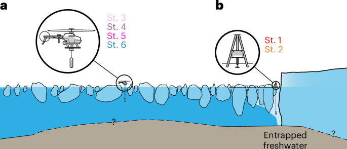
Side-looking schematic view of our measurement site. Dashed lines indicate that fjord bathymetry and glacier bed topography are poorly constrained. Light blue colours in the water indicate entrapped freshwater. a, b, Enlarged versions of our measurement techniques. The measurements in the ice mélange (St. 3–6) (a) were retrieved using our UAV platform, while the measurements by the glacier front (St. 1 and 2) (b) were conducted by drilling through the ice and manually deploying a CTD cast.
Temperature and salinity data were derived from the CTD profiles, and salinity was calculated using the Practical Salinity Scale 1978. In the upper 30 m, temperature and salinity conditions cluster in three characteristic patterns (Fig. 4): the coldest and freshest conditions were found near the glacier front (Station (St.) 1 and 2; orange and red lines, respectively), transitioning to slightly warmer and saltier water in the ice mélange (St. 3, 4, 5 and 6; rose, magenta, pink and blue lines, respectively) and Sermilik Fjord (St. 7; turquoise lines). Compared with these measurements, conditions in Tunulliarfik Fjord (St. 8, yellow line) are warmer and saltier, indicating that coastal water modifies the fjord waters. Below 40 m depth, measurements closest to the glacier front (St. 1 and 2) reach salinity levels similar to those in Tunulliarfik Fjord (St. 8). For context, we include summer measurements from the Oceans Melting Greenland (OMG) project29,30 and from the Greenland Institute of Natural Resources (GINR; Fig. 4, brown lines).

a–c, CTD profiles of temperature (a) and salinity (b), and the corresponding T–S diagram (c; locations are shown in Fig. 1). Observations from the GINR (KR23034, June 2023) and the OMG project (August 2018) are shown as brown lines. Dotted lines indicate measurements from neighbouring Tunulliarfik Fjord. A GINR winter observation from Nuup Kangerlua in west Greenland is shown in black (GF10099, April 2010). A Gade slope of 2.5 °C per salinity unit is indicated with thick grey shading. The freezing point line of seawater is shown as a dashed–dotted grey line. Arrows indicate the two-temperature minima seen in St. 1 and 2 data.
Source data
In the temperature–salinity (T–S) diagram (Fig. 4c), St. 1 and 2 measurements show a two-minima temperature profile (black arrows). Previous studies have interpreted two-minima temperature profiles as subglacial discharge1,7. In contrast, two-minima temperature profiles are not seen in our CTD observations from the ice mélange (St. 3–6) or Sermilik Fjord (St. 7). The down-fjord observations (St. 3–6) display a halocline layer (15–38 m depth) in the T–S diagram that follows a melt line with an observed slope of 2.5 °C per salinity unit, which corresponds to the Gade slope31. According to the Gade model31, the mixing of melted glacial ice with seawater appears as a straight line in a T–S diagram with a slope of about 2.5 °C per salinity unit. Thus, the down-fjord observations indicate that the freshening can be explained solely by the melting of ice mélange and stranded icebergs, while the freshening observed at St. 1 and 2 is caused by a mix of melt from ice mélange and icebergs, and subglacial discharge. Notably, measurements from St. 1 and 2 follow the same T–S line as water in Tunulliarfik Fjord (St. 8), indicating an influence from coastal water.
Figure 4 also includes a rare winter observation from Nuup Kangerlua in west Greenland acquired ~4 km from the glacier front of Kangiata Nunaata Sermia (black line, referred to as GF100991). A halocline layer (below 17 m depth) caused by melting of the ice mélange can be seen in our down-fjord observations (St. 3–8) and in GF10099. Comparison with our St. 1 and 2 measurements highlights the novelty of our observations. Where the surface layer temperature of GF10099 follows the freezing line, St. 1 and 2 profiles do not reach the freezing point and have local temperature minima, showing a likely input of warmer waters such as a mixture of ambient deep fjord waters and subglacial meltwater discharge. Based on our observations, we suggest that (1) meltwater enters the fjord subglacially from Eqalorutsit Kangilliit Sermiat, freshening the surface layer; and (2) the meltwater accumulates at the glacier front under the mélange in a ‘fresh surface pool of water’ (Fig. 3) similar to reported epishelf lakes19.
Freshwater volumes and sources
To our knowledge, our study is the first to document the existence of subglacial meltwater in a Greenland fjord during winter and to report evidence of upwelling at depth. The two-minima signal in our data is not as strong as observed during summer conditions (Fig. 4, brown lines; also ref. 4), indicating that the subglacial discharge may not be substantial. The fact that the freshwater pool is spatially confined is the likely reason why it has not been observed by previous studies, as measurements in those studies were retrieved 4 km (ref. 1) and 6 km (ref. 32) from the glacier front compared with our measurements, which were 1 km (St. 1), 1.7 km (St. 2) and 5 km (St. 3) from the front.
Subglacial water may have different provenances. During summer, subglacially discharged water derives predominantly from surface meltwater that enters the subglacial system via moulins and crevasses33. During winter, in the absence of surface melt, the origin of the water is less clear. We suggest that the observed pool of meltwater originates from basal melting, that is, from melting at the interface between ice and bedrock. The basal conditions of the Greenland ice sheet are not well known, but estimates indicate that large parts of the ice sheet’s base are at the melting point34. Studies suggest that basal melt is predominantly caused by heat from friction and geothermal flux17,35, and therefore, basal melt discharges during all seasons, making basal meltwater a potential source of wintertime freshwater.
Other potential freshwater sources include surface melt and glacier-lake drainage events. Here we outline why we discard these two meltwater sources as explanations for our measurements. Firstly, while large volumes of surface meltwater enter Sermilik Fjord in the summertime, the winter surface melt volume is orders of magnitude smaller due to low air temperatures (Extended Data Fig. 1). We estimate the likely surface melt using an improved Positive Degree Day (PDD) model36 and in situ measurements from the Programme for Monitoring of the Greenland Ice Sheet (PROMICE) Automatic Weather Stations (AWS37; Fig. 1 and Methods). Our results indicate that surface melt occurred for two days in early March (Extended Data Fig. 2). Only the lowest-elevation AWS experienced surface melt with daily melt rates of 5.6 mm and 6.4 mm on 2 and 3 March, respectively (three weeks before our measurements began). Given the small volume of meltwater generated, we posit that the water is unlikely to have penetrated to the bed of the glacier and that the majority of the water was retained and refrozen close to the ice surface, either in the broken and weathered bare-ice surface or in snow pockets38. This is supported by observational evidence of refrozen ice, snow pockets and dry crevasses at the glacier margin (Extended Data Fig. 3).
While we discard recent surface melt as a potential source of freshwater, a delayed release of surface meltwater generated during the previous melt season could contribute to the observed freshwater signal. The travel time of meltwater in the Greenland subglacial system is poorly constrained; however, numerous studies (as summarized in ref. 39) have found evidence that the subglacial system drains highly efficiently, indicating an overall limited storage capacity. This is supported by a recent study that used measurements of shifts in the Greenland bedrock to estimate that the water storage time in south Greenland is on average 31 days with an uncertainty of 12 days (ref. 40). Local topography may further promote surface water storage by pooling water into subglacial lakes. For example, evidence of winter meltwater from a land-terminating glacier in Greenland41 was found upstream of an area previously identified as a potential area for subglacial water storage42. However, no subglacial lakes have been identified in our study area43. Lacking isotope measurements, we cannot disentangle surface meltwater from basal meltwater and it is possible that our observations represent a mix of both meltwater sources.
A second freshwater source is the drainage of ice-marginal lakes. Thus, we investigated 21 lakes that share a margin with the glacier’s catchment area (mapped in 201744). Between January and April 2023, 5 of the 21 ice-marginal lakes around the lateral margins of Eqalorutsit Kangilliit Sermiat could be identified. Little is known about the dynamics of these lakes; however, satellite images suggest that their areas varied insubstantially during our period of interest and there is no evidence of glacial lake outburst floods or full drainage events during this period (Methods and Extended Data Fig. 4).
Other sources of freshwater at glacier fronts include melting of the glacier front itself. The frontal melt contribution to the freshwater budget of fjords is unresolved and recent laboratory studies suggest that frontal melt may be underestimated in models45. Nevertheless, observations in a Greenland fjord showed that the contribution from frontal melt is minor due to the small front surface compared with the ice mélange surface7. Importantly, meltwater originating from frontal melt will follow the Gade slope; therefore, if the freshwater signal consisted of only frontal meltwater, we would not observe a two-minima temperature profile.
To our knowledge, our study is the first to successfully measure meltwater linked to basal meltwater at a glacier front as opposed to precipitation or surface melt20,41. The estimated monthly basal melt of Eqalorutsit Kangilliit Sermiat is 3.8 × 10⁶ m3, corresponding to 2% of the glacier’s annual mass loss23. This estimate is highly uncertain, and we leverage our CTD observations to evaluate the amount of freshwater necessary to cause the observed freshening. Our results indicate a freshwater volume corresponding to 2.4 × 10⁵ m3 (Methods and Extended Data Fig. 5). This estimate includes all sources that contribute to freshening the water at the front, including meltwater from the glacier front and the delayed release of surface meltwater, and it should, therefore, be considered an upper bound. Nevertheless, our estimate is an order of magnitude lower than the theoretically estimated monthly basal melt. We suggest several reasons for this discrepancy that are not mutually exclusive. Firstly, the source area for the basal meltwater is reconstructed based on surface and bed topography, where the latter has uncertainties upwards of 300 m (ref. 27). Therefore, the source area may be smaller than estimated, lowering the modelled basal meltwater volume discharging at the glacier front. Secondly, studies suggest that the subglacial system can shut down during winter46, blocking the transport of basal meltwater from upstream parts of the glacier basin. This potential disconnection between parts of the subglacial system may be highly dependent on ice-flow velocities and the glacier’s topographic setting. Finally, our St. 1 and 2 measurements were acquired in a small bay a few kilometres east of where the glacier plume emerges in the summer. If it had been possible to get closer to the plume’s likely central outflow, we might have seen a stronger freshwater signal.
Impacts of winter meltwater discharge
Our measurements indicate that basal meltwater released subglacially during winter modifies near-glacier water properties and influences processes controlling ice/fjord interactions, fjord dynamics and ecosystems. Modelling studies of summer plumes47 have shown that upwelling of Atlantic water driven by plumes may substantially warm near-glacier waters at intermediate depth, affecting the distribution and magnitude of frontal melt. We suggest that winter discharge will have a similar effect, that is, enhanced mixing and entrainment of ambient water at the glacial front. Ambient water temperatures above 0 °C, typically from Atlantic water, will accelerate frontal melting. Conversely, for glaciers terminating in water with ambient temperatures below 0 °C, winter discharge may promote refreezing and frazil ice formation in the fjord48. Thus, glaciers in contact with warmer waters, such as those in southwest Greenland49, are especially vulnerable to the effects of winter discharge, and an increase in winter freshwater would lead to increased frontal melt. However, there is a lack of understanding regarding the seasonal variation of water mass properties near glaciers and subglacial discharge outside the summer months16, and more work is needed to include this effect in projections of future glacier mass loss from oceanic forcing, for example, ref. 9. Thus, our findings underscore the urgent need to understand the role and impact of winter subglacial discharge on fjord dynamics.
The winter subglacial discharge from Eqalorutsit Kangilliit Sermiat probably replenishes nutrients in the surface waters, thereby readying the system for expansive primary production during spring when the ice mélange breaks up. Hence, winter subglacial discharge in the inner parts of fjords may play a more critical role in priming the spring phytoplankton production than previously anticipated. It has been reported that the spring bloom in a marine-terminating glacier fjord will be triggered by out-fjord winds and coastal inflows driving an upwelling in the inner part of the fjord, hereby supplying nutrient-rich water to the surface layer50. Our observations suggest that winter subglacial discharge may entrain nutrients from deeper waters and accumulate them in a surface pool of water beneath the ice mélange near the glacier front. As a result, favourable conditions for a spring phytoplankton bloom are expected to establish when the mélange breaks up, as observed further north in the Nuup Kangerlua fjord system51. It is noteworthy that the spring bloom might not occur directly in front of the glacier but further out in the fjord, as the nutrient pool will track the drifting ice pushed by prevailing winds from the northeast during spring (see observed wind directions in Extended Data Fig. 6). This further underscores the seasonal significance of marine-terminating glaciers in stimulating primary production.
Observations and models suggest that subglacial discharge causes fjord circulation patterns that lead to a renewal of fjord basin waters over seasonal time scales2,52. Although melt from icebergs and ice mélange probably dominates the winter freshwater budget for most ice-filled fjords53, any inflow of glacial freshwater may be of physical and biogeochemical significance16. Nevertheless, most fjord circulation models focus on summertime dynamics aiming to understand processes occurring during the peak meltwater season54,55. In the near future, increasing Arctic temperatures are likely to lead to a speed-up of Greenland glaciers56 and consequently an increase in basally generated meltwater due to increased friction35, and thereby also an increased winter freshwater discharge. Thus, there is an urgent need to understand the role and impact of winter subglacial discharge on fjord dynamics.
Our unique observations of winter subglacial discharge highlight the importance of this severely understudied freshwater source and demonstrate the potential of UAV-supported observations during the Arctic winter. The potentially disproportionately large influence of winter subglacial discharge on fjord waters when considering its comparatively small volume, coupled with its ability to enhance spring primary production, emphasizes the significant impact marine-terminating glaciers can exert on fjord waters, fjord circulation and ecosystem productivity, with consequences for fisheries in the coastal zone surrounding Greenland.
Methods
UAV technology
Crewed aircraft have been used previously to study fjord conditions by employing expendable CTD (also referred to as XCTD) instruments7,30,32. However, the method is constrained by aircraft hire and equipment replacement, as well as the fact that precise deployment within narrow openings in fjord ice is challenging. To alleviate these issues, we developed a novel UAV solution (Fig. 2). A complete description of the UAV, including hardware description, cost overview, and assembly and deployment instructions, is available in ref. 28.
The UAV is based on a modified Align T-REX 650X kit helicopter with an autopilot system and a custom payload attached. The autopilot provides autonomous flight capabilities and pilot assistance when manually operating the UAV. The UAV payload consists of a SonTek CastAway CTD sensor, a winch unit and an HD camera attached to a gimbal. The Herelink HD video system handles control, telemetry and video transmission, and has a tested range of 6 km. The winch unit consists of a winch motor that reels the CTD in and out, and a pivot mechanism. This mechanism transitions the sensor from horizontal during takeoff, cruise and landing to vertical during profiling. Once vertical, the winch motor lowers the CTD. A range of servo motors is used to control the pivot mechanism and gimbal, and to engage and disengage the winch motor for the different stages of operation. The maximum measurement depth is 100 m and a complete CTD profile (downcast and upcast) takes less than 10 minutes. The complete system is powered by a 22.2 V 14 Ah lithium polymer battery pack, which is insulated and preheated before deployment to improve performance in cold environments.
The takeoff weight of the complete UAV platform is 6.5 kg with a length of 1.145 m and a rotor diameter of 1.455 m. The maximum tested cruise speed is 16 m s−1. The UAV has been tested in wind speeds of up to 7 m s−1 with minimal effect on performance. All components, including batteries, controller and CTD payload, can be packed in a 1,400 × 450 × 250 mm Zarges box for shipping and handling. During fieldwork, the UAV was transported inside the cabin of an AS350 helicopter, which had two crew members and three passengers. The total cost of the UAV platform with the CTD sensor is €13,000.
Basal melt estimate
The basal melt estimate presented here stems from already published data23 based on methods developed in ref. 35. We briefly summarize the methods here and refer readers to the original study for more details. The basal melt rates bm are derived from estimates of available heat sources (E):
where ρ is ice density and L is the latent heat of fusion. In the absence of surface melt, the basal meltwater is generated by friction heat and the geothermal flux35. Using subglacial drainage catchments delineated by the hydropotential gradients59 (calculated from surface and bed topography from BedMachine v5; ref. 27), the basal melt is routed to the front of the glacier. Results show that the average monthly basal melt volume in March is 3.8 × 10⁶ m3 (2010–2020 averages)23. This assumes that all melt generated at the bed is immediately transported to the front of the glacier and does not account for the possibility of subglacial storage or delays in subglacial transport efficiency. The uncertainty of the estimated basal melt is 21%, which stems from the fact that the basal conditions of the Greenland ice sheet are widely unknown. The uncertainty encompasses the poorly constrained geothermal flux, the frictional heat derived from ice-flow models using simplifying assumptions, and the unknown subglacial water routing (see ref. 35). In Extended Data Fig. 1, we compare the basal meltwater volume to the surface meltwater volume. The uncertainty of surface meltwater estimate is 15%. It relates to the inherent uncertainty in the regional climate model, but also to the uncertainty in the delay between meltwater production on the ice sheet and the discharge of the water at the margin, and the delineation of drainage basins that determines the water routing (see ref. 26 for details).
Estimates of surface runoff
The winter surface melt at elevations of 280 m, 600 m and 900 m was estimated using an improved PDD model that accounts for the time lag in the melt that occurs when the air temperature is above 0 °C while the temperature of the ice surface is not yet at the melting point36. We combine the model with measurements from the lower, middle and upper QAS AWSs (QASL, QASM and QASU) operated by PROMICE37,60 (Fig. 1). The improved PDD model uses ice surface temperatures to estimate surface melt rates. Here, we input measured ice surface temperatures from the AWS, when measurements are available, or 2-m air temperatures, if ice surface temperatures are unavailable. During the period of interest, air and ice surface temperature measurements are available from the AWS at 280 m and 900 m elevation. There are no ice surface temperature measurements from the AWS at 600 m elevation, so we estimate the ice surface temperature using measured air temperatures from the same AWS. We use a simple linear regression model trained on earlier measurements of air and ice surface temperature. A simple validation of the linear regression model indicates that the linear regression performs well with a mean squared error of 1.16 °C and an R-squared value of 0.97.
The AWS are situated 80 km west of our study area. We investigate how representative the AWS measurements are for our site by analysing the output from the Copernicus Arctic Regional Reanalysis (CARRA) model61. Supplementary Fig. 1 shows the 2-m air temperatures from CARRA on a three-hour basis retrieved at grid points close to the AWS and from three elevation ranges on Eqalorutsiit Kangilliit Sermiat as shown on the maps. Also shown are the temperatures from the AWS QASL, QASM and QASU on daily and hourly resolution. As seen in the figure, the CARRA air temperatures agree between the two sites, with a slight tendency for faster air cooling at Sermilik Bræ between 4 and 5 March. We note that owing to the spatial resolution of 2.5 km of the CARRA output, the elevations of the CARRA grid points do not necessarily represent the exact altitude and that will influence the temperature. We also note that the AWS generally measure lower temperatures than CARRA predicts. Finally, surface runoff estimates from CARRA (not shown) indicate zero surface runoff despite the warmer model temperatures. This gives us further confidence that we are not underestimating the surface runoff using the improved PDD model.
We use the improved PDD to estimate surface melt based on the observed (for 280 m and 900 m elevations) or reconstructed (for 600 m elevation) ice surface temperatures. The results show that of the three sites, surface melt occurs only at the lowest-elevation site. The melt rate at the lowest-elevation AWS is 5.6 mm d−1 and 6.4 mm d−1 on 2 and 3 March, respectively (Extended Data Fig. 2). No surface melt was recorded at the AWS at 600 m or 900 m elevation. While we cannot rule out that some of the surface meltwater penetrated to the bed of the glacier and mixed with the basal meltwater, we consider this to be unlikely for the following reasons. Firstly, visual inspection of the glacier surface during our field campaign revealed dry crevasses (Extended Data Fig. 3a), icicles (Extended Data Fig. 3b), refrozen puddles of water (Extended Data Fig. 3c) and snow pockets on the surface (Extended Data Fig. 3d), all suggesting that water forming on the surface refreezes again. Secondly, previous studies suggest that meltwater can be stored and refrozen in the weathered glacier surface and the surface snow38. Finally, scrutiny of remote sensing images showed no evidence of surface water transport or drainage systems.
Ice-marginal lake change
A time series of surface areas was derived for the five ice-marginal lakes identified between January and April 2023 (Extended Data Fig. 4a). The five lakes were delineated manually across 21 timesteps using GEEDiT62. Our dataset consists of 17 scenes from Sentinel-2 (10-m spatial resolution) and 6 scenes from Landsat 9 (30-m spatial resolution), and all scenes had less than 50% cloud cover (Extended Data Fig. 4b). Occlusion of lake outlines occurred in some scenes due to localized cloud cover. The error estimate in lake surface area was quantified by repeated manual delineation of the Nordbosø lake from the first Sentinel-2 and Landsat 9 image in the time series, returning an error estimate of ±4.5% and ±6.3%, respectively. The time series presented in Extended Data Fig. 4b suggests that the five ice-marginal lakes in this region experienced limited variability in the areas between January and April 2023. There is no evidence of any glacier-lake outburst flood or full drainage events from the five lakes. The highest value in surface lake area is evident at the beginning of the time-series record, which probably reflects the high snow cover at the start of the year. Generally, the variability in lake areas is low in the latter half of the time series, coinciding with higher data coverage, particularly from the Sentinel-2 record. The smaller lakes exhibit small changes across the time series; for example, Lake 1,644 had a mean surface area of 0.23 km2, varying between 0.19 km2 (Sentinel-2 delineation) and 0.29 km2 (Landsat 9 delineation), and a standard deviation of 0.03 km2. Nordbosø lake (Lake 1,897) exhibits the largest changes, primarily reflecting its size relative to the other lakes presented here. Lake area was stable and consistent during our field campaign and the month preceding, with an average standard deviation of 0.062 km2 in March (compared with an average standard deviation of 0.166 km2 over the entire time series). Thus, we conclude that there is no evidence of ice-marginal lake drainage in our study area.
Freshwater pool extent and volume
We estimate the size of the under-ice freshwater pool by assuming that the pool extends across the entire glacier front but does not extend to St. 3. We base this assumption on the fact that we did not observe any sign of subglacial discharge at St. 3. Thus, the lake must be situated between St. 3 and the glacier front, and our suggested outline indicates a likely maximum extent. The size of the pool is outlined in Extended Data Fig. 5 and estimated at 14 km2 area. Assuming that the under-ice lake has uniform salinity conditions similar to those measured at St. 1 and St. 2, we can calculate the amount of freshwater by integrating the difference between the average salinity profile of St. 1 and St. 2 and the average salinity profiles from St. 3 and St. 4 down to 32 m depth where profiles connect (Fig. 4). The under-ice lake freshwater reservoir amounts to 2.38 × 10⁵ m3, an order of magnitude smaller than the theoretically estimated monthly subglacial discharge due to basal melt.
In addition to this estimate, we also investigated whether a numerical model developed for summer plume studies47 could be used to assess the volume of the freshwater pool. In brief, we conclude that the model is not suited for our purposes, in part owing to the fact that it does not account for freshening caused by icebergs and ice mélange, and in part owing to the fact that our measurements do not cover the entire depth of the glacier front. This is further described in the Supplementary Information.
Responses