Oblique line scan illumination enables expansive, accurate and sensitive single-protein measurements in solution and in living cells

Main
A protein’s function within a living cell is controlled by its dynamic local environment. While a given protein’s role is tightly linked to its structure, expression levels and interaction partners, the transient nature of many protein interactions and activities requires the capture of detailed spatiotemporal information to more comprehensively understand function and mechanism. The movement of mechanical proteins such as cytoskeletal motors has long been studied using a variety of imaging methods1,2,3. Properties of motor-protein motion such as processivity and rates have been critical in understanding complex cellular mechanisms such as the orchestration of spindle pole formation leading to the development of active therapeutics4,5. More recently, the highly dynamic and transient nature of transcriptional complex initiation has been informed by measurements of both protein motions and residence time on chromatin6,7,8,9,10. Additionally, measurements of protein dynamics have recently defined the connection between activity and motion transition state changes of membrane receptor proteins11,12,13,14. While several areas of cell biology have benefited from the application of imaging methods, the current convergence of finer instrumentation and computation is opening a larger area of opportunity to finely study protein function in living systems. However, the difficulty of implementing imaging methods to measure protein motion within the cellular environment has limited the breadth of applications in the study of cellular biology. For example, MINFLUX provides a spatial resolution of ~1 nm and can reveal intricate structural information not attainable with other methods15; however, this technique is inherently low throughput and does not enable sampling of a large number of cells and proteins.
SMT requires adequate temporal sampling to enable computational frame-to-frame linking and trajectory generation from which a diffusion coefficient and other dynamic properties can be calculated16. The advent of highly sensitive sCMOS and EMCCD cameras, the use of stroboscopic illumination to reduce motion-induced blurring and the development of superior labeling strategies in conjunction with bright, live-cell compatible fluorophores have enabled SMT measurement of intracellular, fast and transient processes.
While various advancements have enabled SMT, illumination modalities to achieve these advanced microscopy techniques often suffer from low throughput, uneven illumination and instrument-induced and user-induced biases. Traditional through-the-objective illumination schemes designed to minimize out-of-focus background, such as highly inclined and laminated optical sheet (HILO) are easily implemented, requiring only a high numerical aperture (NA) objective17. Unfortunately, HILO methods still suffer from uneven illumination, forcing the capture of a smaller region of the image sensor to reduce detection and artifacts when used in SMLM or SMT. A variety of illumination schemes have been used to remediate this uneven illumination, such as the azimuthal beam scanning that is used in several applications of total internal reflectance fluorescence microscopy (that is, spinning TIRF)18,19. While these methods improve signal-to-noise ratio (SNR) at the glass–sample interface, they do not provide sizable improvements in rejecting out-of-focus light, hence negatively impacting overall SNR. Light-sheet-based illumination strategies have been developed to provide superior optical sectioning capabilities, larger captured field of view (FOV) and homogeneous sample illumination20,21,22. More recently, single-objective lens inclined light sheet and high-contrast, single-molecule imaging by highly inclined swept tile illumination have combined oblique illumination, point spread function (PSF) engineering and light-sheet translation to achieve FOV acquisition of 25 × 45 μm2 and 130 × 130 μm2, respectively23,24.
Here, we introduce OLS, a robust light-sheet-based illumination strategy that enables the capture of a FOV sixfold larger (250 × 190 μm2) than what is typically captured in HILO, within a 384-well plate, with nanoscale spatial resolution and sub-millisecond temporal resolution. The relative simplicity of the optical configuration used in OLS renders this approach readily implementable on inverted microscopes equipped with either water-immersion or oil-immersion high-NA objectives and a sCMOS camera with light-sheet mode capability. We have applied this modality to in situ live-cell SMT on protein targets of interest. The unique setup and the fully automated acquisition scheme implemented on OLS microscopes simplifies usability and maximizes throughput and versatility, importantly, while overcoming some of the key limitations of previously described work focusing on light-sheet-based SMLM (Supplementary Fig. 5). Using OLS-enabled fast SMT, optimized tracking algorithms, along with machine learning-based segmentation models, we demonstrate the system’s suitability for interrogating and capturing the baseline biological heterogeneity and cell cycle dependency of the proliferating cell nuclear antigen (PCNA). By analyzing valosin-containing protein (VCP), a multifaceted protein known to be associated with distinct and specific cofactors depending on spatial localization of VCP within the cell, we demonstrate that homogeneity of illumination, large FOV size and low integration times enable the sampling of spatially regulated protein diffusion events. Additionally, OLS enables in-solution SMT (isSMT) to study protein–protein and protein–ligand interactions, demonstrated by capturing single-protein dynamics of TCF4–β-catenin. Finally, we present examples of SMLM-based methods and advanced microscopy techniques that can be successfully applied using our illumination modality.
Overall, OLS enables large-scale, robust single-molecule imaging, and as such offers the promise to be applied to the study of a variety of biological specimens. OLS will enable gaining a finer understanding of protein function in live animal and plant cells, paving the way to exploit novel mechanistic insights derived from these measurements.
Results
Homogeneous illumination enables robust SMT
OLS was developed with the purpose of enlarging the effective imaging area while homogenizing SNR across the image sensor to yield high-quality SMLM and SMT raw images with no compromise to the achieved spatiotemporal resolution. Briefly, a thin optical light sheet is shaped and focused into the back focal plane of the microscope’s objective and scanned using a galvanometric mirror. This optical configuration results in a scannable oblique light sheet that can cover the full FOV of the water-immersion high-NA objective (Extended Data Fig. 1). We characterized the performance of this imaging system, leveraging a U2OS cell line with an N-terminally Halo-Tagged KEAP1 construct (Halo-KEAP1). KEAP1 provides a simple model system with which SMT performance can be characterized. Our initial imaging of Halo-KEAP1 sparsely labeled with the rhodamine dye Janelia Fluorophore 549 (JF549) resulted in clear single-molecule resolution data suitable for the analysis of detection, localization and tracking of individual spots (Fig. 1b and Methods). We benchmarked the performance of the OLS system against a HILO implementation on the same microscope (Methods). Around 1.5 s of SMT data were collected in both HILO and OLS (Supplementary Videos 1 and 2) and the resulting trajectories of Halo-KEAP1 were plotted (Fig. 1c). The average number of trajectories collected across the FOV increased from 25,765 (±4,838 s.d.) with HILO to 167,479 (±46,324 s.d.) with OLS, matching the calculated sixfold imaging field increase (Extended Data Fig. 4c). SMT data were collected for 1,224 FOVs across 308 usable wells (excluding wells at the periphery) of a 384-well plate, and the average SNR for all spots localized within each pixel of the FOV was calculated and a spatial SNR map was rendered (Fig. 1d). The standard deviation and average SNR per FOV were then summarized across 308 wells for OLS and HILO and clearly demonstrate improved consistency and performance in SNR of OLS when comparing the two illumination modalities (Extended Data Fig. 4b).

a, OLS is a single-objective, light-sheet imaging modality that provides illumination homogeneity, a large achievable FOV and superior background fluorescence rejection. OLS is suitable for SMLM and SMT measurements. Here the SMT setup relies on the Halo-tagging of protein targets of interest. Note that molecules emitting isotropically, located within the emission cone and constrained by the rolling shutter width, contribute to the photons on the camera. b, JF549 or JF646 organic fluorophores are used to provide individual PSFs with appropriate signal for detection to conduct frame-to-frame linking and trajectory generation. From these coordinates and trajectories, a variety of metrics including protein diffusion and spatial localization can be extracted. Middle: regions of interest displaying the detection and tracking of two PSFs of interest. Blue circles denote PSFs. Right: trajectories rendered for all four frames. Dotted rectangle box denotes the smaller region of interest c, Representative sampling areas imaged with OLS illumination from Halo-KEAP1-expressing U2OS cells. Trajectories are plotted across a 1.5-s acquisition and color coded based on the measured diffusion coefficient with nuclear mask outlines overlaid with a black dotted line and cell boundaries with a gray solid line. Left: full 250 × 190 μm2 OLS FOV. Right: zoomed-in region centered around one cell. Note that a typical FOV consisting of U2OS cells seeded at 6,000 cells per well contains 40–50 cells. d, Representative average spatial SNR maps per pixel calculated across 1,232 FOVs for a 384-well plate imaged for each of HILO and OLS. Inset: HILO-sized image. e, OLS-generated dose–response curves of the KEAP1 inhibitor KI-696 on U2OS cells expressing halo-tagged KEAP1. Data were acquired across four microscopes and imaged on our high-throughput SMT platform. 72 FOVs from 12 wells were captured for each KI-696 concentration and DMSO negative control, on 6–7 spatially randomized 384-well plates. Error bars denote the s.d. f, Representative images of FOV size for each of five frame rates in the range of 100–1,250 Hz. Trajectories are overlaid onto a mean projection for the Hoechst channel (blue) and colored by their maximum likelihood diffusion coefficients. The number of FOV replicates per frame rate were: n = 88 (100 Hz), n = 88 (200 Hz), n = 132 (400 Hz), n = 198 (800 Hz) and n = 264 (1,250 Hz). g, Mean trajectory length plotted as a function of frame rate. Track length is defined as the number of spots linked per trajectory. h, Fraction of trajectories with a diffusion coefficient > 10 μm2 s−1 as a function of frame rate for DMSO and KI-696-treated cells, computed from the state array posterior mean occupations. n = 88 (100 Hz), n = 88 (200 Hz), n = 132 (400 Hz), n = 198 (800 Hz) and n = 264 (1,250 Hz) with each FOV containing approximately 40–50 cells at 100 Hz. i, Accuracy of state profile recovery from optical–dynamical simulations of SMT across several frame rates for three distinct state mixtures. Error bars denote the s.d.
Variations in the performances of different microscopes can drastically limit interpretations of consistency, robustness and applicability of implementation. To evaluate the reproducibility in illumination quality of the OLS optical systems, we conducted side-by-side SMT measurements on four distinct OLS-equipped microscopes using our previously described automated system25. For these experiments, we continued to use the Halo-KEAP1 U2OS cell line along with KI-696, a small-molecule inhibitor known to disrupt the interaction of KEAP1 with its binding partner NRF2. Inhibition of KEAP1/NRF2 binding results in an increase in the monomeric fast-diffusing fraction of Halo-KEAP1 in this cell line, as observable by SMT. Halo-KEAP1 cells were treated with a spatially randomized 20-point dose–response profile of KI-696 testing 12 wells per concentration and 6 FOVs per well. The average dose–response profiles per microscope were consistent, with a median increase in diffusion of 47–51%, and resulting median EC50 values ranging between 7.37 nM and 8.58 nM across the four independent microscope setups (Fig. 1e and Extended Data Fig. 3a). We compared the average FOV-level SNR per microscope and observed that all four microscopes provided a median SNR ranging between 28.08 and 28.89 (Extended Data Fig. 3b). Importantly, we did not observe changes across subsequent FOVs captured within a single well, suggesting minimal disruption within a well upon imaging (Extended Data Fig. 3c). Additionally, we directly characterized the effect of the large OLS FOV size on SMT sampling by comparing cropped regions of the same FOV to the large OLS-sized FOV. We observed a significant increase in the variance as we shrink the number of captured cells to an area spanning 83 × 83 μm2 (Extended Data Fig. 3d), highlighting the importance of a sufficiently large FOV to adequately sample the intrinsic cell-to-cell variability of a sample.
Given the demonstrated improvement in OLS SNR, we next wanted to explore other improvements in system performance. For a typical HILO implementation, samples are illuminated for 2 ms by pulsing the excitation laser for a subset of the camera exposure time. For OLS, given the scanning rate of the light sheet, we calculated that each fluorophore is only exposed to light for 407 μs. Given this shorter illumination time, we expected more consistent PSFs across different diffusion rates by minimizing motion-induced blurring. We tested this hypothesis by analyzing the mean spot width of Halo-KEAP1 with and without KI-696 (Extended Data Fig. 4a). With HILO illumination, there is a 4.4% increase in the mean 2σ radius of single PSFs, which is decreased to 1.4% for OLS (Extended Data Fig. 4d). While a 407-μs strobe time for HILO would have provided a direct comparison in motion-induced blurring performance with OLS, we find that with this illumination time, HILO does not enable single-molecule detection, as the vast majority of PSFs do not pass the noise threshold (Extended Data Fig. 4e), further highlighting the improved sensitivity of OLS illumination.
The impact of optical sectioning performance on an imaging system can be crucial. A major advantage provided by OLS is that, during the scan of the inclined light sheet, out-of-focus illuminated emitters reside outside the recorded strip of pixels on the camera. We characterized this illumination-based optical sectioning method by preparing increasing concentrations of His-HaloTag in solution to titrate protein labeling density and the downstream effect on SNR and PSF detection. This experiment captures the expected improvement in the sectioning ability provided by OLS, where we observed a faster decrease in the number of detected localizations in HILO, which is correlated to a dye concentration-dependent decrease in SNR (Extended Data Fig. 4g,h). These results highlight that under OLS illumination, we can better detect single PSFs irrespective of local PSF overlaps. We have further determined the minimum number of photons required to achieve high detection recall (Supplementary Fig. 4a–d) as well as the resulting impact of illumination inhomogeneity on measured protein motion (Supplementary Fig. 4e–h). Taken together with the reduction in motion blur, OLS provides an improvement in the ability to track single particles at high density with high resolving performance. In addition, by using a standard wave-optics-based physical model, we further compare OLS to widefield, HIST, SOLEIL, line scan confocal and confocal imaging (Supplementary Fig. 5).
These results highlight the robustness and reproducibility of SMT measurements conducted using OLS illumination within a large FOV and demonstrate the superior performance of OLS compared to HILO when characterizing the motion of fast-moving proteins at high labeling density. We describe in detail the alignment procedure required to build an OLS system along with details on the synchronization of the light sheet to the rolling shutter of the sCMOS camera (Supplementary Figs. 1 and 2).
Having established the improved performance of OLS illumination and given the line-scanning modality of OLS (Extended Data Fig. 1), we investigated the impact of higher frame rate acquisition on assay window improvement and key imaging metrics. We hypothesized that different frame rates may be expected to provide insight into distinct dynamical processes at different timescales. Frame rate correlates with other experimental factors such as localization error and tracking error to determine the information recoverable from SMT (Extended Data Fig. 5a,b). To understand these effects, we performed optical–dynamical simulations with complex mixtures of Brownian motions (Extended Data Fig. 5c and Supplementary Video 3), and then ran tracking on these simulated movies. Both mean track length and tracking fidelity improved with increasing frame rate, highlighting that the sampled FOV size is the only apparent compromise (Extended Data Fig. 5d). We then estimated the underlying dynamical model for each simulation using state array analysis, a variational Bayesian method for recovering mixture models from observed trajectories26. Increasing frame rate improved recovery of faster states but eventually degraded the recovery of slower ones (Extended Data Fig. 5e). We also noted that the lower and upper bounds on the mean squared displacement (MSD) estimator of the diffusion coefficient, determined on one hand by localization error and on the other by the search radius used in tracking, roughly approximated this dynamic range (Extended Data Fig. 5e). These results suggested that tunable frame rates are a highly desirable property of an SMT imaging system.
Turning to our experimental Halo-KEAP1 system, we ran OLS-enabled SMT with frame rates ranging from 100 Hz to 1,250 Hz (Fig. 1f and Supplementary Video 4). Similarly to simulation results, both mean trajectory length and the estimated linking precision improved at higher frame rates (Fig. 1g and Extended Data Fig. 6c). Moreover, the OLS illuminator achieved this without degrading mean SNR (Extended Data Fig. 6b) or bleaching rate per frame (Extended Data Fig. 6d). Because this technique samples three-dimensional (3D) trajectories within a finite depth of field (Supplementary Fig. 3), faster particles are likely to generate shorter tracks. We performed tracking on a simulated dataset to investigate the potential need for filtering shorter trajectories as has been done in several SMT studies. We found omitting filtering on trajectory length minimizes biases on dynamical estimates (Supplementary Fig. 6).
Upon running state array analysis, we recovered faster motion with increasing frame rates until the estimates stabilized at ~9 µm2 s−1 for dimethylsulfoxide (DMSO)-treated Halo-KEAP1 and ~14 µm2 s−1 for KI-696-treated Halo-KEAP1 at 400 Hz (Extended Data Fig. 6a and Fig. 1f). Interestingly, 400 Hz may represent a point of diminishing return where the sampling frequency is sufficient to capture the faster diffusing subset of Halo-KEAP1 under both DMSO and KI-696 treatment (Fig. 1h). Further, when we simulated the measured diffusion coefficients for a KEAP1 monomeric state at varying frame rates, simulations closely matched measured results of KI-696-treated cells (Fig. 1h,i). Together, these results demonstrate that the ability to increase frame rate utilizing the line scanning of OLS facilitates the accurate measurement of fast protein diffusion in the cellular environment. While 400 Hz appears to be an appropriate sampling speed for KEAP1, we anticipate that biochemical processes exist in live cells that will require higher frame rates, making the ability to tune OLS sampling speed a desirable feature of the imaging system. Additionally, using simulations, we also investigated the relationship between frame rate and the ability to detect state transitions further highlighting the importance of adapting frame rate to capture the underlying biochemical reaction of interest within a living cell (Supplementary Fig. 7).
OLS can capture the heterogeneity of single-protein dyamics
The homogeneity of illumination combined with the large FOV should maximize appropriate sampling of protein subpopulations and spatially dependent changes in protein motion. Here we investigated the suitability of OLS to capture the intracellular heterogeneity of protein motion in live cells under baseline conditions, small-molecule inhibition and short interfering RNA (siRNA) knockdown. To this end, we conducted SMT measurements in Halo-VCP within a U2OS cell line. VCP is known for its variety of cellular functions orchestrated via compartment-dependent association with key cofactors27. There is increasing evidence that VCP acts as a segregase that extracts proteins from macromolecular complexes, chromatin or membranes to facilitate proteasomal degradation. This is coupled with an ATP hydrolysis function that generates mechanical force used for ubiquitin-dependent sequestration and degradation processes. To better extract spatial differences in VCP dynamics, we have implemented an intensity-based segmentation model that captures nuclear, perinuclear and cytoplasmic trajectories from the same FOV in a single acquisition (Methods and Extended Data Fig. 7a–d). To capture the baseline VCP protein dynamics under both DMSO and siRNA reverse-transfection conditions, we report for each compartment on the state array profile under non-targeting control (NTC) pooled siRNA conditions. We report diffusion coefficients of 2.90 μm2 s−1 (±0.12 s.d.) and 2.97 μm2 s−1 (±0.11 s.d.) for DMSO and NTC conditions in nuclear regions, 2.56 μm2 s−1 (±0.16 s.d.) and 2.64 μm2 s−1 (±0.26 s.d.) in perinuclear regions and 3.95 μm2 s−1 (0.16 s.d.) and 4.10 μm2 s−1 (±0.25 s.d.) in cytoplasmic regions. Overall, we observed under these baseline conditions, that VCP that is localized further away from the nucleus and perinuclear regions is overall drastically more mobile, indicating that a large fraction of endoplasmic reticulum (ER) and nucleus-localized VCP in those regions is involved in protein sequestration and degradation (Fig. 2a and Extended Data Fig. 7e). A subset of wells was then treated with the small-molecule inhibitor CB-5083, a highly potent, selective inhibitor of the AAA-ATPase activity of VCP, in order to capture the distinct effect it may cause within each compartment28. We observed a strong decrease in VCP-Halo diffusion coefficient in all three compartments with a measured diffusion coefficient in the nucleus of 2.16 μm2 s−1 (±0.10 s.d.), 1.78 μm2 s−1 (±0.18 s.d.) in the perinucleus and 2.94 μm2 s−1 (±0.23 s.d.) in the cytoplasm representing a 25%, 30% and 26% decrease, respectively, for each segmented region (Fig. 2b–g and Extended Data Fig. 7f). These results highlight that abrogating the enzymatic activity of VCP likely impacts local residency time within substrate-rich regions further highlighting the multifaceted role of VCP.
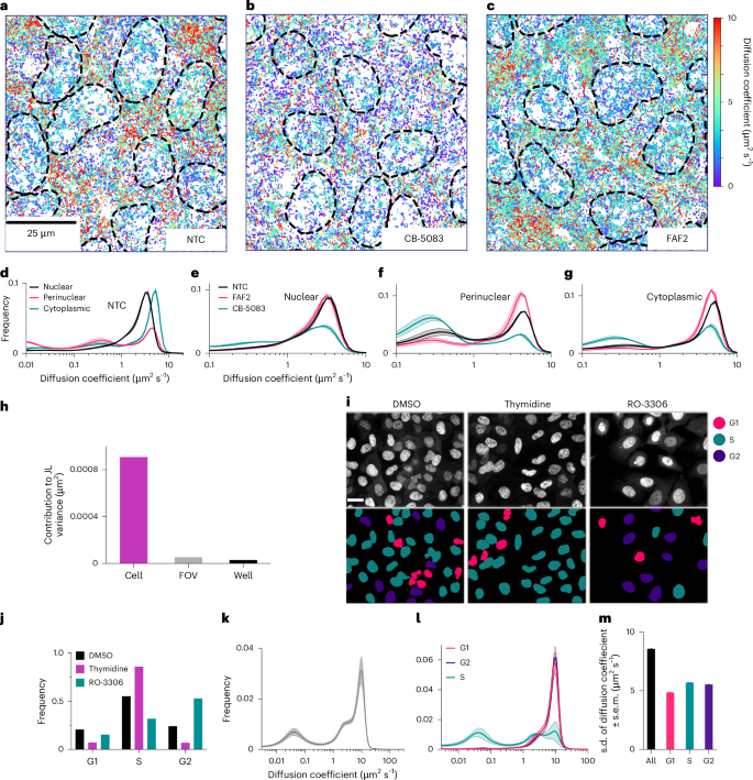
a–c, Representative image of trajectories, color coded by diffusion coefficient under NTC (a), the small-molecule inhibitor CB-5083 (b) and siRNA knockdown of the VCP cofactor FAF2 (c). Each condition is sampled from a minimum of 36 FOVs from 6 distinct wells and 2 biological replicates. d, State array analysis of NTC divided for each of nuclear, perinuclear and cytoplasmic compartments, illustrating the distinct mobility of VCP within each compartment. Shaded area represents the s.d. e–g, State array analysis of VCP perturbed with CB-5083 shows a drastic overall decrease in dynamics in the nuclear (e), perinuclear (f) and cytoplasmic (g), while FAF2 knockdown causes a more subtle effect that is predominantly a reduction in the prevalence of the slow subset of the perinuclear fraction (f). Each condition is sampled from a minimum of 36 FOVs from 6 distinct wells and 2 biological replicates. Shaded area represents the s.d. h, Top: analysis of sources of variance in SMT for KEAP1 measured under OLS illumination. i, Representative images of Halo-PCNA-labeled cells treated with 2 mM thymidine or 10 μM RO-3306. Bottom: cell cycle prediction from a machine learning (ML) model used to color cell by cycle phase. Scale bar, 25 μm. j, Quantification of fraction of cells in each cell phase in response to cycle block treatments in h. The following number of cells were analyzed for each condition: 34,067 for DMSO, 3,831 for RO-3306 and 6,044 for thymidine. k, State array analysis of total population of sparsely labeled PCNA cells. Shaded area represents the s.d. l, State array analysis for each of G1, G2 and S phases as predicted by the ML model. Shaded area represents the s.d. m, Single-cell-level s.d. of the diffusion coefficient for each cell cycle phase. Error bars denote the s.d. at the FOV level from 4,081 cells.
Using siRNA knockdown (Methods) of one well-characterized VCP cofactor, we highlight the ability of the OLS system to capture cofactor-specific and spatially dependent changes in protein dynamics. Here we achieve ~80% knockdown efficiency, characterized by western blot for the cytoplasmic and nuclear fractions (Methods) for FAF2 (also known as UBXD8; Fig. 2c–g and Extended Data Fig. 7g). We assess how a reduction in protein level for this cofactor affects local VCP dynamics. FAF2 is a protein that partitions between the ER and lipid droplets and has been identified as a member of the ERAD complex29. We observed an increase in diffusion within the perinuclear region by 13% with a diffusion coefficient of 3.00 μm2 s−1 (±0.19 s.d.), while VCP dynamics in the nucleus and the cytoplasm appear minimally disrupted with only a 2% decrease within each region. This measurement further confirms that the vast majority of VCP association to FAF2 takes place within the ER. This result highlights that the homogeneity of illumination, the FOV size and the presented segmentation model can enable the ability to measure differential activity of proteins in different cellular compartments or localizations.
SMT can be scaled in multiple dimensions: more trajectories per cell, more cells per FOV and more FOVs per well. Choosing optimal dimensions for scaling requires understanding which sources of variability limit the precision of downstream measurements. In assessing the consistency of SMT measurements (Methods), we determined that intercellular heterogeneity is the highest source of variance, exceeding FOV, well, plate or microscope-level variation. We found that cell-to-cell differences were at least an order of magnitude greater than FOV-to-FOV or well-to-well biases (Extended Data Fig. 7h–l). This strongly indicates that biological heterogeneity is dominant over technical variation of OLS-based SMT measurements (Fig. 2h). Examples of cell heterogeneity include cell cycle state, state of cell stress and genetic variation. Single-cell approaches such as large-FOV SMT can enable more nuanced measurements to better sample such heterogeneity30. We set out to exemplify such single-cell analysis by measuring the effect of cell cycle on PCNA protein dynamics. PCNA is involved in DNA replication and localizes to replication foci during S phase and exhibits distinct and specific protein dynamics across stages of the cell cycle31.
We introduced Halo-PCNA into U2OS isolated clones, resulting in sub-endogenous expression levels of tagged protein (Extended Data Fig. 8a,b) and found growth rates were not measurably affected by the expression of Halo-PCNA (Extended Data Fig. 8c). Proper localization of Halo-PCNA was confirmed with colocalization analysis with an RFP-labeled anti-PCNA ChromoTek Cell Cycle Chromobody (CCR) nanobody (Extended Data Fig. 8d).
Time-lapse microscopy was conducted on Halo-PCNA labeled with 50 nM JFX650, to achieve near-saturating labeling, for 12 h at 12 frames per hour (Extended Data Fig. 8e). A machine learning model was then trained using both manually assigned cell stages and time-based progression resulting in both a G1, S, G2 and mitosis classifier as well as a regression prediction across the continuum of the cell cycle (Extended Data Fig. 8f). The predicted cell cycle classification performed well as compared to manual annotation (Extended Data Fig. 8g). We also observed clear progression of individual cells through the cell cycle when regression prediction was plotted across the time series (Extended Data Fig. 8h and Supplementary Video 5). To further validate our cell cycle phase assignment model, we blocked cell cycle progression at S phases with thymidine or the G2–M transition with the CDK-1 inhibitor RO-3306 (refs. 32,33). Both treatments led to expected enrichment in the fraction of cells assigned to the respective cell phases (Fig. 2i,j). Cells were then labeled with 10 pM JF549 and 50 nM JFX650 to enable simultaneous cell cycle assignment based on near-saturating labeling along with SMT measurements. Two peaks of mobility were observed at 0.043 μm2 s−1 and 9.88 μm2 s−1, likely representing PCNA associated at sites of DNA replication and free PCNA, respectively (Fig. 2k). When cells in each cell phase were analyzed separately, it became apparent that the slow-moving population of PCNA was exclusively found in cells predicted to be in S phase, and that this subset of cells also showed a marked decrease in the fast-moving population (Fig. 2l). The standard deviation of the diffusion coefficient was then measured for 4,081 individual cells to characterize heterogeneity across the cell population, which is described in large part by predicted cell cycle state (Fig. 2m and Extended Data Fig. 8i). Taken together, these data provide an example of how large-FOV SMT enabled by OLS allows for the capture and elucidation of cell-level heterogeneity of protein dynamics.
OLS enables measurement of protein diffusion in solution
Due to the higher achievable frame rates and superior optical sectioning performance, we next wanted to test the suitability of OLS to measure the diffusive properties of purified proteins in solution. One could imagine such dynamics would be impacted by protein conformation, ligand interactions or PPIs. As modeled by the Stokes–Einstein equation, the movement of a particle is defined by the temperature and viscosity of the medium and the effective hydrated radius of the particle34. The effective hydrated radius is influenced by protein size, structure and physicochemical features of the protein surface. The diffusion of JF549-labeled His-Halo was measured with increasing concentrations of glycerol to modulate viscosity. A diffusion coefficient was estimated from tracking results and corrected using analytical expressions for tracking biases, resulting in a close match to the theoretical values predicted by the Stokes–Einstein equation (Fig. 3a,b and Methods).
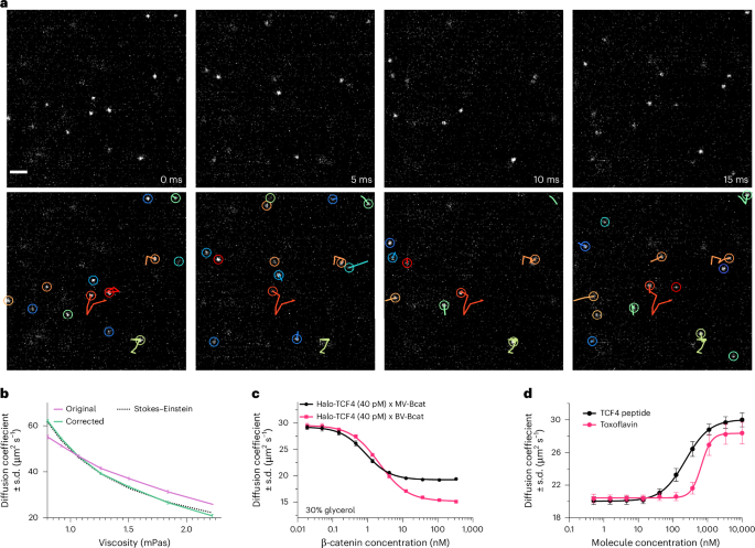
a, Representative sequential images of isSMT (top) with overlaid tracks (bottom) for JF549-labeled free HaloTag protein at 30% glycerol for a 192 × 192-pixel ROI at 200 Hz. Circles represent the detected PSFs; marks indicate the particle trajectories; color indicates the trajectory ID. Scale bar, 2 μm. b, Mean diffusion coefficient as a function of medium viscosity compared to theoretical Stokes–Einstein equation. 22–44-well replicates with four FOVs per well were acquired for each concentration at 200 frames per second, in duplicate 384-well plates from the same protein preparation. Error bars denote FOV-level s.d. c, Halo-TCF4 diffusion measured with a dose response of either monomeric (monovalent (MV)) versus dimeric (bivalent (BV)) β-catenin protein (Bcat); n = 8 wells. d, Diffusion coefficient of the TCF4–β-catenin complex measured across a dose response of unlabeled TCF4 peptide and toxoflavin; n = 32 FOVs from two distinct plates. Error bars denote the s.d.
Next, we sought to measure the change in diffusion mediated by PPIs. Transcription factor 4 (TCF4; 41.5 kDa) is known to bind with high affinity via its N terminus to β-catenin (85.6 kDa). We monitored JF549-labeled TCF4 diffusion at a concentration that enabled single PSF localization (40 pM) across a titration of unlabeled β-catenin and observed a concentration-dependent decrease in TCF4 diffusion with increasing concentrations of β-catenin (Fig. 3c and Supplementary Video 6). Interestingly, when a bivalent version of β-catenin was titrated in, TCF4 diffusion was shifted to a minimum of 15.08 µm2 s−1 versus 19.39 µm2 s−1 when monovalent β-catenin was added, consistent with a slower expected diffusion coefficient of a larger effective particle size. Next, we tested whether we could compete away the interaction between TCF4 and β-catenin with the addition of unlabeled TCF4. As expected, diffusion of the JF549-labeled TCF4 in complex with β-catenin was increased back to the level of JF549-labeled TCF4 by the titration of unlabeled competitive TCF4, suggesting competitive disruption (Fig. 3d). To demonstrate application of isSMT in the context of drug discovery, a small-molecule inhibitor and a TCF4 competing peptide were tested for their ability to alter the protein motion of JF549-labeled TCF4 in complex with β-catenin. Toxoflavin, a known inhibitor of β-catenin, was able to increase the diffusion of JF549-labeled TCF4 in a dose-dependent response with a maximum effect similar to the TCF4 competitive peptide (Fig. 3d)35. In summary, isSMT represents a new biophysical method for monitoring PPIs and protein–ligand interactions with potential sensitivity into the picomolar range.
OLS is amenable to a variety of SMLM techniques
The homogeneous illumination, high spatiotemporal resolution, imaging speed and overall robustness of the OLS system is likely to have broad advantages across multiple biological microscopy techniques. To demonstrate the ability to image SMT across two spectrally distinct fluorophores, we captured sequential time series of a JF549-labeled and a JF646-labeled Halo-KEAP1 resulting in clear single-molecule resolution across both wavelengths (Fig. 4a). KI-696 was dose titrated and the response was measured with both fluorophores (Fig. 4b). Importantly, despite a drop in sCMOS quantum efficiency in the far-red spectrum resulting in lower SNR (Extended Data Fig. 9a), we captured SMT data using the red-shifted JF646 and obtained EC50 values that were consistent with the brighter JF549 dye with measured EC50 values of 4.96 nM and 6.45 nM for JF549 and JF646, respectively. Robust measurement of protein dynamics with lower SNR is potentially explained by a minimal decrease in lower bound error rate (Extended Data Fig. 9b). Taken together, OLS-based SMT is likely to have applications in multicolor imaging and facilitates imaging of lower quantum yield fluorophores, broadening the palette of available fluorophores to measure protein motion across biological applications.
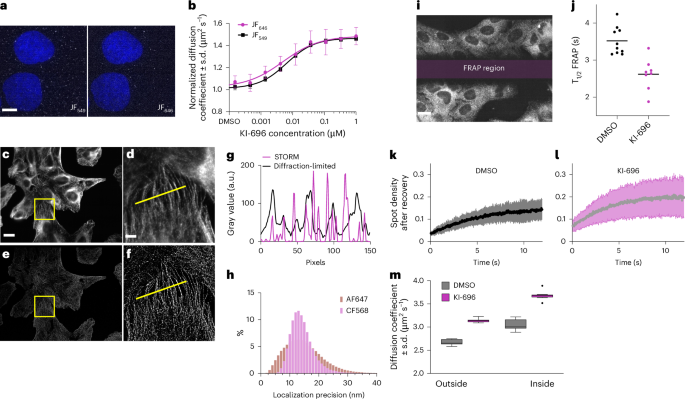
a, JF549 and JF646 co-labeled Halo-KEAP1 U2OS cells imaged within the same FOV. Scale bar, 5 μm. b, Ten-point dose response of KI-696-treated Halo-KEAP1 U2OS cells co-labeled with JF549 and JF646. c, Diffraction-limited image of a full OLS FOV of immunofluorescently labeled tubulin with AF647-conjugated secondary antibody (Methods). Scale bar, 20 μm. d, Zoomed-in region of interest from c. e, STORM reconstruction of full OLS FOV, as in c. f, Zoomed-in region of interest from e as in d. Scale bar, 5 μm. g, Line profile from yellow lines in diffraction-limited (d) and STORM (f) gray value (a.u., arbitrary units) to compare spatial resolution of microtubules. h, Localization precision histogram for AF647-labeled and CF568-labeled secondary antibodies used to stain microtubules with OLS illumination with a 0.4-ms integration time. i, Representative image of correlative FRAP/SMT where a central region is bleached using the OLS line scan before spot recovery after photobleaching. Areas outside and inside of the FRAP region are used to measure SMT. Scale bar, 20 μm. j, T1/2 FRAP for Halo-KEAP1 U2OS cells treated with DMSO or 1 μM KI-696 labeled with 400 pM JF549-Halo ligand. The black line denotes the median, and each spot represents an individual FOV from a single 384-well plate. k,l, Spot density after recovery over time for each of DMSO (10 FOVs; k) and 1 μM KI-696 (8 FOVs; l). Standard deviation shown in confidence bands for each condition. m, Diffusion coefficient from SMT for 400 pM JF549-Halo ligand concentration in bleached (inside) and unbleached (outside) region with 8 FOVs sampled for each condition. Whisker plots are rendered using the Tukey method with the median represented as a horizontal solid line.
We then investigated whether STORM imaging in fixed cells would result in images with high x,y resolution across a large FOV. Cells labeled with anti-tubulin primary antibodies and Alexa Fluor 647 (AF647) or CF568-conjugated secondary antibodies were imaged using STORM across a full ×60 FOV with a total imaging time of approximately 60 s (Fig. 4c–f and Supplementary Video 7). We observed that, despite the low integration time of 400 μs used in OLS, spontaneous photoswitching provided enough photons to achieve a lateral localization precision of approximately 15 nm using either AF647 or CF568 (Fig. 4g,h). Our results demonstrate the potential to conduct high-speed, high-throughput phenotypic screening with STORM or other SMLM techniques with OLS illumination.
Next, we leveraged the line scan component of OLS to conduct a correlative SMT-fluorescence recovery after photobleaching (FRAP) experiment on KI-696 treated Halo-KEAP1 cells labeled with JF549. We bleached a 240 × 40 μm2 region by focusing the scan region on a narrow subset of the FOV for a duration of 100–200 sweeps before acquiring the full FOV under normal SMT acquisitions (Methods). This resulted in each frame containing a bleached (FRAP region) and an unbleached (Fig. 4i and Supplementary Video 8) region. Instead of capturing the intensity recovery after photobleaching over time, the normalized spot density after recovery was measured (Fig. 4k,l). We measured an average T1/2(DMSO) of 3.52 s (±0.38 s.d.) and T1/2(KI-696) of 2.27 s (±0.43 s.d.) at a JF549 dye concentration of 400 pM (Fig. 4j). These results are consistent with our reported SMT measurements and indicate that KI-696 increases Halo-KEAP1 protein dynamics. To further ascertain the consistency of our FRAP measurement, we applied SMT to both bleached and unbleached regions of the FOV. In both cases, we were able to measure an increase in Halo-KEAP1 dynamics under a 1 μM KI-696 perturbation at a range of dye concentrations (Fig. 4m and Supplementary Fig. 10c). These results highlight and confirm that the advantageous properties brought upon by OLS in combination with the presented tracking algorithm enable sensitive spot detection and SMT even when labeling sparsity is not optimized for.
These data demonstrate that the large FOV, OLS scanning, and high SNR with fast integration times enabled two-color SMT, STORM and FRAP to be implemented with scale, speed and consistency. We anticipate that our platform will be compatible with other approaches such as fluorescence correlation spectroscopy (FCS) and image correlation spectroscopy (ICS) and could enable leveraging such advanced microscopy methods in high-content applications.
Discussion
We have demonstrated how OLS, as a new illumination scheme, enhances several properties of SMLM and SMT-based techniques. Compared to previously described illumination methods applied to SMLM and SMT, OLS provides a large and homogeneously illuminated FOV, finer sectioning ability, superior SNR and high spatiotemporal resolution. We demonstrate OLS illumination implemented on four distinct microscopes, highlighting the robustness and consistency of the systems. The improvement in rejecting out-of-focus light enables better single-molecule detection and localization, making OLS suitable for conducting SMT on a variety of cellular systems and protein targets where, previously, background fluorescence would be limiting. The data presented herein allow us to anticipate achieving high SNR SMT results in more complex cellular systems such as spheroid cultures from immortalized cancer cells.
OLS enables data acquisition at frame rates up to 1,250 Hz without compromising SNR and tracking fidelity. As illustrated with Halo-KEAP1, a frame rate of 400 Hz is required to fully characterize the increase in diffusion of drug-induced release from NRF2. We anticipate that there are many biological processes that involve rapid protein motion that were previously unmeasurable with other SMT illumination methods. OLS will provide an opportunity to tackle new protein and cellular mechanisms that are likely occurring at the sub-millisecond scale. Nonetheless, in this current implementation, imaging speed comes at the expense of FOV size, which past a certain size reduction, will prevent the capture of full cell objects. Mitigation strategies using optimized hardware solutions such as cameras with improved speeds are worth further investigating in this area.
By conducting SMT measurements on a multifaceted and spatially regulated protein such as VCP, we illustrate the ability of OLS to capture small but significant spatially dependent changes in diffusion coefficients. Being able to accurately measure protein motion as it relates to intracellular function can help gain a more nuanced understanding on the prevalence and importance of protein cofactors.
Our analysis suggests that the greatest source of variation in SMT measurement stems from cell-to-cell heterogeneity with respect to protein motion. The large FOV enabled by OLS allows for the simultaneous capture of upwards of 70 U2OS cells in culture, enabling the capture of inter-cell heterogeneity. This was exemplified with PCNA where we were able to simultaneously assign the cell cycle phase and monitor protein dynamics. We show that PCNA protein dynamics are slower during S phase, which correlates to protein enrichment at sites of DNA replication. During G1, G2 and M phases, we observed a robust increase in dynamics corresponding to the majority of PCNA being homogeneously distributed throughout the nucleus. These findings are consistent with previous characterization of PCNA dynamics31 but there are important improvements in the approach presented here. Cell cycle was predicted computationally through machine learning models using localization of PCNA as opposed to manual assignment. Additionally, our OLS platform enabled rapid and automated capture and analysis of thousands of cells versus tens of cells per condition typically analyzed using manual SMT approaches. When characterizing protein motion in heterogeneous cell populations and potential rare cell subtypes, automated cell classification along with scaled SMT data collection and analysis will be critical to enable work that is comparable with flow cytometry and other single-cell analysis techniques.
Given the versatility of OLS, we were able to apply SMT to directly study protein dynamics in solution. Despite the intrinsic difficulty in generating trajectories for fast-diffusing proteins in solution, we validated isSMT measurements by showing a strong overall agreement between experimental measurements and the corresponding Stokes–Einstein theory. We demonstrated the method’s relevance by measuring the interaction between TCF4 and β-catenin. We also demonstrated the ability to leverage isSMT to monitor the disruption of this protein interaction with a competitive peptide and small-molecule inhibitors, suggesting that there could be relevant application in drug discovery. Importantly, isSMT requires picomolar concentrations of purified protein enabling assay development of difficult-to-purify proteins and the sensitivity to measure sub-nanomolar affinities. By contrast, competing techniques such as FCS, FRAP or temporal analysis of relative distances (TARDIS) typically fit a model to an ensemble average over all dynamical states present in the sample, limiting the ability to distinguish multiple motion states of a given protein in solution. Additionally, FCS and FRAP are usually performed at emitter concentrations that are orders of magnitude greater than what is suitable for tracking approaches. Tracking can give precise diffusion coefficient characterizations at low concentrations and is preferable for situations where it is inconvenient or impossible to use high molecule concentrations. We speculate that ligand interactions can alter protein diffusion in ways beyond those caused by disruption of PPIs, including ligand-induced confirmational changes, protein stability changes and perhaps more subtle changes to protein hydration shell resulting in small but measurable changes in diffusion.
We highlighted the versatility of OLS beyond SMT by demonstrating its suitability for rapidly capturing STORM datasets, despite very low illumination and integration times, and achieving a lateral resolution of ~15 nm for both AF647 and CF568. Finally, we demonstrated a correlative SMT/FRAP approach by which to study protein diffusion. This simultaneous acquisition may enable the measurement of protein dynamics at different timescales allowing for the capture of a wider range of protein dynamics comprising discrete but biologically important subpopulations. As with SMT, we expect OLS to enable large-scale advances in microscopy studies that benefit from high resolution, homogeneous and rapid stroboscopic illumination, and rapid frame rates. We recognize that data storage and processing of large datasets generated by capturing time series of multiple large FOVs can be infrastructurally prohibitive. However, as phenotypic imaging becomes central to systems biology studies and drug screening, we expect an increase in demand for more advanced microscopy technologies that enable more sophisticated assays such as OLS.
Here, we provide an initial characterization of the broad utility and ease of implementation of OLS using a series of experimental setups. However, this minimal set of experiments is not a comprehensive description of the utility of OLS; rather, it is the ease of implementation of OLS, coupled with this experimental flexibility, that will provide the research community with a valuable tool to bring SMLM to bear on many dynamic biological systems20,21,22,36,37,38,39,40,41,42.
Methods
OLS microscopy
SMT image acquisition for OLS datasets was performed on a custom-built microscope based on a Nikon Ti2, motorized stage, stage top environmental chamber (OKO Labs), quadband filter cube (Chroma), custom laser launch with 405 nm, 561 nm and 642 nm wavelengths, delivering >10 mW, >150 mW and >150 mW of power to the back focal plane of the objective, respectively. The custom laser launch consists of three externally triggerable free-space laser sources (Cobolt 06-MLD; Huebner Photonics; 2RU-VFL-P-2000-560-M; MBP Communications; VFL-P-2000-642-M; MBP Communications).
The OLS (Extended Data Fig. 1a and Supplementary Fig. 1d) unit is attached to the back port of the microscope providing optical excitation and scanning. The OLS unit receives collimated Gaussian-shaped optical excitation via a polarization-maintaining single-mode fiber coupled to a laser beam coupler. The laser excitation is sent through a combination of a Powell lens, custom-designed cylindrical lenses, and an achromatic lens to shape the beam into a laser line. The beam is guided over a set of two position-adjustable right-angle prisms followed by an aspherized achromatic lens to position the beam and focus the scan axis onto galvanometric scanning mirrors, which is adjusted to position the beam at an offset of 3.8 mm to the central optical axis in the objective’s back focal plane to achieve an illumination light sheet in the sample at an inclination angle of 60° (Extended Data Fig. 1e).
Fluorescence emission is passed through a high-speed filter wheel (Sutter Instruments) and collected with a back illuminated sCMOS camera (ORCA-Fusion BT, Hamamatsu). The sCMOS camera is operated in progressive mode with an exposure time of 407 µs at an internal line interval of 4.87 µs to achieve a virtual rolling slit of ~200% of the optical excitation and fluorescence line width (Extended Data Fig. 1f). Images were acquired with a ×60 1.27-NA water-immersion objective (Nikon). The environmental chamber was set to 37 °C, 95% humidity and 5% CO2.
The default optical excitation is set to an average power of 250 mW at the back focal plane of the objective. Given the 90% transmission of the equipped objective lens for a wavelength of 561 nm, operating the laser at 100 Hz with a duty cycle of 90% for a 100-fps acquisition yields a peak power of 250 mW or a pulse energy of 2.25 mJ per pulse in the sample plane. Assuming a non-scanned line, at an angle of inclination of 60° and with an excitation line adjusted to 280 µm in the focal plane (that is, 12.5% wider than the FOV to ensure homogeneous and complete coverage), the peak power density and the peak energy density can be estimated at 25.77 kW/cm2 and at 231.9 J/cm2, respectively. Considering a scanned line at 22.2 µm ms−1, the local effective optical excitation per position in the sample can be estimated at 1.85% of the entire optical excitation by scanning across the entire FOV, which subsequently leads to an instantaneous and local average peak power density and instantaneous and local average peak energy density of 476 W/cm2 and 4.29 J/cm2, respectively.
System hardware control is realized in a custom-designed and user-configurable electric circuit board for software interfacing, synchronization and device control. Data acquisition control is realized in a custom-designed and user-configurable acquisition script in MicroManager for raster scanning 384-well plates, a custom-designed automated focusing routine (Extended Data Fig. 1b). One frame of Hoechst and Potomac Red channel were collected at the same frame rate for downstream registration of trajectories to nuclei and cytoplasms, respectively.
HILO microscopy
SMT image acquisition for HILO datasets was performed on a custom-built microscope based on a Nikon Ti2, motorized stage, stage top environmental chamber (OKO Labs), quadband filter cube (Chroma), custom laser launch with 405 nm and 561 nm wavelengths, delivering >10 mW and >150 mW of power to the back focal plane of the objective, respectively. Fluorescence emission was passed through a high-speed filter wheel (Finger Lakes Instruments) and collected with a backlit sCMOS camera (ORCA-Fusion BT, Hamamatsu). Images were acquired with a ×60 1.27-NA water-immersion objective (Nikon). The environmental chamber was set to 37 °C, 95% humidity and 5% CO2. For each FOV, 150 SMT frames were collected at a frame rate of 100 Hz, with a 2-ms stroboscopic laser pulse.
SNR definition and quantification
SNR is defined based on the likelihood ratio for a hypothesis test comparing: a target-absent condition, where the local image is modeled by the sum of a constant offset, and independent Gaussian-distributed noise; and a target-present condition, where the local image is modeled by the sum of a centrally located Gaussian peak (with known width but unknown amplitude), independent Gaussian-distributed noise and a constant offset. Following the method described in ref. 43, the SNR is expressed as
where:
-
A is the image, cropped to the current region of interest (ROI);
-
ws is the side length, in pixels, of the square ROI;
-
(circledast) is the inner product operator;
-
hG is a zero-mean detection kernel, matched to the expected Gaussian target profile, and with (sum {h}_{G}^{2}=1) where the summation is taken over the ROI;
-
hu is a uniform kernel (that is, it has a value of 1 over the entire ROI).
SMT software
An example dataset, software packages and instructions have been included as Supplementary Information. This package enables a user to reproduce the analysis of spot identification, tracking and stay array analysis. More details describing mindlt–release 1.0.0 (Supplementary File 1) are provided in the subsequent sections.
SMT methods
SMT data were processed with a custom pipeline operating on image sequences produced by the microscope (Extended Data Fig. 2). Briefly, individual emitters were detected by applying a generalized log-likelihood ratio test to every 11 × 11 pixel subwindow in the image as described above (SNR definition and quantification)43. We detected emitters by identifying pixels with a log-likelihood ratio exceeding 14 (for cellular SMT) or 16 (for isSMT). Detected emitters were localized to subpixel precision in a two-stage procedure. First, the subpixel location was estimated by computing points of maximum radial symmetry44. Second, this estimate was used to seed an iterative Levenberg–Marquardt fitting routine to a two-dimensional (2D) integrated Gaussian within an 11 × 11-pixel subwindow centered on the detection45,46.
Localized emitters were linked in time to produce trajectories using a modification of Sbalzarini’s hill-climbing algorithm47,48. In all SMT, we prohibited links longer than 1.25 µm for cellular SMT (2.5 µm for isSMT) and links over more than two gap frames to limit association error. Emitters were assigned to segmentation categories (nucleus, cytoplasm) by comparing their subpixel location with the semantic masks produced by the segmentation routine. See demo software and data available on Zenodo via https://doi.org/10.5281/zenodo.14026442 (ref. 49). To recover diffusive subpopulations from observed SMT tracks, we rely on variational Bayesian mixture modeling techniques. These methods resolve a distribution over diffusion coefficient given observed trajectories while accounting for the uncertainty from the localization error, and can be combined with segmentation to generate compartment-specific distributions. While scalable to the large datasets generated by OLS, these techniques do not take into account confinement effects, local environmental anisotropy (for example, the orientation of the cell membrane) nor superdiffusive motion (for example, directional motion by cytoskeletal motors). Accounting for these effects in a manner compatible with large datasets produced by OLS imaging is an attractive area for future studies.
Measurements on trajectories
When reporting the number of trajectories, we excluded singlets (trajectories with one detection), as these do not contribute information to most dynamical estimates.
Average diffusion coefficients were computed with the mean squared displacement method (Dest = MSD2D/4∆t)47,50. This estimator is expected to overestimate the diffusion coefficient by σloc2/∆t, where σloc2 is the variance of the one-dimensional (1D) localization error and ∆t is the frame interval.
To resolve trajectories in multiple dynamical states, we inferred the coefficients of a Brownian mixture model over a grid of diffusion coefficient values and localization error values using state arrays, a variational Bayesian routine based on the Dirichlet process mixture26,51,52. Mixture components were selected as the Cartesian product of 100 diffusion coefficients log-spaced between 0.01 µm2 s−1 and 100 µm2 s−1 and 31 localization error values from 0.02 µm to 0.08 µm (1D standard deviations). Occupations are reported as the mean posterior probabilities of each diffusion coefficient marginalized over all values of localization error. To make inference tractable, we limited inference to 10,000 trajectories randomly sampled from each well.
Bias estimation in single-population samples was performed using analytical calculations that capture the probability of false linking and jump-length (JL)-distribution truncation due to a finite search radius.
For isSMT, spatial locations are uniformly distributed, allowing the probability of false linking to be estimated based on the observed emitter concentration and a nearest-neighbor linking model. This probabilistic analysis also allows characterization of the false-link jump-length distribution. Single-population bias estimates incorporate these false-linking artifacts, and the prohibition on jump-length observations greater than the search radius. As shown in Fig. 3b, these bias expressions are used to improve diffusion coefficient estimation accuracy.
Empirical estimate of linking precision
To estimate the accuracy of the linking algorithm, we used a bootstrapping procedure. Detections from the first and second halves of the movie were superimposed, and the tracking algorithm was run on the resulting set of detections while blinded to the origin of each detection. From this, we computed the fraction of links generated where individual detections were joined from different halves of the movie. Since this fraction accounts neither for erroneous links between detections in the same half of the movie nor for the effects of photobleaching, it forms a lower bound on the linking error rate.
Estimate of SMT dynamic range
To estimate the impact of frame rate on SMT dynamic range (Extended Data Fig. 5), we considered the bounds on the possible values of the MSD estimator of the diffusion coefficient ((hat{D})) for a Brownian particle with Gaussian localization error. The MSD estimator is biased upwards by localization error according to (hat{D}=D+{sigma }_{{loc}}^{2}/Delta t), where ({sigma }_{{loc}}^{2}) is the variance of the 1D localization error and (Delta t) is the frame interval. Because (D) is nonnegative, this yields (hat{D}ge {sigma }_{{loc}}^{2}/Delta t). In the opposite limit, when the true jumps of the particle are much larger than the search radius R used for tracking, the jumps are uniformly distributed within the tracking range gate (a circle of radius R) and the MSD estimator of the diffusion coefficient is capped at ({R}^{2}/8Delta t). Together, this yields the dynamic range estimate ({sigma }_{{loc}}^{2}/Delta tle hat{D}le {R}^{2}/8Delta t). Consequently, the effect of changing frame rate is to translate the dynamic range in the (log hat{D}) domain. This simple model of dynamic range does not consider the impact of trajectory misconnection (which may change the upper bound) or the non-MSD estimate of diffusion coefficient in state arrays (which may reduce the lower bound).
Optical–dynamical simulations
To evaluate tracking methodology and the impact of frame rate on SMT dynamic range, we performed optical–dynamical simulations. These simulations use a scalar diffraction approximation to a paraxial imaging system with NA = 1.2 (ref. 53). Briefly, we first simulated discrete mixtures of Brownian motions without state transitions at frame rates of 12.5, 25, 50, 100, 200, 400, 800 or 1,600 Hz in a cuboid with dimensions 45 × 45 × 8 µm3 (XYZ). Particles were initialized at a density of 0.31 or 0.62 particles per cubic micrometer (depending on the simulation), and were subject to photobleaching at probability 0.03 per frame. Positions of particles coinciding with 500-µs pulses (modeling the stroboscopic illumination in HILO or the rolling shutter in OLS) were accumulated onto a simulated 2D camera via convolution with the system’s 3D PSF. This yielded a probability distribution of photon arrivals over all simulated camera pixels. Next, we sampled photon arrivals from this distribution as a Poisson process up to a mean of 90 or 125 photons per particle (depending on the simulation). Finally, Gaussian read noise with a root mean square of three photons was added, we multiplied this by a 4.3 counts-per-photon gain factor, and the movie was discretized into 16 bits. We then subjected this movie to tracking and state array inference with settings identical to those of Halo-KEAP1 tracking.
Assessment of highest source of variance from experiment: jump resampling experiment
To evaluate the contribution of well-to-well, FOV-to-FOV and cell-to-cell biases on estimated mean 2D jump length, we acquired a full plate (308 wells) of HILO and OLS data with DMSO-treated KEAP1-HaloTag labeled with JF549 at 100 Hz. After excluding the outer ring of wells in the 384-well plate, this yielded a dataset with 308 wells, 12 FOVs per well, and a mean of ~44 cells per FOV (for OLS) or ~15 cells per FOV (for HILO). We considered a simple model of jump length. Letting Y be the observed 2D jump length, we modeled Y as the sum
Bwell, BFOV and Bcell are random variables modeling bias at the well, FOV or cell levels, respectively, and X models the intrinsic stochasticity in jump length conditional on a particular well, FOV and cell. The simplification is that Bwell, BFOV, Bcell and X are assumed to be independent. Under this simplification, Var(Y) = Var(Bwell) + Var(BFOV) + Var(Bcell) + Var(X). A more physically realistic model would take into account the potential dependencies between these random variables.
To estimate Var(Bwell), Var(BFOV), Var(Bcell) and Var(X), we computed the variance in sample means for four different jump resampling schemes:
-
1.
Sample N jumps from the whole plate. The resulting sample mean averages over all sources of variability (Bwell, BFOV, Bcell and X).
-
2.
Sample a well, then sample N jumps from that well. The resulting sample mean averages over BFOV, Bcell and X, and the variance over these sample means is expected to approach Var(Bwell) as N becomes large.
-
3.
Sample a well, sample an FOV from that well, then sample N jumps from that FOV. The resulting sample mean averages over Bcell and X, and the variance over these sample means is expected to approach Var(Bwell) + Var(BFOV) as N becomes large.
-
4.
Sample a well, sample an FOV from that well, sample a cell from that FOV, then sample N jumps from that cell. The resulting sample mean averages over X only. The variance over these sample means is expected to approach Var(Bwell) + Var(BFOV) + Var(Bcell) as N becomes large.
One thousand rounds of sampling were performed for each sampling scheme and the variances of the biases Bwell, BFOV and Bcell were estimated by the difference between the variances over sample means produced by each resampling scheme. As expected, only Var(X) depended on the sample size N and the other sources of variability were stable with respect to the sample size after ~100 jumps (Extended Data Fig. 7).
His-Halo sample preparation
His-Halo was diluted to 50 pM in imaging buffer consisting of 25 mM HEPES pH 7.4, 150 mM NaCl, 1 mM dithiothreitol, 0.03% (wt/vol) BSA, 0.01% NP-40, with glycerol levels spanning 0% to 40%. Dilutions were transferred to a 384-well plate, which was incubated at 37 °C for 15 min before imaging using OLS. We captured 22–44-well replicates per concentration and acquired four FOVs per well at 200 frames per second, and the glycerol titration experiment was performed on two plates using the same protein preparation viscosity calculations performed following previously described methods54,55.
β-catenin–TCF4 sample preparation
GST–β-catenin (dimer β-catenin) was made via bacterial expression. The GST tag was removed via thrombin cleavage and purified by size-exclusion chromatography to obtain monomer β-catenin.
His-Halo-TCF4 (1–53) was made via bacterial expression, then labeled with JF549 and purified by size-exclusion chromatography. The final concentration was determined via Nanodrop and gel band intensity imaged on the Cy3 channel of ImageQuant 800.
Halo-TCF4 and β-catenin were diluted in imaging buffer (25 mM HEPES-K pH 7.6, 0.1 M EDTA pH 8.0, 12.5 mM magnesium chloride, 100 mM potassium chloride, 0.2 mM PMSF, 1 mM dithiothreitol, 0.3 mg ml−1 BSA, 0.01% NP-40 and 30% glycerol, pH 7.9) to final concentrations of 40 pM and 30 nM, respectively. Compounds were printed onto a 384-well CellVis glass-bottom plate via Echo 655, then incubated with β-catenin for 10 min at room temperature before addition of Halo-TCF4. Protein solutions were dispensed using an Integra VIAFLO. Plates were then incubated at 37 °C for 2 h before imaging.
STORM and PALM datasets
U2OS cells were fixed in 4% paraformaldehyde for 10 min, washed three times with PBS, permeabilized with 0.1% Triton-X for 10 min and washed again three times with PBS. Cells were then blocked in 2% BSA for 1 h at room temperature followed by overnight incubation with anti-alpha tubulin antibody (ab7291) at 4 °C. The primary antibody was removed by washing three times with PBS and cells were blocked again with 2% BSA for 1 h at room temperature. Alexa Fluor 647-conjugated secondary antibodies were diluted at a 1:1,000 ratio in blocking buffer and incubated for 2 h at room temperature. Cells were then washed three times with PBS to remove excess secondary antibody. Hoechst 33342 was added at a concentration of 7 μM with the secondary antibodies for nuclei visualization.
Photoswitching buffer for STORM imaging was prepared as previously described56.
Buffer A was prepared with 0.5 ml 1 M Tris (pH 8.0), 0.146 g NaCl and 50 ml of H2O. Buffer B was prepared with 2.5 ml 1 M Tris (pH 8.0), 0.029 g NaCl, 5 g glucose and 47.5 ml of H2O. GLOX solution was prepared by mixing 14 mg Glucose Oxidase (G2133) and 17 mg ml−1 of Catalase (C40) with 200 µl of Buffer A. The final photoswitching buffer was prepared by combining 100 μl 1 M MEA (M9768) with 10 μl of GLOX and 1 ml of buffer B. This buffer was added to cells in the 384-well plate before imaging.
Low laser power (300 mW) was used to capture diffraction-limited images and identify the pertinent focal plane. Laser power was increased to achieve ~500 mW at the back focal plane to initiate photoswitching. Around 500–5,000 frames were acquired, with an integration time of 400 μs.
Line FRAP acquisition
FRAP datasets U2OS-KEAP1 were recorded by consecutively imaging five pre-bleaching frames, bleaching a subregion of the imaging FOV and capturing fluorescence recovery at an operating frame rate of 25 fps. Bleaching a FOV subregion was achieved by scanning the excitation laser for 100–200 sweeps across a subregion of the FOV (16–25% FOV height, 100% FOV width) at high laser power (300 mW) to bleach the local fluorescence. Fluorescence recovery was acquired with 400–500 frames following the bleaching step at low laser power (70 mW). Modulating the laser power was achieved by implementing an Acousto-Optical Tunable Filter in the laser engine module (AOTF-Ed 2018–1; Opto-Electronic) adjusted for a bleaching and imaging power of the system’s 560-nm excitation.
Cell segmentation
Segmentation models were trained to segment specific compartments from the Hoechst and Potomac Red images. The models were trained using a U-Net architecture with the following class-balanced entropy loss57,58.
Where:
-
z is the predicted output of the model for all classes
-
C is the total number of classes
-
b is a hyperparameter between 0 and 1
-
ny is the number of training samples per class y
For the Hoechst model, three classes were used representing nuclei, nuclear border and autofluorescence artifacts. For the Potomac Red model, five classes were used representing nuclei, cytoplasm, nuclear border, cell border and autofluorescence artifacts.
Cell cycle classification model
A segmentation model was trained to identify nuclear regions. The input is an image of JF549-labeled PCNA and the model generates pixel-level classifications. In addition to identifying and generating mask objects for the nuclei, each nucleus is categorized as being within one specific phase of the cell cycle. From fluorescently labeled PCNA images, we were able to categorize the nuclei using the following labels: mitotic (M), growth 1 (G1), early S, mid S, late S (S) or growth 2 (G2).
To evaluate the cell cycle prediction model, we compared the nuclei categorical predictions to manually labeled data (Supplementary Fig. 8). Once the pixels that correspond to each category have been identified, we can compute tracking metrics within each mask object.
Perinuclear fraction segmentation
To identify the perinuclear fraction, an intensity-based segmentation method was applied. For each plate, a flat field correction matrix was computed by fitting the mean across all FOVs to a fourth-order polynomial. Each FOV was then corrected by dividing by this matrix. The resulting images were convolved with a Gaussian kernel with a sigma of ten pixels (~1.083 µm). The relevant perinuclear areas were then identified by selecting the pixels with an intensity greater than or equal to the 80th percentile for each FOV. The non-perinuclear area of the cytoplasm was defined as (Cwedge {neg P}) where C is the cytoplasmic mask generated from the Potomac Red segmentation model detailed above and P is the perinuclear fraction mask.
Reporting summary
Further information on research design is available in the Nature Portfolio Reporting Summary linked to this article.
Responses