A 1 km monthly dataset of historical and future climate changes over China

Background & Summary
Climate data, such as the basic climate variables of temperature, precipitation, and radiation, and further developed bioclimatic variables of seasonality and evapotranspiration, are widely used in meteorology, hydrology, agriculture, and ecology1,2,3,4,5. In the context of rapidly changing climate, historical changes and future projections are two important parts for climate datasets to enhance data consistency and applicability6,7. Meanwhile, climate data with high resolution are preferred for capturing subtle changes, and are further used to better understand the profound impacts of climate change on natural and social systems8,9.
Common methods to obtain the required climate data include interpolation10,11 and downscaling12,13, to facilitate studies at a fine scale by converting point-based or reanalysis products into higher-resolution data. Observation records from meteorological stations are reliable sources of historical climate data. However, studies are always constrained by limited amount and uneven distribution of meteorological stations14, which highlights the necessity of interpolation. The Australian National University Spline (ANUSPLIN) is professional software to interpolate climate data based on the georeferenced algorithms called the thin plate smoothing splines (TPSS)15,16. The TPSS algorithm can be viewed as a generalization of standard multi-variate linear regression, so that the ANUSPLIN can perform multi-surface fitting simultaneously with the introduction of different covariates16. Compared with traditional interpolation methods such as ordinary Kriging and inverse distance weighting10, TPSS, due to its superiority in capturing the impacts of topography on climate, has been widely used for spatial interpolation of various climate variables, such as temperature17, precipitation11, and radiation18, and has also been used for the development of global datasets such as the CRU high-resolution gridded datasets19 and WorldClim20.
Future climate data are mainly derived from general circulation models (GCMs). However, biases always exist due to scenario setting, model choice, and internal climate variability among different GCMs, which can be corrected by downscaling13,21. Currently, statistical and dynamical downscaling methods are widely applied. The statistical downscaling assumes that the statistical relationship between large-scale and local climate variables remains stable under future climate scenarios22, while the dynamical method is based on the regional climate models with initial boundary values provided by GCMs23. Therefore, statistical downscaling is suitable for long-term averaged climate data while saving calculating resources13,22. Delta correction (DC), an easily operable statistical downscaling method, can be implemented by calculating the anomaly (i.e., delta change) between historical and future climate data and then applying the anomaly to the baseline data12,24. The DC method has presented robust performance under the background of future scenario12, historical period25, and even paleoclimate reconstruction26, at global12, national27, and regional28 scales. Some widely used databases have also been developed based on DC method, such as the WorldClim20 and Chelsa3.
China has a large territory with diverse terrain and complex climate systems, making it difficult to obtain high-resolution climate data29. Also, most meteorological stations in China are established after 1950, resulting in the deficiency in long-term observation data30. Therefore, research on the long-term climate change and its impacts across China is limited. Recently, some climate datasets for China have been developed, such as the monthly temperature and precipitation during 1901–201725, the precipitation variability during 1961–201511, and the evapotranspiration during 1981–201531. However, only a few of them contain long-term averaged climate data including a variety of variables covering historical and future periods.
In this study, a bias-corrected 30-year averaged monthly climate dataset was developed at 0.01° × 0.01° (≈1 km × 1 km) grid using ANUSPLIN software and the DC method, based on the latest observation records from meteorological stations in China and GCMs. The dataset includes 28 commonly used climate variables during the historical period of 1991–2020 and future periods of 2021–2040, 2041–2070 and 2071–2100. It was evaluated using the interpolated and downscaled outputs, to ensure data reliability and provide a high-quality long-term averaged climate dataset for climate change impact research.
Methods
Data acquisition
Historical observation dataset
The 30-year averaged surface standard climate dataset for 1991–202032,33, the baseline year in this study, was recently released based on the observed records of 2185 meteorological stations (Fig. 1). The dataset provided six types of climate variables including temperature, precipitation, humidity, air pressure, wind, and radiation. We selected five basic variables (Table 1), including monthly precipitation (pr), mean air temperature (tas), minimum air temperature (tasmin), maximum air temperature (tasmax) and mean percentage of sunshine (sunp). These variables, along with the bioclimatic variables developed based on them, are commonly used in the research of climatology and ecology1,3,7,20. All the 2185 stations provided records of the variables tas, tasmax, tasmin, and pr, and 2093 stations with the records of sunp (Fig. 1). The generation of 30-year averaged monthly climate data followed the guidance of China Meteorological Administration34 and World Meteorological Organization35, to ensure the quality of this observation dataset in compliance with national and international standards.

The distribution map of meteorological stations in China. Common stations (N = 2093) meant stations with data of all the five basic variables. Extra stations (N = 92) meant stations with data except for the percentage of sunshine.
GCM selection
The Coupled Model Intercomparison Project Phase 6 (CMIP6), overseen by the World Climate Research Programme’s Working Group on Coupled Modelling, is a major international multi-model research activity coordinating historical and future climate data from different GCMs36. Among its various climate products, the historical simulations for 1850–2014 are commonly used. It also provides climate projections for 2015–2100, based on different scenarios of future emissions and land use changes, namely, the Shared Socioeconomic Pathways (SSPs)37.
We used historical simulations (1951–1980, 1991–2014) and future projections (2021–2040, 2041–2070, 2071–2100) from nine GCMs under three scenarios, namely, SSP1-2.6, SSP2-4.5, and SSP5-8.5 (Table 2). To maintain consistency with variables in our historical observation dataset, these GCMs also included monthly data of tas, tasmax, tasmin, pr, and the total cloud cover (clt, i.e., 100 − sunp, for convenience of calculation, following Wang et al.38). This partly restricted our selection of GCMs, as only a limited number of GCMs provided clt data. We further considered the GCMs selected by widely used databases developed based on CMIP6 data, such as the WorldClim20 (https://worldclim.org) and Chelsa39 (https://chelsa-climate.org). As for the SSPs, SSP1-2.6, SSP2-4.5, and SSP5-8.5, the continuations of the RCP2.6, RCP4.5, and RCP8.5 forcing levels in CMIP5 representing low, medium, and high forcing categories, indicated optimistic, moderate, and pessimistic future emission scenarios, respectively37,40. All the CMIP6 data were downloaded from the data search interface (https://aims2.llnl.gov/search/cmip6/).
Generation of high-resolution historical observed data
Due to the coarse spatial distribution of meteorological stations, interpolation was first required to convert the historical observation dataset during 1991–2020 at geographic coordinates into high-resolution surface data. The interpolation software ANUSPLIN v.4.4 was applied to generate 12 monthly surfaces at a resolution of 0.01° × 0.01° (≈1 km × 1 km) for each variable. In this study, we set longitude and latitude as independent variables, and used elevation as a third independent variable for tas, tasmax, tasmin, and pr to perform full tri-variate spline function. The elevation data were derived from the Shuttle Radar Topography Mission digital elevation model41, whose original resolution of 90 m was resampled to 0.01° using the bilinear method in this study. For sunp, monthly pr data were used as surface independent covariate, as incorporating the dependence on rainfall allowed for a better representation of complex solar radiation patterns16,42.
Based on the five interpolated basic variables, 23 bioclimatic variables were further calculated (Table 1). Bio1 to Bio19 were developed to describe specific bioclimatic conditions and thus widely applied in the study of biology and ecology43,44,45. The variables tas, tasmax, tasmin, and pr were required for the calculation of these 19 bioclimatic variables. Unlike Worldclim, which uses the average of tasmax and tasmin to represent monthly mean temperature44, we instead applied updated equations to use tas directly, following Karger et al.3. Bio20 to Bio23 were calculated using tas, pr, and sunp as input into the modified bioclimatic envelope model38,46 developed from a simple process-based bioclimatic model (STASH)47. The general algorithm of STASH46,47 was to convert monthly data into daily data and then calculate the total annual growing degree days (GDD, i.e., Bio20 and Bio21) and annual potential evapotranspiration (PET, i.e., Bio22) based on the modified Penman-Monteith method48. Additionally, the moisture index (MI, i.e., Bio23), was calculated according to the United Nations Environment Programme to indicate dryland types49.
GCM bias-correction and downscaling
The DC downscaling method was employed here to perform bias-correction and provide high-resolution, multi-year, monthly averaged climate data. The DC method included the following steps (Fig. 2):
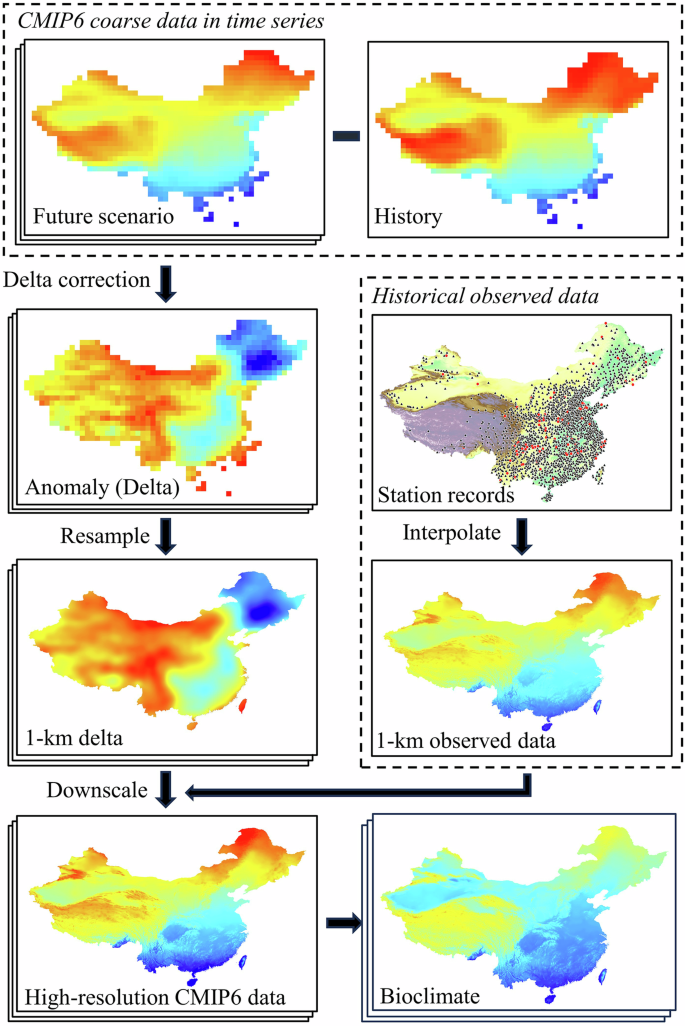
The flow chart of delta correction (DC) downscaling method.
First, we calculated the 30-year averages of tas, tasmax, tasmin, pr, and sunp for the historical simulations (1991–2014) and six future scenarios. Because the CMIP6 historical data ended in 2014, some studies, such as the CMIP6-Endorsed activity50, extended the dataset with data under SSP2-4.5, the scenario closest to reality. In this study, historical simulations during 1991–2014 were retained for subsequent calculations, as the data showed a higher correlation with observation data (1991–2020) according to pre-simulation results (Fig. S1).
Second, the monthly anomalies (i.e., delta changes) between historical simulations and future scenarios were calculated. Specifically, the anomaly was calculated as absolute difference for temperature-related variables (Eq. 1) and as relative difference for sunp (Eq. 2) and pr (Eq. 3).
where, ∆ is the delta change; T is the temperature variables including tas, tasmax, and tasmin; S is variable sunp; P is variable pr; f is the multi-year averaged climate data under future scenarios; h is the averaged historical simulations during 1991–2014; and i is each month from January to December.
Notably, the use of relative difference for pr and sunp was to avoid negative values when applying the delta change to observed data. Considering the scanty rainfall, which is even close to zero in some areas of China to result in excessively large anomaly values, two extra modifications were applied to the delta change in precipitation3,12: (1) based on the results of the prior sensitivity analysis testing a series of constants and comparison with other studies3,12, it was determined that a constant of 0.1 was added to both the historical and future data to avoid division by zero (Eq. 3); (2) the top 2% of anomaly values was truncated to the 98th percentile value in the empirical probability distribution to avoid potentially unreasonable future precipitation extremes.
Third, those monthly anomalies were resampled to the same 0.01° × 0.01° resolution as the historical observed data. The original resolutions of selected GCMs were different but unexceptionally coarse (Table 2). To obtain uniform and high-resolution data, another three commonly used resampling methods were employed including bilinear, cubic spline, and thin-plate spline, in order of calculation from simple to complex. Given the better and less time-consuming performance of the cubic spline method (Table S1), a total of 3240 resampled surfaces of monthly delta change were produced for all the GCMs, SSPs, and variables.
Finally, the downscaled future climate data were obtained by applying resampled anomalies to high-resolution historical observed data. Addition was applied to temperature variables, while multiplication was used for other variables (Eqs. 4, 5). The ensemble model was derived as the equally weighted average of the nine GCMs. The bioclimatic variables were further derived from the downscaled future basic climate variables following the aforementioned methods.
where, ∆ is the delta change; T is temperature variables including tas, tasmax, and tasmin; SP is variables including sunp and pr; Df is the downscaled future climate data; Oh is the high-resolution historical observed data during 1991–2020; I is resampled data; and i is each month from January to December.
Accuracy evaluation
The software ANUSPLIN allowed detection of errors between interpolated and observed data through generalized cross validation to evaluate interpolation accuracy. The root mean square error (RMSE; Eq. 6), mean absolute error (MAE; Eq. 7), and coefficient of determination (R2; Eq. 8) were selected as evaluation criteria in this study28. Lower RMSE and MAE values meant smaller deviation between simulated and observed data, while an R2 value close to 1 indicated a better model fit.
where, SIMi is the interpolated or simulated value at position i, OBSi the observed value at position i, and n the number of samples.
For the downscaled data, probability density functions (PDFs) were used to compare the seasonal trends of observed and downscaled data in different regions of China. PDFs could clearly illustrate the impacts of downscaling methods12. Specifically, the study area was divided into four regions (Fig. 1): Northeast (NE), Southeast (SE), Northwest (NW), and the Tibetan Plateau (TP). The annual period was further divided into four seasons, each consisting of three months: spring (March-April-May), summer (June-July-August), autumn (September-October-November), and winter (December-January-February). We selected GCM data under SSP5-8.5 in 2071–2100 to generate PDFs, as this scenario deviated the most from the current climate and thus improved the visualization. The Taylor diagram51 was also used to evaluate GCM performance more concisely. Since no future climate observation exists, some studies have chosen a period with proxy data as an independent experiment12,52. Here, we used climate data during 1951–198053 as a reference period to further analyze the downscaling methods. The observed records during 1951–1980 were derived from the same source as the baseline data during 1991–2020 to ensure the representativeness of the reference data. The GCM-simulated historical data during 1951–1980 were downscaled following the aforementioned methods. The observed and downscaled data were then compared. Additionally, the three anomaly resampling methods was also validated using the reference data.
Data Records
The dataset includes averaged monthly gridded (0.01° × 0.01°) historical data during 1991–2020 and bias-corrected future data over ten models (nine GCMs and one ensemble model), three SSPs, and three periods: 2021–2040, 2041–2070 and 2071–2100. For the history period and each future scenario, five basic climate variables were calculated including tas, tasmax, tasmin, pr, and sunp, in addition to 23 bioclimatic variables (Table 1).
All data are provided as zipped GeoTIFF (.tif) files. The file naming rules followed a consistent pattern. The historical data were named following the example China_Variable_1km_1991–2020.tif (e.g. China_pr_1km_1991–2020), where Variable is the abbreviation of 28 variables. Similarly, the future data were named following the example China_Variable_Model_VariantLabel_1km_StartYear-EndYear_Scenario.tif, (e.g. China_tasmin_MRI-ESM2-0_r1i1p1f1_1km_2071–2100_SSP585.tif), where Variable is the abbreviation of 28 variables, Model is the GCM name, VariantLabel is r1i1p1f1 as default in this study, StartYear-EndYear is the future period, and Scenario is the SSP name. For the five basic variables, tas, tasmax, tasmin, pr, and sunp, each file contained 12 layers representing 12 months in ascending order. All data are freely available at the China Science Data Bank54.
Technical Validation
ANUSPLIN performance
The ANUSPLIN outputs of historical climate during 1991–2020 showed remained similar trends to observation records in different regions (Fig. 3), with the characteristics of simultaneous rain and heat, and gradual decreases in temperature and precipitation from southeast to northwest with the distance from the ocean25,55, in contrast to the fluctuation of percentage of sunshine. Specifically, in July, the tas across China ranged from −8.50 °C to 34.26 °C, tasmax from 2.53 °C to 49.83 °C, tasmin from −22.81 °C to 26.65 °C, pr from 1.15 mm to 635.30 mm, and sunp from 19.32% to 85.14%. In contrast, in January, the tas across China ranged from −31.89 °C to 21.09 °C, tasmax from −7.99 °C to 35.28 °C, tasmin from −58.54 °C to 18.42 °C, pr from 0.38 mm to 234.96 mm, and sunp from 7.70% to 85.14%. Except for sunp, the averages of ANUSPLIN were slightly lower than those of observation records. This is caused by the sparse meteorological stations in the relatively cold and dry southwestern region of China, indicating that ANUSPLIN could modify the distribution bias of these stations11.
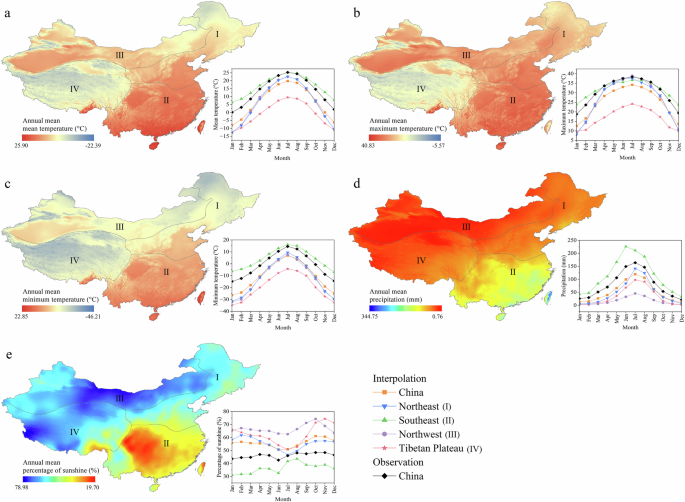
The ANUSPLIN interpolated surfaces of annual (a) mean, (b) maximum, and (c) minimum temperature, (d) annual mean precipitation, and (e) annual mean percentage of sunshine during 1991–2020. Attached curves represented the monthly trends of the interpolated results and observation records in different regions of China.
The criteria of RMSE, MAE, and R2 were commonly used to evaluate interpolation quality accurately10,11,53. Generally, the evaluation results differed due to the seasonal and regional variations in observed data but remained overall stable, indicating that the ANUSPLIN surfaces were reliable (Table 3). The RMSE in the monthly series for tas was below 0.38 °C, tasmax below 0.78 °C, tasmin below 1.45 °C, pr below 12.77 mm, and sunp below 2.57%. The MAE for tas was below 0.28 °C, tasmax below 0.54 °C, tasmin below 1.07 °C, pr below 8.14 mm, and sunp below 1.78%. Additionally, R2 for all the five variables was above 0.91. Among the five variables, the evaluation results of tas were optimal and the most stable, while the results for pr and sunp fluctuated mainly in summer. On the one hand, this may be related to the choice of covariates. The influence of elevation was more direct on temperature than precipitation and precipitation-based calculation of percentage of sunshine following the temperature lapse rate10,16. On the other hand, the interpolation for areas with higher temporal and spatial variability was sensitive to the data processing method of meteorological stations, leading to increasing difficulty in the accurate depiction of precipitation distribution11. Spatially (Table S2), the RMSE for tas was below 0.36 °C (NE), tasmax below 0.63 °C (NE), tasmin below 1.27 °C (NE), pr below 12.03 mm (SE), and sunp below 2.54% (TP). The MAE for tas was below 0.26 °C (NE), tasmax below 0.45 °C (NE), tasmin below 0.94 °C (NE), pr below 6.02 mm (SE), and sunp below 1.83% (TP). R2 for all the regions was above 0.92. Although meteorological stations were sparse in the TP, the interpolation results performed better than expected (Table S2). This also demonstrated that ANUSPLIN could remain effective in areas with sparse stations11,14.
Delta correction performance
The DC method greatly changed the regional and seasonal distribution of all basic variables (Figs. 4, 5; Figs. S2–S4). After downscaling, PDFs had similar shapes, averages and standard deviations as those of interpolated historical data. All the downscaled data successfully preserved the anomaly (i.e., delta change) between simulated historical and future data. For most regions and seasons, the distance between the PDFs of downscaled and interpolated data closely matched the gap between the historical and future GCM data. The PDFs of GCMs were mostly unimodal, while the DC method modified peak distribution and adjusted density values related to temperature frequency and precipitation intensity, such as the tas (SE) during the winter and pr (NW) during the spring, making PDF shapes closer to observations and thus improve model accuracy. For extreme variables, GCMs tended to overestimate tasmin and underestimate tasmax, which was effectively corrected by the DC method.
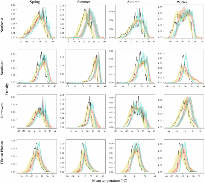
Probability density functions (PDFs) of seasonal and regional mean temperature (tas). The curves and shaded areas are the mean ± one standard deviation of PDFs derived from interpolated historical data in 1991–2020 (black), GCM historical data in 1991–2014 (yellow), GCM future data under SSP5-8.5 in 2071–2100 including original (red) and downscaled (blue) data.
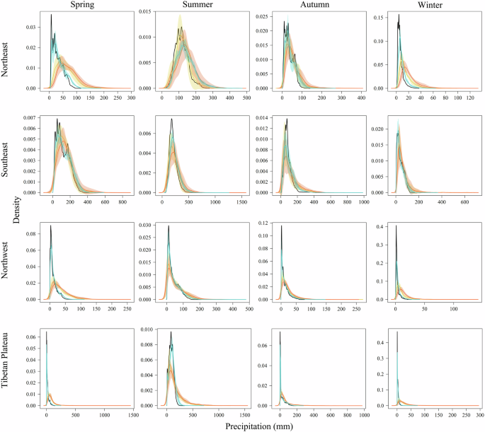
Probability density functions (PDFs) of seasonal and regional precipitation (pr). The curves and shaded areas are the mean ± one standard deviation of PDFs derived from interpolated historical data in 1991–2020 (black), GCM historical data in 1991–2014 (yellow), GCM future data under SSP5-8.5 in 2071–2100 including original (red) and downscaled (blue) data.
From the near optimistic (SSP1-2.6 in 2021–2040) to distant pessimistic (SSP5-8.5 in 2071–2100) future (Figs. 6, 7; Figs. S5–S7), all basic variables exhibited a gradually intensified increase in general, in accordance with the definition of their respective climate scenarios. The increase in average annual tas over China ranged from 0.64 °C to 5.83 °C, tasmax from 0.53 °C to 5.70 °C, and tasmin from 0.64 °C to 5.83 °C. And the change of average annual pr over China varied from −4.35% to 54.34% and sunp from −0.55% to 19.90%. Spatially, climate warming intensified from southeastern to northwestern China. Meanwhile, the increase in precipitation was concentrated in the southeast, contrary to the decrease happening in the northwest. As for sunp, its increase mainly occurred in the Tibetan Plateau.
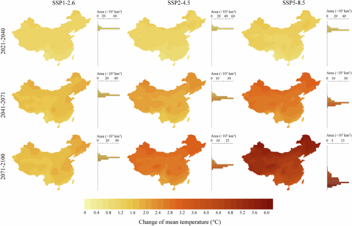
Absolute differences of future annual mean temperature minus the historical data.
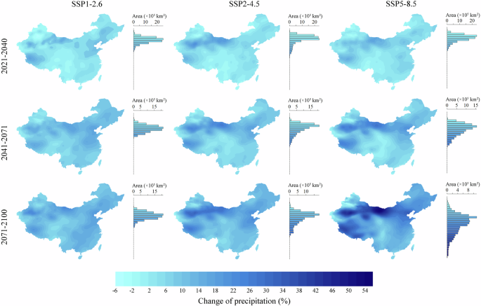
Relative differences between future annual mean precipitation and the historical data (as calculation baseline).
Similar to the evaluation of ANUSPLIN results, RMSE, MAE, and R2 were also used to validate the DC method, as recommended by many DC datasets25,28,56. The Taylor diagram was also a common tool to compare GCMs28,52,57. Additionally, we also used historical data during 1951–1980 as reference. Therefore, the evaluation of the DC method in this study was also reasonable. For reference data (Fig. 8), downscaled data had higher fitness with historical observations. The average RMSE of downscaled data across nine GCMs for tas, tasmin, pr, and sunp reduced by 58.63%, 0.69%, 53.35%, and 58.44%, respectively. The average correlation coefficient increased by 3.51%, 2.13%, 26.32%, and 71.35%, respectively. However, for tasmax, the average of RMSE increased by 7.96% and the average of correlation coefficient decreased by 1.56%. Overall, all correlation coefficients were above 0.92 after downscaling, indicating that the DC method could improve the resolution and accuracy of CMIP6 data. Among the basic variables, the downscaling results of temperature performed better (Fig. 8). Usually, the downscaling of temperature was more operable28, partly because of the inherently greater divergence among different GCMs for original precipitation data than temperature (Fig. 8; Fig. 9). Also, it was more constrained to fully explain precipitation, like the bias of AUSPLIN results abovementioned (Table 3). Among the nine GCMs, the models that performed the best for tas, tasmax, tasmin, pr, and sunp before downscaling were CMCC-ESM2, GFDL-ESM4, MPI-ESM1.2-HR, MPI-ESM1.2-HR, MIROC6. After downscaling, the better models were BCC-CSM2-MR, MIROC6, BCC-CSM2-MR, INM-CM5.0, MIROC6, respectively. Among GCMs, downscaled data presented higher stability in the average and variance (Fig. 9).
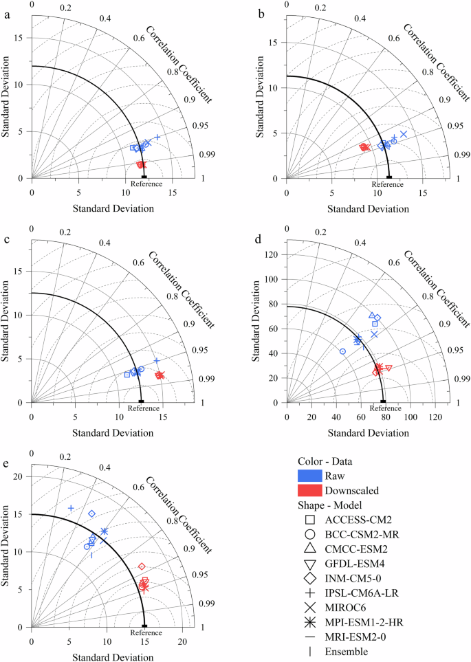
Taylor diagrams based on the outputs of DC downscaled results of five basic variables. a. tas; b. tasmax; c. tasmin; d. pr; e. sunp.
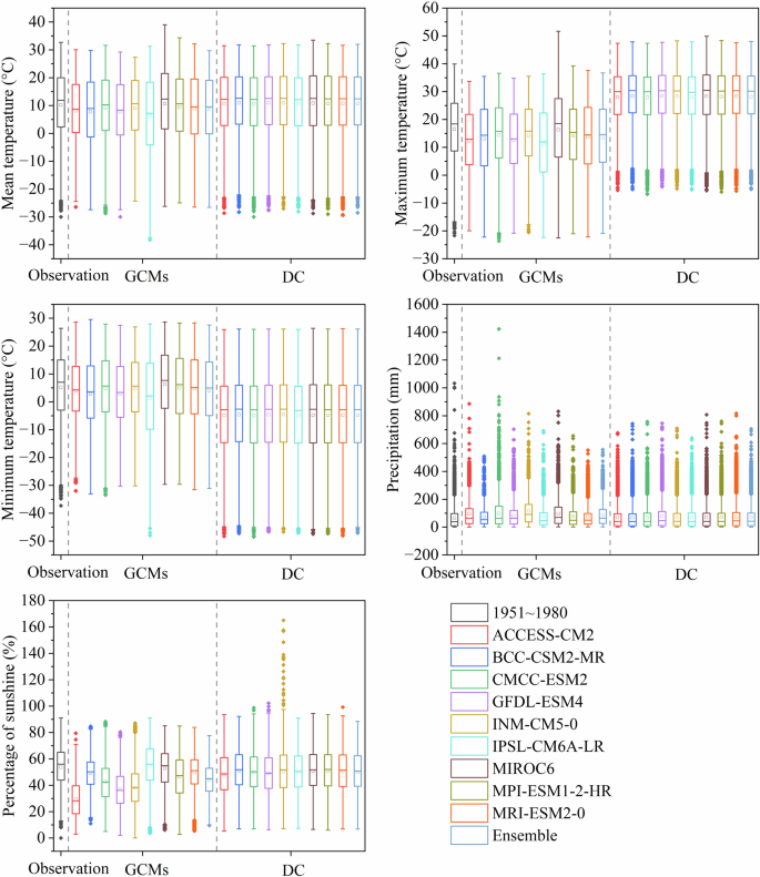
Boxplots based on five basic variables from observation records, original GCM outputs, and downscaled GCM outputs.
Additionally, note that bias correction could not calibrate fundamentally a GCM performing poorly26, such as the INM-CM5-0 model for sunp projections (Fig. 8). In this case, the ensemble model was a solution to further correct biases among GCMs27. In this study, we used the arithmetic mean of GCMs as an example. The ensemble model further promoted the performance of DC method. After downscaling, the RMSE for tas, tasmax, tasmin, pr, and sunp decreased by 3.82%, 0.56%, 0.62%, 11.68%, and 19.73%, and the correlation coefficient increased by 0.06%, 0.12%, 0.04%, 1.25%, and 2.62%, respectively. The ensemble model performed better than each GCM for tas, pr, and sunp, and preceded only by the optimal model abovementioned for the rest variables. The ensemble method used here was the simplest approach, and users could further calculate customized ensemble models to satisfy their own demands.
Comparison with previous studies and other products
To compare our dataset with other climate products and previous studies, we extracted monthly averaged data for 1991–2020 from other datasets (Table S3) and analyzed the relationships between these datasets and meteorological records (Table S4). The results showed that our dataset provided more variables which exhibited a better fit with the meteorological records than other datasets. Overall, the gridded climate data interpolated based on station records performed better than those based on multi-source and reanalyzed climate products2, especially for the extreme variables and percentage of sunshine (Table S4). Among these datasets, our dataset was established based on more meteorological stations. This probably also resulted in its higher accuracy. In the future, the overall projections would increase all the five basic climate variables in most areas. Similar trends and spatial patterns were also observed in previous predictions based on CMIP6 data58,59,60,61. For example, it was predicted that the increase in precipitation would reach 57.44% at most in the northwestern China in the 2090 s under SSP5-8.561, which was similar to the above 50% future increase occurring in the same region in this study (Fig. 7). However, these datasets differed in values due to the choices of scenarios and GCMs. Therefore, further uncertainty analysis is necessary to determine the suitability of data under different situations before application.
Uncertainty
As validated in this study, ANUSPLIN demonstrated good interpolation performance, by accounting for spatial variations such as elevation and relying on all observed data for modeling, even in data sparse, high-elevation regions62. However, it was difficult to fully explain local conditions in areas with complex climate depending on only the interpolation software, particularly for microclimate phenomena such as temperature inversions62,63. In this case, the most effective solution was supplementing local observation records, and it could also enhance interpolation accuracy by incorporating climate information from neighboring areas17. Therefore, to enhance the accuracy of ANUSPLIN outputs, the improvement of data sources was also a feasible choice.
Compared with CMIP5, CMIP6 data have improved simulations of temperature and precipitation, particularly for climate extremes64. However, the downscaling results of the two extreme variables tasmax and tasmin were still partly biased. Compared with the observed average, the median of downscaled tasmax increased by about 11 °C, while the downscaled average of tasmin decreased by about 10 °C (Fig. 9). The prediction of extreme events tended to be uncertain. Although correct changing trends could be retained by DC65, some studies showed underestimation of minimum and overestimation of maximum when applying DC method, which was possibly caused by relatively higher sensitivity of extreme variables to the choice of GCMs and downscaling techniques, as well as fluctuation of climate changing signals in data processing26,52,66,67. This may be the reason why the improvement in the two extreme variables, tasmax in particular, after downscaling was not as obvious as that of other variables. However, considering that the evaluation results of the basic climate variables were close to each other and confident statistically, and that the influences of extreme variables were inevitably partly eliminated after 30-year averaged data processing12, we believed that the data were reliable and they should be used more cautiously when analyzing the impacts of extreme temperature on defined period and location.
Except the variable differences, the methods of anomaly resampling could also play a part in the DC performance. The methods used in this study included bilinear, cubic spline, and thin-plate spline, which were all commonly used and helped promote DC accuracy3,12,25. The final choice of cubic spline was based on its slight advantage in statistical analysis, while the differences among the three methods were minimal (Table S1). This is because, as least in this study, the resampling method was not the main factor for DC. Additionally, the DC performance exhibited spatial variability during the same period, which may be influenced by the accuracy of the baseline data25,26. For instance, three covariates were introduced in the WorldClim dataset, including elevation, distance to the coast and three satellite-derived covariates, to improve data accuracy20. On this basis, the DC downscaled data had also better accuracy25. In this study, the baseline data of interpolated grid during 1991–2020 incorporated abundant stations and their records from official source, thus ensuring the accuracy of downscaled future data.
Usage Notes
Based on ANUSPLIN software and DC downscaling method, our dataset contained five basic climate variables and 23 bioclimatic variables. Each variable covered the historical period and six future climate scenarios, and thus had a wide range of applicability. Firstly, these variables could be used to study the relationships between climate and species, populations, communities, and ecosystems. Data from multiple periods of each variable could also be used to study the impact of climate change on species distribution, ecosystem patterns and functions. Secondly, considering the current data storage costs, we provide only 28 commonly used variables. However, this did not mean that these data were limited to the variables. Instead, users could still further calculate other customized variables such as actual evapotranspiration and the plant-available moisture index38,68 based on the dataset. Thirdly, as emphasized above, regardless of the dataset used, users should consider the potential biases and determine whether these biases would affect their research. Specifically, the long-term averaged monthly climate data we provided in this study should be applied more carefully when analyzing extreme climate change and annual variation. In the future, more observation data will be collected, as this remains the most effective and direct method to improve data accuracy. Moreover, with the continuous progress of GCMs, we also believe that GCM outputs will achieve higher precision and accuracy, thereby providing better climate data for various fields.


Responses