A computational spectrometer for the visible, near, and mid-infrared enabled by a single-spinning film encoder

Spectrometers are essential instruments for analyzing the spectral composition of light, providing critical information in the fields of chemistry¹, biology², environmental science³, and remote sensing⁴. In traditional designs, broadband light is divided using dispersive optical components, e.g., gratings, prisms, and optical filters, before being captured by a photodetector. These dispersive optics are particularly effective for the visible and near-infrared wavelength range, providing ultra-high spectral resolution. In contrast, the Fourier Transform Infrared (FTIR) spectrometers are commonly used for mid- and far-infrared spectral analysis. FTIR spectrometers utilize an interferometer to modulate the light and produce an interference pattern, which is then mathematically transformed into a spectrum. This method allows for the simultaneous measurement of all wavelengths, offering high sensitivity and rapid data acquisition. However, both traditional dispersive spectrometers and FTIR systems are often hindered by the benchtop size and high production costs, limiting the applications where low-cost, miniaturization and in situ analysis are prioritized over high spectral performances.

Over the past decade, computational spectrometers have gradually emerged as a promising alternative. Compared with commercial spectrometers based on dispersive elements or interferometers, computational spectrometers still face inherent challenges in balancing spectral accuracy and working bandwidth. Moreover, the adaptability to varying environmental conditions, e.g., variations in the angle of light incidence, remains limited, further hindering their broader commercialization. Nevertheless, these ultra-compact, cost-effective, and low-power devices hold potential in highly integrated systems, e.g., portable or wearable devices and unmanned aerial vehicles (UAVs). Recent advancements in micro- and nano-fabrication, coupled with the development of compressive sensing and artificial intelligence algorithms^5,6,7,8,9, propelled the evolution of computational spectrometers.

For the aspect of spectral encoding, the strategies can be categorized into two main approaches, one based on filters with broad responses atop detectors and the other on detector-only configurations. For filter-based encoding strategy, optical elements capable of exhibiting diverse spectral responses are potential candidates for spectral encoders. Notable examples include quantum dots^10,11,12,13, thin films^{14,15,16,17,18}, photonic crystal slabs^19,20, and metasurfaces^21,22,23,24. Filters are commonly configured as arrays, facilitating rapid spectral encoding in a single-shot manner, which is beneficial for real-time applications. Detector-only configurations rely on the inherent spectral sensitivity of the detectors themselves, which can be achieved through material engineering and the integration of nanostructures. These configurations can be divided into schemes employing single-dot detectors^{25,26,27,28,29,30,31} and detector arrays^32,33. In the case of single-dot detectors, distinct spectral responses are typically generated by applying varying bias voltages, and such a method indicates the ultimate miniaturization of computational spectrometers. However, it also has drawbacks. Typically, a given material responds to a limited spectral band, which constrains the applicability across broader wavelengths. The responsivity of the detector may be unstable, particularly under fluctuating temperature and humidity conditions, which limits the long-term reliability of the spectrometer. In the case of detector array-based spectral encoding, reported works are limited due to the high fabrication complexity and relatively low yield rates.

Afterward, the unknown spectrum is recovered using the reconstruction network from the compressed measurements. Commonly, the number of spectral encoders is fewer than the discrete wavelength channels, which indicates an underdetermined problem. To address the resulting ill-posed equations, compressive sensing-based reconstruction algorithms are initially employed^10,32,34,35. Such an iterative method benefits from advanced anti-noise capabilities. However, the reconstruction speed is relatively slow, especially in spectral imaging applications. In contrast, deep learning, characterized by its data-driven approach and high-speed processing, is increasingly applied for spectral reconstruction^{11,16,22,29,36,37,38,39,40}. It leverages the substantial computational power of graphics processing units (GPUs) to efficiently reconstruct complex spectral information, rendering it highly suitable for real-time applications. However, deep learning-based reconstruction networks are more sensitive to noise compared to compressive sensing-based networks. To address this limitation, many studies introduce additional noise, such as Gaussian white noise, to enhance the robustness of neural networks during the training process. Furthermore, the diversity of the training dataset is often expanded to improve the generalization capability of the network.

In comparison, the filter-based computational spectrometer is more stable and technically mature, holding greater commercial potential. However, it often necessitates micro- and nano-fabrication solutions for array construction, e.g., photolithography, electron beam lithography, and etching, resulting in increased manufacturing costs and more complex fabrication processes. Additionally, the spectral responses between different devices may vary due to the muti-step manufacturing approaches. Furthermore, spectral encoders that are applicable across multiple wavelength bands have rarely been reported. As shown in Supplementary Table 1, the majority of prior works are focused on a single spectral band, such as the visible wavelength range.

Addressing these issues, we advance ultra-broadband spectral encoding by leveraging the inherent characteristics of an individual filter, rather than relying on the cross-correlation between different encoding elements. In this work, we harness the polarization separation effect under oblique incidence (PSEOI) and employ the single-spinning film encoder (SSFE) with broadband spectral responses spanning the visible (400–700 nm), near-infrared (700-1600 nm), and mid-infrared (3-5 μm) wavelength ranges for highly efficient spectral encoding. This represents one of the few attempts to perform multi-wavelength spectral computation using a well-defined encoding device. The thickness of each layer is predesigned using the particle swarm optimization (PSO) method to achieve specific spectral response requirements, e.g., minimal spectral correlation and enhanced spectral complexity. SSFE is fabricated using a one-step electron beam evaporation (EBE) process, enabling large-area fabrication and repeatable manufacturing. Utilizing the deep learning-based reconstruction algorithm, spectral reconstruction can be performed at a higher speed compared to traditional iterative methods. The high spectral resolution is achieved across the visible, near-infrared, and mid-infrared wavelength bands, recorded as 0.5 nm, 2 nm, and 10 nm for single-peak spectra across these bands, respectively, and 3 nm, 6 nm, and 20 nm for dual-peak spectra. Additionally, the overall effectiveness for classifying chemical compounds within the mid-infrared wavelength range has been verified, highlighting its potential for advanced analytical techniques in both scientific and industrial fields.

Framework of the computational spectrometer with single-spinning film encoder and deep learning

The schematic diagram of the proposed computational spectrometer is shown in Fig. 1a, with the polarizer, SSFE, and detector arranged sequentially. In the optical setup in Fig. 1a, the absolute transmittance of the sample can be reconstructed, regardless of the spectrum of the illumination. On the other hand, for spectral resolution tests, the broadband light source is used in conjunction with a monochromator to generate narrowband spectra with varying center wavelengths and linewidths, as shown in Supplementary Fig. 1, where the sample is omitted. To achieve single-filter-based spectral encoding, we take advantage of PSEOI by utilizing SSFE and a polarizer. The polarizer facilitates the generation of two separate spectral responses, R_p and R_s, by dividing the light into P– and S-polarizations, thereby doubling the number of spectral responses R. High and low refractive index materials (TiO₂ and SiO₂) are deposited alternatively on a visible to mid-infrared transparent sapphire substrate to form the 10-layer compact film stack, as shown in Fig. 1b. By progressively spinning SSFE from 0° to a maximum value of 70°, as depicted in Fig. 1c, a dynamic variation in spectral responses is observed. The gradual rotation alters the light filtering properties of SSFE, resulting in angle-dependent spectral encoding.

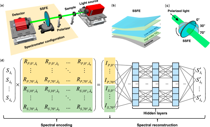
a The optical setup of the system, with a broadband light source, sample, and the SSFE-based spectrometer, including a polarizer, SSFE, and detector arranged sequentially. b Structure of the 10-layer SSFE composed of alternating high-index TiO₂ and low-index SiO₂ on a sapphire substrate. c Diagram illustrating the rotation of SSFE, with a rotational angle ranging from 0° to a maximum value of 70°. Specifically, the rotation angles for P-polarized light are 0°, 10°, 20°, 25°, 30°, 35°, 40°, 55°, 50°, 55°, 60°, 65°, and 70°, while the rotation angles for S-polarized light are 10°, 20°, 25°, 30°, 35°, 40°, 55°, 50°, 55°, 60°, 65°, and 70°. d Workflow of the spectral encoding and reconstruction procedure. Herein, spectral encoding is accomplished by SSFE, and the sensing matrix R is composed of the transmittance of SSFE under different polarizations and spinning angles. Spectral reconstruction is achieved using a deep learning-based reconstruction network featuring fully-connected layers, where the input layer corresponds to the measured light intensities I_i, the output layer represents the reconstructed spectra, and the three hidden layers are employed to capture the complex spectral relationships and enable accurate reconstruction.

Full size image

Workflow of the spectral encoding and reconstruction procedure is shown in Fig. 1d. For spectral encoding, the intensity vector collected by the detector ({({I}_{P, {0 ^{circ}} },{…},{I}_{P, {70 ^{circ}} } ,,{I}_{S,{0 ^{circ}} },, {..}.,{I}_{S, {70 ^ {circ}} })}^{{{rm{T}}}}) of an unknown spectrum (S(lambda )) propagating through SSFE can be expressed as

By discretizing the spectral dimensions, Eq. (1) can be rewritten as

where R is the precalibrated sensing matrix. Here, the number of rows in R corresponds to distinct rotation angle combinations, while the number of columns corresponds to the discrete spectral channels.

Subsequently, deep learning is employed for efficient spectral reconstruction. The entire neural network consists of a fixed encoding network and a trainable reconstruction network, as shown in Supplementary Fig. 2. The settings of the training/validating datasets are provided in Method. During the training of the entire neural network, spectral encoding by SSFE is substituted by the fixed encoding network, structured as an unbiased fully connected layer. The fixed weight matrix represents the precalibrated sensing matrix R. By comparing the reconstructed spectra ({{rm{S}}}^{prime}) with the reference spectra S in the training/validating dataset, the end-to-end neural network is optimized by solving

where (W,,theta) are the parameters (weights and biases) of the trainable reconstruction network D. For spectral reconstruction, the entire neural network is truncated, and I_i serves as the input of the trainable neural network.

Design of the single-spinning film encoder

Reconstructing the unknown spectrum involves solving the underdetermined Eq. (2), thereby necessitating the application of compressive sensing theory in general. Accordingly, the sensing matrix R needs to exhibit a certain level of randomness, i.e., the low correlation of the spectral responses, to ensure stable reconstruction in principle. Based on previous related works, we identify and extract two key factors for designing the SSFE: (1) low correlation coefficient, and (2) high spectral complexity of the spectral responses under different polarizations and spinning angles. Herein, a low correlation coefficient contributes to more independent information in the spectral responses, which helps avoid redundancy in spectral encoding and ensures that each measurement provides unique data for the reconstruction process. High spectral complexity, on the other hand, ensures that the spectral responses contain more detailed information. Multiple peaks and valleys enable the extraction of information for various wavelengths, providing a richer set of features for precise spectral reconstruction.

We employ the particle swarm optimization (PSO) method to design the structure of SSFE, capitalizing on the efficiency in convergence and simplicity in implementation^41,42. Moreover, the PSO method excels in quickly reaching global optimal solutions without getting trapped in local minima, making it ideal for straightforward optimization tasks. The layer number is predetermined to be 10, with a predefined upper limit for the thickness of each individual layer. The spectral responses, R_p and R_s, corresponding to the specific layer thickness, are determined using the transfer matrix method⁴³. These responses are then employed to calculate the Figure of Merit (FoM). Specifically, during the optimization process, FoM serves as the guiding metric, and the spectral responses are optimized for minimal correlation and enhanced complexity. Taken as an example, the FoM for the visible wavelength range can be expressed as

where ({bar{r}}_{Vis}) represents the average value of the correlation coefficients ({r}_{ij}), and ({bar{V}}_{Vis}) indicates the internal differences of the spectral responses({V}_{i}). The detailed description of ({bar{r}}_{Vis}) and ({bar{V}}_{Vis}) are shown in Supplementary Note 1. A and B are the weighting coefficients that balance the importance of ({bar{r}}_{Vis}) and ({bar{V}}_{Vis}) during the optimization process, specifically set as 20 and 1, respectively. The comparison of different weight selections for A and B is presented in Supplementary Fig. 3.

The evaluation functions for near and mid-infrared (FoM_NIR and FoM_MIR) follow the same formulation as in Eq. (4). Spectral responses across the visible, near, and mid-infrared wavelength ranges are optimized simultaneously, to obtain high encoding efficiency and consequently excellent spectral reconstruction performance across the ultra-broadband wavelength ranges. Therefore, the overall FoM can be expressed as

The comparison of different weight selections for FoM_Vis, FoM_NIR, and FoM_MIR is presented in Supplementary Fig. 4. The detailed description and settings for the PSO method are outlined in Supplementary Note 2. Optimization for the varying maximum thicknesses of each individual layer, ranging from 250 nm to 1500 nm, is conducted, generating a variety of film configurations. Figure 2a showcases the evolution of GBest, i.e., the most optimal FoM achieved by the entire swarm, for these varying thicknesses during the optimization procedure. In this case, a lower GBest indicates a lower correlation and higher spectral complexity of R_i. The PSO method represents an intuitive method for optimizing the film configuration of SSFE from the perspective of spectral response characteristics. Furthermore, it is crucial to assess the efficacy of these optimized film configurations through reconstruction performances, as it offers a more direct and tangible evaluation.

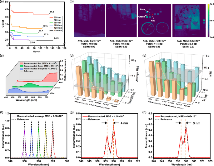
a Variations of GBest during the iteration process with different maximum thicknesses of each layer within SSFE. The optimization automatically stops when GBest remains unchanged for 50 consecutive iterations. b The error maps for reconstructing the HSIs in CAVE and ICVL using the optimized film configuration with an upper thickness limit of 1000 nm. Evaluation metrics, e.g., MSE, PSNR and SSIM, are calculated for each HSI. c The reconstructed and reference spectra of the RGB patches in Fig. 2b, the MSEs are 9.1×10^-5, 5.7 × 10^-5, and 7.8 × 10^-5, respectively. d Relationship between the average MSEs and maximum thickness of each individual layer for reconstructing the single-peak narrowband spectra with 1.5 nm, 1.0 nm, and 0.5 nm linewidths. The gray plane indicating accurate spectral reconstruction is set as 5.0 × 10^-4. e Relationship between the average MSEs and maximum thickness of each individual layer for reconstructing the dual-peak narrowband spectra with peaks spaced 4.0 nm, 3.0 nm, and 2.0 nm apart. The gray plane indicating accurate spectral reconstruction is set as 5.0 × 10⁻⁵. f Reconstruction of single-peak narrowband spectra with 0.5 nm linewidth. The average MSE is 2.86 × 10^-4. g, h Reconstruction of dual-peak narrowband spectra with peaks spaced 4 nm and 3 nm apart. The MSEs are 4.10 × 10^-5 and 4.66 × 10^-5, respectively.

Full size image

Subsequently, numerical simulations are performed, aiming to find the optimal balance between minimizing the total film thickness, i.e., reducing deposition time and manufacturing costs, while simultaneously achieving prominent performance across ultra-broadband wavelengths. The comprehensive assessment involves reconstructing broadband, single-/dual-peak narrowband spectra. For broadband spectral reconstruction in the visible wavelength range, simulations are conducted using the hyperspectral image (HSI) datasets CAVE⁴⁴ and ICVL⁴⁵. The number of spectral channels in CAVE and ICVL is expanded to 301 through linear interpolation within 400 nm to 700 nm wavelength range with 1 nm spacing. To evaluate the reconstruction accuracy, mean square error (MSE), peak signal-to-noise ratio (PSNR), and average structural similarity (SSIM) for all spectral channels are set as key evaluation metrics. Detailed descriptions of these metrics are presented in Supplementary Note 3. The error maps showcasing the MSE of each pixel in the HSIs of the upper limit of 1000 nm are shown in Fig. 2b, with results for other thickness upper limits provided in Supplementary Fig. 5. With the thickness of each layer limited to 1000 nm, the PSNR exceeds 35 dB and the SSIM consistently surpasses 0.97, indicating a high level of precision for spectral reconstruction of broadband spectra. In Fig. 2c, we display the reconstructed and the reference spectra of the RGB patches in Fig. 2b. Remarkably, the average MSE is maintained within the 10^-5 magnitude, demonstrating exceptional reconstruction accuracy. Additionally, single-/dual-peak narrowband spectra are also reconstructed. The variations in the average MSE with different thickness upper limits are depicted in Fig. 2d, e. The gray planes within these figures indicate levels at which accurate spectral reconstruction is achieved, with values of 5.0 × 10^-4/5.0 × 10^-5 for single-/dual-peak narrowband spectra reconstruction, respectively. It is observed that the average MSE generally decreases as the maximum thickness increases, demonstrating an overall trend towards improved spectral accuracy with thicker film layers. However, as the maximum thickness increases, the reconstruction accuracy may deteriorate, as shown in Fig. 2e. In such circumstance, highly complex spectral responses are regarded as white noise, which disrupts the clear correlation between I_i and the unknown spectra during the spectral encoding process. Moreover, the maximum thickness of 1000 nm is already sufficient to achieve precise reconstruction of single-peak spectra with a linewidth of 0.5 nm, as well as dual-peak spectra with peaks spaced 3 nm apart, as shown in Fig. 2f–h and Supplementary Fig. 6, consistent with that observed at greater maximum thicknesses. More comparisons in the near and mid-infrared wavelength ranges are provided in Supplementary Fig. 7. It is noted that maximum thicknesses below 1000 nm substantially reduce the dual-peak resolution in the mid-infrared wavelength range. Numerical tests for near and mid-infrared wavelength range with a maximum thickness of 1000 nm are detailed in Supplementary Fig. 8 and Supplementary Fig. 9. Based on the aforementioned comprehensive performance evaluation and comparison, an optimized encoder configuration with a maximum thickness limit of 1000 nm is selected.

Fabrication and characterization of the single-spinning film encoder

Based on the preceding analysis, the thickness limit of each individual layer during the optimization procedure is set as 1000 nm. The optimized thickness distribution for the 10-layer SSFE is depicted in Fig. 3a, with a total thickness of 7393 nm. Particularly, the thicknesses for the TiO₂ and SiO₂ layers are 4097 nm and 3296 nm, respectively. The SSFE is fabricated with one-step electron beam evaporation (EBE) process, specifically selected to bypass micro- and nano-fabrication, thereby reducing the manufacturing complexity and cost. The deposition rates for TiO₂ and SiO₂ are 0.5 nm per second and 0.8 nm per second, respectively, and the entire deposition process totaling about 3.5 h. Due to the exclusive application of the mature thin film deposition technique, the optical performance of SSFE is highly consistent and repeatable, eliminating the need for retesting the spectral responses and retraining of the reconstruction network. Following this, angle-dependent spectral responses are measured under different polarization states using both spectrophotometer (for visible and near-infrared) and FTIR (for mid-infrared), shown in Fig. 3b and Supplementary Fig. 10. On the 4-inch-diameter SSFE, the uniformity is evaluated by measuring the transmittance across several distinct positions, shown in Fig. 3c. Low correlation coefficients of the spectral responses in the visible wavelength range can be obtained with an average value of 0.19, as shown in Fig. 3d. By simply spinning SSFE, the spectral responses at adjacent angles, e.g., R_p,0° and R_p,10° (the correlation coefficient is 0.95), or R_p,40° and R_p,45° (the correlation coefficient is 0.53) exhibit relatively high similarity. In addition, the correlation between R_p and R_s is more pronounced at smaller angles, e.g., R_p,20° and R_s,20° (the correlation coefficient is 0.96). Accordingly, measurements are taken at 10° intervals at smaller angles (0°, 10°, and 20°), and reduced to 5° intervals for larger angles (20°, 25°,…, 70°). The correlation coefficients of the spectral responses in near and mid-infrared are shown in Supplementary Fig. 11, with average values of 0.24 and 0.44, respectively. For the same physical thickness, an increase in wavelength leads to larger spacing between adjacent spectral peaks or valleys, as explained by thin-film interference theory, and also vividly illustrated in the spectral responses of different wavelength ranges in Fig. 3(b) and Supplementary Fig. 10. This results in simpler spectral responses and lower correlation, as detailed in Supplementary Note 4. Consequently, spectral reconstruction in longer wavebands, such as the near and mid-infrared wavebands, presents greater challenges compared to that in shorter wavelengths.

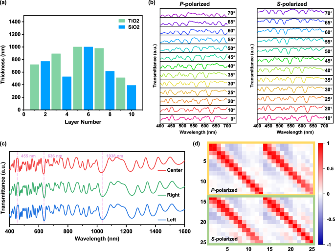
a The optimized thickness distribution of the 10-layer SSFE. The first layer is near the substrate side. The total thickness is 7393 nm, and the thicknesses for the TiO₂ and SiO₂ layers are 4097 nm and 3296 nm, respectively. b Measured angle-dependent spectral responses under different polarization states in the visible wavelength range. The complex spectral response, characterized by various peaks and valleys, contributes to low correlation, which supports efficient encoding. c Measured transmittance across several distinct positions on the 4-inch-diameter SSFE in the visible and near-infrared wavelength range. The dashed lines serve as references to highlight the consistency of peak/valley wavelengths. d Correlation coefficients of the spectral responses in the visible wavelength range. A remarkably low average correlation of 0.19 is achieved.

Full size image

Spectral reconstruction in visible, near, and mid-infrared wavelength ranges

In practical scenarios, system and measurement noise affect reconstruction accuracy. Therefore, we introduce additional noise to simulate actual experimental conditions during neural network training. This approach helps the network avoid overfitting to noise-free or specific training data, ensuring greater robustness and improved reconstruction performance. Equation (3) can be rewritten as

where (sigma) refers to the noise level, which typically varies with different types of detectors and testing environments, and (e) follows the standard normal distribution. To examine the spectral resolution in the visible wavelength range, we reconstruct the single-peak narrowband spectra with center wavelengths ranging from 500 nm to 600 nm with 10 nm spacing, as shown in Fig. 4a. The average MSE is 1.05×10^-3, and the average center-wavelength error and linewidth error are recorded as 0.61 nm and 0.56 nm, respectively, as detailed in Fig. 4b and Fig. 4c. Figure 4d–f displays spectral reconstruction results of the absolute transmittance for color filters. The red/blue solid lines represent the reconstructed spectra using the experimental/calculated intensities. Detailed descriptions of these two intensities are provided in Supplementary Note 5. By introducing an ideal reconstructed spectrum, we can find that the reconstruction errors stem from both system inaccuracies (by comparing the reconstructed spectra using the experimental and calculated intensities) and the limited generalizability of the neural network (by comparing the reference spectra and the reconstructed spectra using the calculated intensities). The average MSEs are 4.69 × 10^–3 and 8.87 × 10^-4 using the experimental/calculated intensities. For reconstruction of near-infrared spectra, we numerically reconstruct the transmittance of diverse filters with different spectral distribution, shown in Fig. 4g–i, demonstrating high accuracy with an average MSE of 3.82 × 10^-3. Moreover, in the mid-infrared wavelength range of 3-5 μm, we experimentally reconstruct two broadband spectra generated by a broadband halogen lamp and altering filters, shown in Fig. 4j, k. The average MSE drops to 5.30 × 10^-3, lower than that observed in the visible wavelength range. The primary reason for the performance decline is the application of the uncooled infrared detector, which generates substantial noise and results in a relatively large spectral reconstruction error. To examine the spectral resolution in mid-infrared wavelength range, narrowband spectra with 10 nm linewidths are successfully reconstructed, shown in Fig. 4l. Herein, the average MSE is 3.36 × 10^-4. In the future, several methods can be explored to improve the overall performance of mid-infrared spectral reconstruction, including the application of cooled detectors to reduce noise levels, adaptive noise filtering techniques, e.g., Wiener filter or Kalman filter, and modified training strategies for the reconstruction network, e.g., training the network using datasets acquired from the actual detector, to enhance its accuracy under noisy conditions.

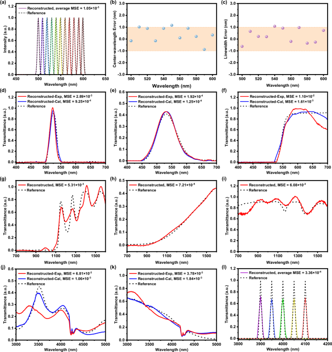
a Reconstruction of narrowband spectra in the visible wavelength range (400 nm to 700 nm with 1 nm spectral channel spacing). The center-wavelength ranges from 500 nm to 600 nm with 10 nm spacing. The black dashed lines represent the reference spectra measured by a commercial spectrometer, while the colored solid lines are the reconstructed spectra. The average MSE is 1.05 × 10^-3. b, c The center-wavelength error and linewidth error distributions for narrowband spectra reconstruction. The average errors are 0.61 nm and 0.56 nm, respectively. d–f Reconstruction of broadband spectra. The broadband spectra are the absolute transmittance of color filters. The black dashed lines represent the reference spectra measured by a spectrophotometer, and the red/blue solid lines are the reconstructed spectra using experimental/ calculated intensities. The MSEs are 2.89 × 10^-3, 1.92 × 10⁻⁴, and 1.10 × 10^-2 using the experimental intensities, whereas the MSEs decrease to 9.25 × 10^-3, 1.25 × 10⁻⁴, and 1.61 × 10^-3 using the calculated intensities. g–i Simulative reconstruction of broadband spectra in the near-infrared wavelength range (700 nm to 1600 nm with 3 nm spectral channel spacing). The black dashed lines represent the reference spectra, while the red solid lines are the reconstructed spectra. The MSEs are 5.31 × 10^-3, 7.21 × 10⁻⁵, and 6.08 × 10^-3, respectively. j–k Reconstruction of broadband spectra in the mid-infrared wavelength range (3 μm to 5 μm with 5 nm spectral channel spacing). The MSEs are 6.81 × 10^-3 and 3.78 × 10^-3 using the experimental intensities, whereas the MSEs decrease to 1.06 × 10^-3 and 1.84 × 10^-3 using the calculated intensities. l Simulative reconstruction of narrowband spectra with 10 nm linewidths. The average MSE is 3.36 × 10⁻⁴.

Full size image

Application in chemical compound classification in mid-infrared wavelength region

To demonstrate the potential application of the SSFE-based computational spectrometer, we conduct numerical tests to showcase the efficacy of chemical compound classification in the mid-infrared wavelength region. The transmittance of 220 commonly-used liquid chemical compounds in the laboratory constitutes the training/testing dataset (obtained from NIST)⁴⁶. Notably, the dataset is further expanded by introducing spectral variations to simulate different purities and concentrations of the chemical compounds. Figure 5a shows the accurate spectral reconstruction of several chemical compounds with an average MSE of 1.21 × 10^-3, demonstrating the potential for reliable chemical analysis and identification. The predicted label of the chemical compounds is determined by comparing the reconstructed spectra with the reference spectra in the dataset. For the chemicals in Fig. 5a, the system correctly identifies the labels, i.e., the types of chemical compounds. However, classification errors do occur, shown in Supplementary Fig. 12. It is observed that the MSEs of the misclassifications are not lower than those of correct classifications in Fig. 5a. The misclassifications primarily stem from the similarity of the spectral profiles among the chemical compounds. To further investigate this, we conduct 5000 tests, and among the 872 misclassifications, the relative differences (D) between the reference spectra of the true labels and the corresponding false labels are calculated by

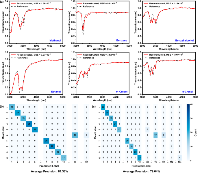
a Reconstruction of the transmittance of chemical compounds. The black dashed lines represent the reference spectra, while the red solid lines are the reconstructed spectra. The average MSE is 1.21 × 10⁻³. b–c Confusion matrix of the classification results for the first 10 out of the overall 220 chemicals in the dataset with the noise level of (b) 0.025 and (c) 0.05. At the noise level (sigma) of 0.025 and 0.05, the average precisions for all chemicals are 81.38% and 79.04%, respectively, across 5000 tests.

Full size image

Here, S_i1 represents the reference spectra of the true label, while S_i2 denotes the reference spectra of the false label. The average D is recorded as 3.59%, as shown in Supplementary Fig. 13, with 97.7% of the misclassifications (852 out of the 872) occurring when D is below 6.5%. These results suggest that when the spectral profiles of two chemical substances exhibit high similarity, the likelihood of misclassification increases. Additionally, the transmittance spectra of chemical compounds in mid-infrared often feature notch-shaped characteristics. Compared to the bandpass spectra with peaks at specific wavelengths, spectral reconstruction and classification become more challenging.

Similarly, we introduce varying levels of noise to the testing dataset to address the measurement and system errors, and to evaluate the robustness of classification. When no noise is added, the average precision is 81.68% for 5000 tests. With a noise level (sigma) of 0.025, the average precision is 81.38%. The confusion matrix of the first 10 chemicals out of the 220 chemicals in the dataset is shown in Fig. 5b. By enhancing the noise level (sigma) to 0.05, the average precision drops down to 79.04%, as depicted in Fig. 5c. Among the 10 compounds, the number of chemicals with identification errors increased from 1 (chemical 6) to 4 (chemicals 5, 6, 8, 10). The trend between the noise level (sigma) and the average precision is illustrated in Supplementary Fig. 14. It can be observed that under a noise level of 0.1, the identification accuracy can still be maintained at a relatively high standard, exceeding 70%, demonstrating the system’s robustness and stability. A comparison of our work with the existing chemical compound classification devices and technologies is presented in Supplementary Table 2.

Comparison of SSFE-based computational spectrometer with the existing designs

A detailed comparison of our work with some previously reported computational spectrometers is presented in Supplementary Table 1, including the comparisons of the encoder type, wavelength range, number of encoders, single-peak resolution, dual-peak resolution, and reconstruction error. From this comparison, we can observe that our proposed computational spectrometer based on PSEOI principle with SSFE covers an extensive wavelength range from visible to mid-infrared, which is much broader than previously reported works. Moreover, the innovative use of a single filter in our spectrometer design simplifies the overall system architecture. This not only reduces the number of spectral encoder but also has the potential to lower manufacturing complexity and costs, making it a more practical and cost-effective solution compared to traditional multi-filter spectral encoders. The ultra-fine spectral resolution achieved with our spectrometer demonstrates the feasibility of single-filter spectral encoding scheme and the filter design approach based on the PSO method.

However, there are certain trade-offs associated with this design, specifically between simplicity and real-time spectral reconstruction capability. While the single-filter approach offers simplicity and cost-effectiveness, it sacrifices the ability to perform snapshot spectral encoding, which is possible with filter-array or detector-array-based computational spectrometers.

In conclusion, we propose a computational spectrometer for the visible to mid-infrared wavelength ranges and exploit PSEOI for single-filter-based spectral encoding. The implementation of SSFE coupled with a deep learning framework has advanced the field of computational spectroscopy. The SSFE is carefully predesigned using the particle swarm optimization (PSO) method to ensure low correlation coefficient and high complexity spectral responses at different polarizations and spinning angles in the ultra-broadband wavelength range. Extensive spectral reconstruction, encompassing broadband, single-/dual-peak narrowband spectra, is conducted across various spectral bands. The high precision highlights the robust applicability across a variety of spectral characteristics. Furthermore, the potential application to classify chemical compounds, even in the challenging mid-infrared region, underscores the capacity of non-destructive, low-cost, rapid chemical identification and analysis. Since the spectral features of chemical compounds are primarily concentrated within the 3000-3600 nm wavelength range, the spectral reconstruction range can be narrowed, e.g., from 3-5 µm to 3-4 µm, to reduce reconstruction complexity and potentially minimize classification errors. Moreover, the classification precision can potentially be enhanced by establishing the straightforward relationship between the labels of the chemical compounds and intensities I_i under distinct polarizations and spinning angles, rather than reconstructing the complete spectra^47,48. On the other hand, it is feasible to apply a SSFE optimized for each band, which can theoretically enhance individual performance. For example, in the mid-infrared waveband, using Ge as the high-refractive index material and ZnS as the low-refractive index material can increase the spectral complexity under the same film thickness. However, this approach also increases manufacturing difficulty as different wavebands require distinct coating designs and multiple rounds of thin-film deposition. Additionally, it requires the replacement of the SSFE for different wavebands, adding to the complexity of the system.

Moreover, spectral imaging application is challenging with the proposed system. As obliquely-incident light passes through the encoder, it undergoes refraction at both the entrance and exit interfaces, resulting in a horizontal shift of the images, shown in Supplementary Fig. 15. Therefore, utilizing the intensities I_i from the identical position for each spectral pixel may lead to reconstruction errors, as accurately determining the precise location of I_i for each spectral pixel remains challenging. In future work, it may be possible to incorporate lenses after the SSFE to mitigate the shift, thereby exploring the potential for spectral imaging functionality. Additionally, a dynamic correction algorithm can be implemented to address image displacement during the rotation of SSFE. For instance, deep learning can be utilized to detect the specific feature positions within the images, such as the edges of objects or unique patterns, across images taken under different rotational angles. By identifying the displacement of these features, a mapping function can be established to correct the positional shift of the images in real time.

The SSFE-based computational spectrometer can be further optimized to fulfill the requirements for more compact, portable, and real-time detection, particularly in field-based studies and resource-limited settings. To improve compactness and portability, the dimension of the SSFE can be reduced through design optimization, and the distance between the SSFE and the detector can be minimized by integrating them into a single module, e.g., the application of MEMS-based dynamic SSFE. To enhance real-time performance, high-speed rotational motors, e.g., brushless DC motors, can be utilized to enable faster adjustments and improve operational efficiency. To broaden the applicability for on-site use, the system can be integrated into embedded systems, enabling applications such as drone-based spectral analysis. Once the above issues are further optimized, the SSFE-based computational spectrometer holds immense potential for a wide range of applications. In healthcare, the SSFE-based computational spectrometer can be used as a non-invasive diagnostic tool, enabling rapid, on-site analysis of biological samples such as blood or tissue. For environmental monitoring, it can be applied to detect pollutants, chemicals, and particulate matter in water, offering real-time analysis. In industrial quality control, particularly in micro-area detection systems, the SSFE-based spectrometer, when combined with microscope lenses, can be used to monitor semiconductor production, such as inspecting chip quality and determining yield rates.

Settings of the training/validating datasets

For broadband spectral reconstruction in the visible wavelength range, the training/validating datasets include a diverse range of spectra, primarily referenced from our previous work¹⁶. This includes hyperspectral image (HSI) datasets such as CAVE and ICVL, and transmission spectra of the three-/five-layer all-dielectric film stacks. For broadband spectral reconstruction in the near and mid-infrared wavelength ranges, the training/validating datasets are composed of synthetic Gaussian line shape spectra²². The maximum number of components, i.e., Gaussian line shape spectra, per synthetic spectrum is capped at 20, and the number of components per synthetic spectrum is determined by the geometric distribution (p = 0.3).

For single-peak narrowband spectral reconstruction, we use a training/validating dataset composed of Gaussian line shape spectra with varying line widths and peak positions. The linewidths are within 1-5 nm for the visible waveband, 3-15 nm for the near-infrared waveband, and 5-25 nm for the mid-infrared waveband. For dual-peak narrowband spectral reconstruction, the training/validating datasets are also composed of synthetic Gaussian line shape spectra. However, the maximum number of components per synthetic spectrum is set as 2. The components are randomly selected from the training/validating datasets for single-peak narrowband spectral reconstruction.

Details of the training process

The training procedure is performed on NVIDIA 4090Ti Graphics Processing Unit (GPU) in an end-to-end manner utilizing the Adam optimizer. The initial learning rate is set to 0.001 and decays by a factor of 0.8 every 20 epochs using a step learning rate scheduler. As an example, a training dataset consisting of 30,000 samples and a validating dataset of 2000 samples are used for mid-infrared waveband spectral reconstruction. During each epoch, the training dataset is shuffled and divided into batches, with the batch size set to approximately 1/30 of the training dataset size, e.g., 1000 in this case. The network is trained for 200 epochs, with testing conducted every 10 epochs to evaluate the model’s performance. The training loss follows Eq. (6). In this example, the training takes approximately 57 s. The loss function is shown in Supplementary Fig. 16.

Characterization of SSFE

The angle-resolved transmittance of the SSFE and the testing samples is measured using the spectrophotometer (Hitachi, UH4150) for the visible and near-infrared wavelength ranges, and the FTIR (Thermo Fisher Scientific, Nicolet iS50R FT-IR) for the mid-infrared wavelength range.

The experimental setup for spectral reconstruction in the visible wavelength range

For spectral reconstruction in the visible wavelength range, a 150-watt Xenon lamp (Microenerg, CME-SL150) is used as a broadband light source, with a flatter emission spectrum compared to an LED lamp. Following the light source, the broadband linear polarizer (Daheng Optics, GCL-050003), the sample under test, the single-spinning encoder, and the monochromatic CMOS image sensor (Hikrobot, MV-CE200-11UM, with Sony IMX183 sensor) are arranged in sequence. The rotation angle is precisely managed by an electronically controlled turntable. Moreover, for single-peak narrowband spectral reconstruction, the monochromatic spectra are generated using the Xenon lamp and a monochromator (Zolix, Omni-λ5005i).

The experimental set up for spectral reconstruction in the mid-infrared wavelength range

For spectral reconstruction in the mid-infrared wavelength range, a halogen lamp (Thorlabs, SLS202L) is used as a broadband light source. Similarly, the broadband linear polarizer (Thorlabs, LPMIR050), the sample under test, the single-spinning encoder, and the InAsSb amplified detector (Thorlabs, PDA07P2) are placed sequentially. The photocurrent signals are read out using a multimeter.