A deep learning pipeline for three-dimensional brain-wide mapping of local neuronal ensembles in teravoxel light-sheet microscopy

Main
Mapping neuronal activity and morphology is critical for understanding brain network dynamics underlying behavior and cognition1,2. Advances in microscopy, such as light-sheet fluorescence microscopy (LSFM)3,4, and tissue-clearing techniques, such as CLARITY5, CUBIC6, iDISCO7 and SHIELD8,9, have enabled high-fidelity imaging of cellular structures in intact tissue, providing insights into brain structure and function. However, these state-of-the-art imaging and molecular methods produce exceedingly large (teravoxel scale with trillions of voxels), complex, multichannel and three-dimensional (3D) datasets. Such teravoxel-scale datasets require automated algorithms for analyses and identification of focal brain-wide changes in neuroanatomy or neurophysiology2,10,11.
To enable automated brain-wide activity mapping in large microscopy datasets, current pipelines (such as ClearMap1 and multimodal image registration and connectivity analysis (MIRACL)10) rely on registration to standardized brain atlases or common reference spaces for statistical analyses, via a region-of-interest (ROI)-based approach2,12. This analysis requires a priori knowledge or data-specific expertise in choosing regions of interest according to the designed experiments and comparison of cell counts across groups1,2 (due to the large number of brain regions). Notwithstanding, emerging single-cell and spatial-omics data indicate far greater diversity within conventionally defined atlas regions, with neuronal subpopulations having unique cytoarchitecture, connectivity and function13. Moreover, definitions of atlas regions are commonly structure-centric and limited in regard to delineation of neuronal subtypes. Reliance on a traditional, region-based grouping of voxels can thus fail to detect subtle focal contrasts or neuronal subpopulation-specific effects in an unbiased fashion. Further, aggregating results on a regional basis obscures the heterogeneity of changes within brain regions; nevertheless, many pathologies are thought to exert salient laminar or columnar effects14,15,16,17,18. In addition to regional analyses, existing pipelines for LSFM data enable voxel-wise statistical analyses to assess neuronal changes in different brain regions. However, in vivo neuroimaging studies have demonstrated that voxel-wise statistical tests with leniently corrected P values can result in an inflated rate of false positives (FP)19, and this issue is amplified with teravoxel-scale LSFM images. Conversely, conservative corrections such as Benjamini and Hochberg20 reduce the power of these voxel-wise methods to detect salient changes in such teravoxel datasets.
Pipelines commonly employed for cellular segmentation using fluorescent microscopy images, such as ClearMap1, WholeBrain21 and Ilastik22, rely on traditional image-processing techniques in which parameter tuning or expert intervention is often required to extract meaningful features for segmentation23. This limits their ability to produce robust results on unseen datasets, with varying signal and noise distribution across different experimental set-ups and brain regions24. Deep learning (DL) models can automatically learn effective representations of data with multiple levels of abstraction, resulting in accurate and robust segmentation of imaging data25,26. Although several pipelines have been introduced to leverage DL for mapping of cells in microscopy data, none of the available DL pipelines are specifically tailored for 3D mapping of neuronal activity in whole-brain LSFM data. Current DL pipelines are confounded by any the following: (1) reliance on two-dimensional (2D)-based models, such as Cellpose27,28 and STARDIST29, which impedes the unbiased assessment of 3D volumetric changes; (2) training and testing on restricted datasets consisting of a small sample from specific brain regions and cell types, such as CDeep3M30 and DeLTA31, limiting their ability to generalize or segment a large variety of cell sizes, shapes and densities32; and (3) combining conventional image-processing techniques with a DL-based classifier, such as Cellfinder33, limiting their functionality to detection. Furthermore, current segmentation pipelines do not provide uncertainty estimates of model predictions, which are invaluable for evaluating the reliability of segmentation models, and for guiding the improvement of segmentation results34.
To address these critical opportunities and enable robust brain-wide mapping of neural subpopulation-specific effects in LSFM data, we developed the ACE pipeline. This end-to-end, automated pipeline utilizes cutting-edge DL segmentation models and advanced statistical algorithms, enabling unbiased 3D mapping of neuronal activity and morphometrical changes in teravoxel-scale LSFM data. Unlike existing methods, ACE, via integration with our MIRAC10 open-source platform, provides a quantitative mapping of neuronal subtype-specific effects in an atlas-agnostic manner that is independent of predefined atlas regions. Our threshold-free, cluster-wise permutation analysis (optimized for LSFM data) enables cluster-based statistical analysis and improves the sensitivity of voxel-wise analysis. Leveraging DL segmentation maps and atlas registration, clusters detected at the atlas space are further validated at the native space of each subject. We trained ACE segmentation models on large LSFM datasets and validated them against the most commonly used state-of-the-art pipelines for cellular mapping in microscopy, Cellfinder33 and Ilastik22. We further validated our DL models on several unseen (out-of-distribution) test datasets from different centers, demonstrating that ACE accurately segments a wide range of neuronal cell bodies of disparate size, shape and density across different imaging protocols. We apply ACE to chart local neuronal ensembles across the whole brain during (1) cold-induced food seeking and (2) movement, highlighting its generalizability across neuroscience applications.
Results
ACE algorithm, workflow and validation
Artficial intelligence-based cartography of ensembles combines DL algorithms, registration techniques and cluster-wise statistical analysis to map neuronal subtype-specific changes in whole-brain teravoxel LSFM data. Considering the importance and inherent technical complexities in segmenting neuronal somas across samples from different imaging protocols, we employed state-of-the-art DL architectures and trained them on large datasets of LSFM data from different centers. Key advances in ACE include the use of (an ensemble of) a cutting-edge vision transformer (ViT) model as its segmentation core, providing a quantitative estimate of model confidence (uncertainty) and performing cluster-wise statistical analyses via a nonparametric permutation-based algorithm.
We employed an optimized ViT as the backbone architecture for our model, which is a deep neural network designed for computer vision tasks that relies on self-attention, operating on one-dimensional (1D) flattened vectors from 3D image patches to model long-range relationships in the input data, akin to language transformers. The output of the model was obtained by ensembling the predictions of 50 models using the Monte Carlo dropout technique35,36,37, to estimate model uncertainty (via computing variance across models) and enhance robustness (via averaging predictions generated from stochastically different models; Fig. 1 and Extended Data Fig. 1). For training and evaluation of ACE models, we used LSFM data acquired from 18 Tg TRAP2-Ai9 mice with the c-fos promoter (Extended Data Fig. 2). We divided each training dataset into smaller 3D image cubes or patches (963 voxels corresponding to 0.35 mm3). To generate ground truth (GT) data for each patch, we developed a semiautomatic pipeline that relies on Ilastik22, MIRACL10 and FIJI/ImageJ38. Because the generated GT data were not obtained purely through expert manual annotation, we henceforth label these silver standard GT. We thus used 15,200 randomly selected unique input patches for training, not accounting for data augmentation (n = 30,400 with augmentation; Supplementary Fig. 1), to our knowledge providing greater than fivefold more data for training compared with DL models typically used for LSFM in the literature39. We tested an optimized 3D U-Net architecture (convolutional neural network, CNN) with residual blocks and dropout layers, based on our previous work34,40, as a baseline model for comparison to our ViT model. Both architectures (ViT and U-Net) were trained and evaluated on the same image patches (Extended Data Fig. 1). We illustrate the robustness of the segmentation models on the test set and on two unseen datasets, consisting of four LSFM whole-brain datasets acquired from different centers (Extended Data Fig. 2). We highlight the differences in characteristics and distributions between the training and unseen datasets, including signal-to-noise ratio and contrast-to-noise ratio characteristics, and intensity histograms (Extended Data Fig. 2).

a–c, Intact whole brains immunolabeled, cleared and imaged with LSFM were used as input to the ACE pipeline. a, Whole-brain LSFM data are passed to ACE’s segmentation module, consisting of ViT- and CNN-based DL models, to generate binary segmentation maps in addition to a voxel-wise uncertainty map for estimation of model confidence. b, The autofluorescence channel of data is passed to the registration module, consisting of MIRACL registration algorithms, to register to a template brain such as the Allen Mouse Brain Reference Atlas (ARA). High-resolution segmentation maps are then voxelized using a convolution filter and warped to the ARA (10 µm) using deformations obtained from registration. c, Voxelized and warped segmentation maps are passed to ACE’s statistics module. Group-wise heatmaps of neuronal density are obtained by subtracting the average of warped and voxelized segmentation maps in each group to identify neural activity hotspots. To identify significant localized group-wise differences in neuronal activity in an atlas-agnostic manner, a cluster-wise, threshold-free cluster enhancement permutation analysis (using group-wise ANOVA) is conducted. The resulting P value map represents clusters showing significant differences between groups. Correspondingly, ACE outputs a table summarizing these clusters, including their volumes and the portion of each brain region included in each cluster. Significant clusters are then passed to the ACE native space cluster validation module, where clusters are warped to the native space of each subject. Utilizing warped clusters and ACE segmentation maps, the number of neurons within each cluster is calculated and a post hoc nonparametric test is applied between counts within each cluster across two groups. The top left panel of the figure was created using BioRender.com.
Artficial intelligence-based cartography of ensembles utilizes our MIRACL10,41,42 platform to automatically register LSFM whole-brain or hemisphere data to a common coordinate system via linear and nonlinear transformations—here, ARA43. The segmentation maps generated at the native space of each subject are voxelized and then warped to Allen atlas resolution (Fig. 1b) using deformation fields obtained via registration. The accuracy of registration and warping can be evaluated using quality control checkpoints. Subsequently, the voxelized and warped segmentation maps are passed to the cluster-wise analysis module for statistical analysis.
Artficial intelligence-based cartography of ensembles comprises a cluster-wise permutation statistics module, providing a unique capability missing in current pipelines. In an initial step, a voxel-wise statistical test (here, two-way analysis of variance (ANOVA) is applied between groups using warped segmentation maps). Next, rather than focusing on individual voxels, we consider a null hypothesis regarding the sizes of clusters in the data by incorporating the correlation structure of the data. A key advance in ACE is discovering clusters in a threshold-free approach using the threshold-free cluster enhancement (TFCE44) method, which enables the detection of changes in regions and subregions with higher sensitivity (Fig. 1c). Using this methodology, ACE summarizes the volume, strength (effect size) and ARA regions spanned by each cluster (Fig. 1c). Moreover, ACE extracts associations among clusters (neuronal ensembles), potentially revealing both within-region and long-range connectivity or functional coherence. Furthermore, we incorporated a native space cluster validation algorithm. This algorithm uses the cluster-wise P values map in atlas space, along with registration transformations, to warp clusters from atlas space into the native space of each subject for further statistical validation.
We explore the generalizability and impact of ACE by applying it in two unique neurobiological contexts. First, we identify local clusters of activations underlying food seeking following cold stress by profiling c-Fos expression in whole-brain LSFM data. Second, we identify several subregional and laminar neuronal ensembles that are differentially activated during locomotion.
Segmentation of neuronal somas in teravoxel LSFM data
We first evaluated the performance of our ViT ensemble model (using Monte Carlo dropout and n =50 models) on our test dataset (comprising 12,160 unique patches of 963 voxels ≃ 0.35 mm3 from five animals). The high fidelity of predictions is visualized in Figs. 2a and 3a on a representative dataset, along with the corresponding GT. To quantitatively assess the performance of the models, we used a series of overlap and surface-based metrics, including recall, precision, Dice similarity coefficient (DSC) and 95% Hausdorff distance (HD95).
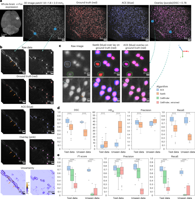
a, Maximum-intensity projection rendering of whole-brain c-Fos expression, with an enlarged view of a cortical patch. Segmentation maps (blue) predicted by the ViT ensemble for the enlarged subregion are shown and compared with GT (red). b, Raw image, GT and segmentation maps for two example image patches, along with voxel-wise uncertainty maps. Regions of high uncertainty are localized around the boundary of sparsely mislabeled processes such as axons (left-hand column) and neuronal somas (right-hand column). Arrows indicate mis-segmented regions from a. c, Qualitative evaluation of segmentation accuracy of ACE versus Ilastik in terms of detection of neurons with low signal intensity or slight blurriness (top), and their shape (bottom). Arrows indicate the boundary of two neurons close to each other. d,e, Quantitative evaluation of the segmentation accuracy of ACE versus Ilastik (d), and detection accuracy of ACE versus Cellfinder (e), in terms of average DSC, precision, recall, HD95 and F1 score on test datasets (n = 12,160 unique patches with 963 ≃ 0.35 mm3) and unseen datasets (n = 1,824 unique patches of 963 ≃ 0.27 × 0.27 × 0.48 mm3). In box plots: box limits, upper and lower quartiles; center line, median; whiskers, 1.5× interquartile range; points, outliers. Mann–Whitney U-test (two-sided), ***P < 0.0001.
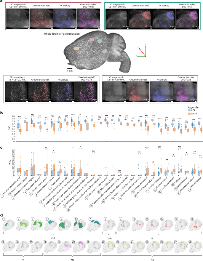
a, Qualitative evaluation of ACE’s segmentation module in different cortical regions in an example subject from the test dataset. Each panel from left to right demonstrates a 3D maximum-intensity projection of a raw (input) image patch, GT (red), model output (blue) and an overlaid version of all three. b–d, On the test set (in total, n = 1,600 unique patches 963 ≃ 0.35 mm3; minimum n = 10 and maximum n = 155 unique patches per region), we registered each LSFM dataset to the ARA using our MIRACL platform’s registration algorithms. ARA labels were then warped to each subject’s native space, with these warped labels then used to determine the location of each image patch in the brain. Average DSC (b) and HD95 (c) were obtained between ACE outputs and GT per ARA label (d) and compared against Ilastik. Box plots: box limits, upper and lower quartiles; center line, median; whiskers, 1.5× interquartile range; points, outliers. Mann–Whitney U-test (two-sided), ***P < 0.001, **P < 0.01, *P < 0.05. CB, cerebellum; CNU, cerebral nuclei; CTX, cerebral cortex; IB, interbrain; MB, midbrain.
To provide a fair comparison against the state-of-the-art segmentation method, Ilastik22, we trained an Ilastik (random forest classifier) model using patches from all training subjects. On our test set, ACE models outperformed Ilastik22 across all experiments. ACE achieved an average improvement in DSC of 0.17 compared with the optimized Ilastik model (P < 0.0001, Mann–Whitney U-test, two-sided; Fig. 2c). ACE showed superior performance in detecting both the boundary and shape of neurons and discriminating neurons that were close to each other, resulting in a lower HD95 (ACE (mean ± s.d.), 4.76 ± 3.47; Ilastik, 9.60 ± 6.78; P < 0.0001, Mann–Whitney U-test, two-sided; Fig. 2c,d). Furthermore, ACE exhibited increased robustness in segmenting neurons with low signal intensity or out-of-focus blurriness (Fig. 2c), while Ilastik struggled to segment these effectively. ACE demonstrated robust segmentation accuracy across different brain regions, and consistently superior segmentation performance (on all evaluation metrics) compared with Ilastik across the whole brain (Fig. 3b and Extended Data Fig. 3). Moreover, ACE achieved higher robustness metrics in simulated distribution shifts (Gaussian noise, smoothing and sharpening) at varying severity levels compared with Ilastik (Extended Data Fig. 4).
To further validate our segmentation model, we compared its performance against the state-of-the-art detection algorithm, Cellfinder33. To this end, we transformed segmentation maps into detection maps by finding the center of mass of each segmented neuron. ACE exhibited superior detection performance, resulting in an F1 score of 0.75 ± 0.08 (mean ± s.d.) versus 0.55 ± 0.15 for Cellfinder (P < 0.0001, Mann–Whitney U-test, two-sided; Fig. 2e). To improve the accuracy of the Cellfinder pipeline on our dataset, we retrained (fine-tuned) the Cellfinder model on our training data and repeated the evaluation experiment. Although retraining elicited an increase of 8.64% in precision compared with the Cellfinder pretrained model, it did not improve overall performance, yielding an overall decrease in F1 score (to 0.28 ± 0.12).
Employing an ensemble of 50 ViTs using the Monte Carlo dropout algorithm improved our baseline model performance, resulting in an average improvement of 2.1% in precision. ACE ensemble models showed high confidence (low uncertainty) in correctly segmented regions, whereas mis-segmented regions demonstrated low confidence (high uncertainty; Fig. 2b). Areas with high uncertainty were typically observed around the boundary of neuronal somas and sparsely mislabeled processes. Voxel-wise uncertainty maps estimate segmentation confidence and can be used in postprocessing to remove potentially FP voxels.
To validate the models’ generalizability, we obtained two unseen (out-of-distribution) datasets with different cell-labeling strategies (transgenic animal for training data versus routine antibody immunostaining for unseen datasets), image resolution, scanning parameters, microscope and image characteristics from those in the training dataset (Extended Data Fig. 2). From unseen dataset 1, we randomly selected 1,820 patches of 963 voxels each (0.27 × 0.27 × 0.48 mm3) and generated silver standard GT data for each image patch. We employed the trained ViT ensemble model and deployed it on the unseen dataset without any fine-tuning or postprocessing (Supplementary Fig. 2). The DSC achieved by our model was 0.73 ± 0.02 (mean ± s.d.) versus 0.45 ± 0.12 for Ilastik (P < 0.0001, Mann–Whitney U-test, two-sided; Fig. 2d). Ilastik segmentations resulted in a substantial number of false negatives (FN) (recall (mean ± s.d.), 0.35 ± 0.15 versus 0.78 ± 0.09 for ACE, P < 0.0001, Mann–Whitney U-test, two-sided; Fig. 2d). Furthermore, ACE outperformed Cellfinder on this unseen dataset (with both the pretrained and fine-tuned model). To ensure a fair comparison, we further conducted Cellfinder runs using various parameters for its detection step, then selected the best model based on a visual comparison (following the authors’ recommendations). This approach allowed us to account for differences in neuronal size distribution and choose the most suitable Cellfinder model for these datasets. Notwithstanding, ACE outperformed the tuned Cellfinder model on all evaluation metrics (P < 0.0001, Mann–Whitney U-test, two-sided; Fig. 2e). Similarly, for unseen dataset 2, the qualitative and quantitative results highlight ACE’s superior performance (P < 0.0001, Mann–Whitney U-test, two-sided; Extended Data Fig. 5) compared with Ilastik and Cellfinder, underscoring the generalizability of our DL models to diverse imaging conditions.
To further increase ACE’s robustness on unseen data, we employed an additional layer of ensembling by combining our optimized ViT and U-Net ensemble models, generating an ‘ensemble of ensembles’ (Supplementary Table 1 shows inference time comparison between ACE and existing algorithms). Our segmentation module thereby takes advantage of a CNN-based architecture that extracts local features within the image patch and a ViT architecture to learn long-range dependencies across the patch. The ensemble of ensembles strategy increased generalizability when dealing with the unseen dataset, improving DSC by an average of 2.1%, precision by 5.2% and decreasing average HD95 by 15.4%. In detection mode, ACE’s ensemble of ensembles increased F1 score by an average of 5.1% and precision by 11.1%. Through fine-tuning of scripts, ACE is generalizable to LSFM data from other cellular markers with different morphological features compared with c-Fos (Extended Data Fig. 6a). To demonstrate the validity of this adaptation, we utilized another dataset of in situ fluorescence imaging of the targets of a covalent drug (pargyline) in intact brain tissue at the subcellular level. We randomly cropped 300 image patches with 963 voxels each (0.17 × 0.17 × 0.19 mm3) from this dataset and generated silver GT data for them. We fine-tuned the ViT model on half of these patches and used the other half for evaluation. The fine-tuned ensemble model achieved a DSC of 0.74 ± 0.14 (mean ± s.d.; Extended Data Fig. 6), indicating robust performance even with different cellular markers and morphologies.
Mapping ensembles orchestrating cold-induced food seeking
Understanding the neural mechanisms governing cold-induced food seeking is crucial for unraveling the intricate interplay between environmental stimuli, energy expenditure and feeding behavior in mammals45,46,47. Our group has recently employed whole-brain c-Fos screening (via SHIELD and LSFM) of mice following prolonged (6-h) exposure to a temperature of either 4 or 30 °C (n = 4 per group), to map the neuronal ensembles that drive cold-induced food seeking48. Our findings highlight selective activation during prolonged cold exposure of the xiphoid nucleus (Xi), a small midline thalamic subregion lacking predefined ARA boundaries, suggesting that Xi plays a key role in mediation of food seeking in response to cold stress48. However, in this previous work, we manually identified the activation of Xi within the ventral midline thalamus based on our initial assumptions and a priori hypotheses. Notably, in this screen, we had relied on ROI-based metrics (including regions encompassing or surrounding Xi) rather than on localized statistics, due to the lack of tools able to generate cluster-wise statistical maps. Here, to validate our pipeline’s ability to automatically detect selective activation of specific neuronal populations at the subregional level in an unbiased manner, we analyzed this whole-brain c-Fos LSFM dataset using ACE.
We first utilized ACE’s models to generate whole-brain segmentation maps (Fig. 4a). To maintain data fidelity and prevent information loss during warping into a common reference with lower resolution, we applied a convolution-based voxelization procedure to the maps based on our previous work10. Following voxelization, segmentation maps were aligned with ARA at 10-µm resolution using deformation fields obtained via our MIRACL platform’s registration module (Fig. 4b,c and Supplementary Fig. 3). To identify neural activity hotspots, we generated group-wise heatmaps of neuronal density by subtracting the average of the voxelized and warped segmentation maps in each group (Fig. 4d). These heatmaps revealed that cold stress elicited increased neuronal activity within the hypothalamus, consistent with its role in thermoregulation49, and attenuated neuronal activity across the cortex, probably due to reduced physical activity during cold exposure48,50.
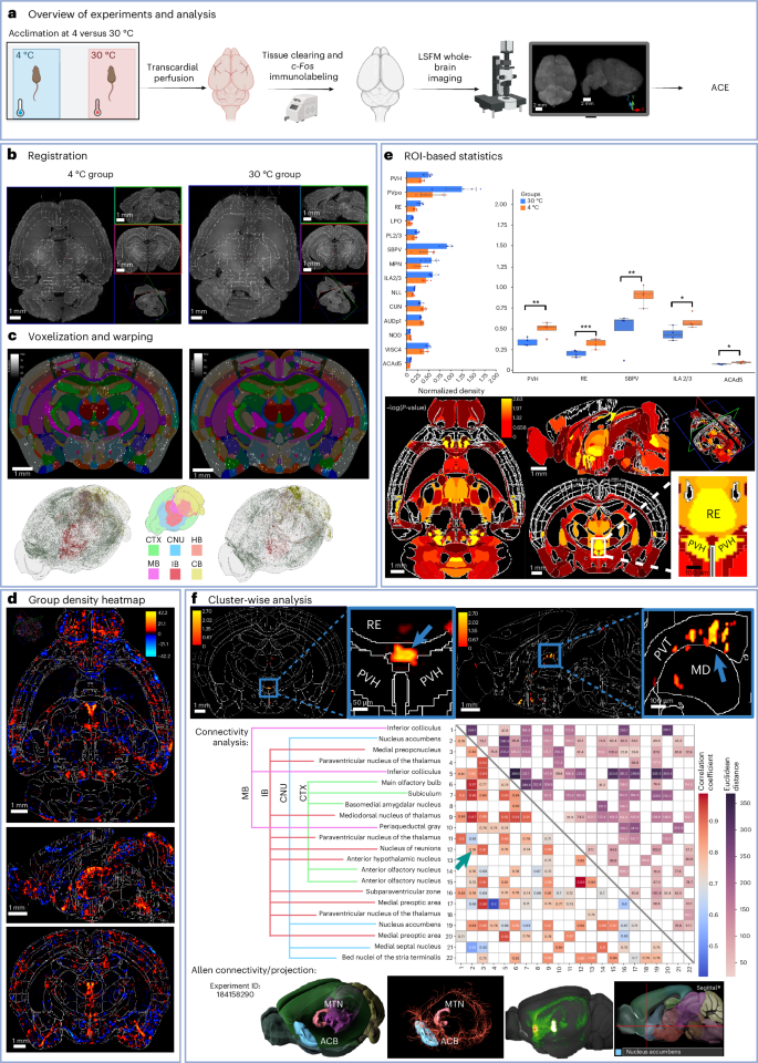
a, Experimental design (n = 4 per group). b, LSFM data were registered to the ARA using MIRACL. Left and right panels show autofluorescence data overlaid on labels for two subjects in each group. c, Segmentation maps from ACE were voxelized to ARA 10-µm resolution; voxelized maps were then warped to ARA. Top, one subject per group overlaid on labels; bottom, 3D rendering of segmentation maps color coded based on six regions: cerebral cortex (CTX), cerebral nuclei (CNU), midbrain (MB), hindbrain (HB), interbrain (IB) and cerebellum (CB). d, Segmentation maps were averaged and then subtracted to obtain group-wise heatmaps. e, An independent t-test (two-sided) was applied between c-Fos+ density per label for ROI-wise analysis (n = 4 per group). Top left, trending ROIs (P < 0.1); top right, significant regions (***P > 0.001, **P < 0.01, *P < 0.05); bottom, corresponding P values per label. Box plots: box limits, upper and lower quartiles; center line, median; whiskers, 1.5× interquartile range. Data are presented as mean ± s.d. f, ACE cluster-wise analysis (two-way ANOVA). Top, significant clusters within the midline group of the dorsal thalamus (MTN), including one cluster close to the Xi region between the paraventricular nucleus of the hypothalamus (PVH) and above the third ventricle (left); and multiple clusters in the dorsal subregion of the paraventricular nucleus of the thalamus (PVT, right). Middle, Pearson correlation (significant correlations only, P < 0.01, bottom left triangle) and Euclidean distance (top right triangle) between the 22 significant clusters, ranked according to activation strength. Arrow indicates correlation between one cluster located in the nucleus of reuniens (RE) and another in the nucleus accumbens (ACB). Bottom, 3D connectivity maps derived from anterograde viral vector (AAV) tracing from an experiment (ID 184158290) in the ARA, demonstrating structural connectivity between the RE in MTN and ACB. Panels, from left to right, show (1) MTN and ACB, (2) fibers originating from RE and projecting into ACB, (3) maximum-intensity projection and (4) a sagittal view of the atlas. a was created using BioRender.com.
For assessment of between-group differences, we first conducted ROI-wise analysis between the two groups within each atlas region (Fig. 4e). This whole-brain analysis highlighted several brain regions that exhibited significant differential activation (P < 0.05, Student’s paired t-test, two-sided), notably the paraventricular hypothalamic nucleus and the nucleus of reuniens (Fig. 4d). Some areas showed diverging group trends but did not reach significance, including the cuneiform, a region involved in locomotion51, and primary auditory cortex. Multiple comparison corrections were not performed, following common practices of whole-brain, ROI-based analysis, due to the very large number (>1,100) of ARA regions, highlighting another key limitation of such analysis. A visual inspection of the group-difference heatmap revealed that the ROI-based analysis on predefined atlas regions failed to detect several highly localized areas with substantial increases in c-Fos activation in the cold group—most notably within the large nucleus of reuniens (Fig. 4d).
For testing of whether ACE could map localized group-wise differences in neuronal activity in an atlas-agnostic manner, we employed ACE’s cluster-wise TFCE permutation test using group-wise ANOVA. ACE extracted clusters of activation across the whole brain (Fig. 4f) and summarized and ranked each cluster by its strength of activation, total volume and percentage volume within each overlapping brain region (Supplementary Table 2). Our statistical and visualization tools not only highlighted expected areas of c-Fos activation, but also identified numerous previously undetected subregional changes in the cold-induced dataset: for instance, clusters located only within the dorsal subregion of the paraventricular nucleus of the thalamus (PVT, Fig. 5), which were missed in the ROI-based analysis using the (whole) PVT region (ARA label; Fig. 4f and Supplementary Table 2). Utilizing ACE’s native space cluster validation algorithm (Fig. 5 and Supplementary Table 2), we warped the clusters found in the paraventricular nucleus into the native space of each subject. We found that the number of c-Fos+ cells was significantly higher (P< 0.05, Mann–Whitney U-test, two-sided; Supplementary Table 2) in the cold-induced group compared with the control group (for example, for one cluster the neuronal count in the cold-induced group was 23 ± 8 (mean ± s.d.) versus 6 ± 2 for the control). In contrast to the ROI-based analysis, our cluster-wise test revealed a significant (P < 0.01, group-wise two-way ANOVA; Supplementary Table 2) localized increase in c-Fos activation in the ventral midline of the nucleus of reuniens and above the third ventricle, corresponding to the Xi, and confirming its recently established role in the neural orchestration of cold-induced food-seeking behavior and energy homeostasis. We also performed connectivity analysis between significant clusters, assessing the correlation of their activations (using Pearson correlation analysis with permutation and bootstrapping; Fig. 4f). We observed significant associations (P < 0.01, correlation test with permutation) between clusters in the midline group of the dorsal thalamus (including paraventricular nucleus and Xi) and the nucleus accumbens—that is, putative regional connectivity, which was validated by anterograde viral tracing48 using the Allen connectivity atlas (Fig. 4f).
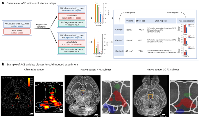
a, Overview of the validation algorithm. Significant clusters identified through ACE’s cluster-wise TFCE permutation-based statistical algorithm were binarized and underwent a connected component analysis to differentiate each cluster. The processed significant clusters were then warped to the native space of each subject using registration deformation fields. Using ACE segmentation maps, the number of neurons within each cluster was computed. A Mann–Whitney U-test (two-sided) was used to compare the number of neurons within each cluster between the two groups. The number of neurons per subject for each cluster—in addition to their volume, effect size, atlas space P value (obtained via ACE cluster-wise TFCE permutation), brain regions they spanned and native space P value (obtained via post hoc Mann–Whitney U-test)—are summarized. b, Validation of neuronal ensembles detected by ACE cluster-wise analysis in the food-seeking behavior experiment. From left to right, axial view of the cluster-wise P value map, overlaid on ARA label boundaries at a resolution of 10 µm; zoomed view of significant clusters in PVT. The P value map was warped back into the native space of randomly selected subjects of the 4 and 30 ° groups using the deformation matrices obtained by registration; corresponding axial views from subjects in the 4 and 30 °C groups, respectively, and zoomed versions of cluster boundaries in PVT, showing higher c-Fos+ activity in the 4 versus 30 °C condition in the clusters detected in atlas space. Cluster colors in native space (columns 2 and 3) correspond to the manually drawn boundary in atlas space (column 1), for visual comparison. NS, not significant.
Mapping of brain-wide local neuronal activation
Locomotive behavior is a complex process that involves coordinated neuronal activity in different areas of the brain52. Identification of laminar neuronal ensembles that underlie locomotion represents an ongoing challenge in neuroscience1. We deployed ACE to map local neuronal activation during walking versus homecage using c-Fos (n = 3 per group). Segmentation maps obtained from ACE (Extended Data Fig. 7a,b) were voxelized and warped to 10-µm ARA (Extended Data Fig. 7c). Group-wise heatmap intensity analysis (Extended Data Fig. 7d) and whole-brain ROI-based comparison showed an increase in c-Fos+ density in the primary motor areas (MOp) and secondary motor areas in the walking versus homecage group (P < 0.05, Student’s paired t-test, two-sided; Extended Data Fig. 7d). We repeated ROI-based analysis at depth 6 by merging ARA regions using the atlas’s hierarchical structure (Extended Data Fig. 8a,b), a strategy used to enhance sensitivity or address lower-resolution data53. We identified major areas with elevated c-Fos+ density, including somatomotor areas (secondary motor areas; P < 0.05, Student’s paired t-test, two-sided). To test whether ACE could detect subregional changes, we used our cluster-wise TFCE algorithm, demonstrating layer-specific areas of c-Fos activation in both MOp and secondary motor areas (Extended Data Figs. 7e, 8c and 9 and Supplementary Table 3). We identified clusters confined to a single layer in somatomotor areas, including (1) MOp layer 6a, where thalamocortical projections from the motor thalamus were observed using anterograde viral tracing54 and (2) clusters spanning multiple layers within the MOp and retrosplenial areas (Extended Data Figs. 8c and 9b). Notably, our algorithm (Extended Data Fig. 10) detected localized clusters in the lateral hypothalamic area (LHA) and midbrain reticular nucleus that the whole-brain and depth 6 ROI-based analyses failed to detect (Extended Data Fig. 8a,b). Using our validate clusters algorithm, we found higher LHA c-Fos+ cell densities in the walking group versus homecage in the detected regions identified by ACE (Extended Data Fig. 7f and Supplementary Fig. 4), highlighting its potential role in movement.
Discussion
This work introduces ACE, an automated end-to-end pipeline for mapping of neuronal ensembles at the subregional level in teravoxel-scale LSFM data.
Our large training dataset and cutting-edge architectures enabled ACE models to learn variations in image characteristics of labeled cells and imaging artifacts across different regions and subjects, surpassing traditional techniques1,21,55,56 that require parameter tuning. Due to the modular nature of the pipeline, ACE is extendable to different imaging modalities, including multiphoton microscopy data and 3D histology stacks, via fine-tuning modules available within the pipeline. Notably, ACE could be used to study connectivity via quantification of neuronal soma in upstream regions using retrograde adeno-associated virus viruses.
Our cluster-wise methodology, optimized for whole-brain LSFM data, comprehensively characterizes activity ‘hotspots’ while enhancing sensitivity and statistical power. Although increased FP in voxel-wise tests may be addressed through multiple correction methods1,10,56 or manual cluster definition and subsequent post hoc analyses for validation56, these approaches limit algorithm sensitivity. Our cluster-wise permutation analysis distinguishes itself for its automatic, data-driven cluster definition by leveraging neighborhood information, mitigating the need for data-specific expertise and minimizing bias in statistical analysis. Other key advantages to our statistical pipeline are an advanced native space cluster validation algorithm and the ability to account for covariates or perform mixed-effects modeling at the cluster level, which has not been implemented in existing tools.
When studying food seeking following cold stress, our results align with ROI-based semiautomated studies of c-Fos activation46,48. However, we uncovered localized changes in neural activity that may have gone unnoticed in ROI-based analyses46,48. ROI-based analyses may overlook subtle changes because effects, and hence significance, are estimated by averaging over the entire region. Voxel-wise methodologies are overly reliant on the intensity of individual voxels. In contrast, our approach provides a more granular understanding of neural activity patterns, offering enhanced specificity to detect nuanced changes in brain activity over small areas.
Gaining circuit-level insights based on specific neuronal populations is key to unraveling the organizational principles of the motor system52,57. Our findings on locomotion-elicited neuronal activity align with other studies52, wherein c-Fos density increased in areas such as MOp and cuneiform nucleus (CUN). Our previous work, using manual parameter tuning and postprocessing of c-Fos+ data, virus tracing and photostimulation, identified a subpopulation of neurons in the LHA that may play a role in walking recovery following chronic lateral hemisection spinal cord injuries. Here, we have shown increased activity restricted to a subregion localized within the LHA that probably contributed to the failure of ROI-based analysis to detect LHA activation, or remained un-noticed in studies utilizing a more limited approach of narrowing down c-Fos analysis to a few key ROIs associated with locomotion or combining ROIs into larger areas. This distinctive capability enables our pipeline to surpass the limitations of ROI-based methods, and facilitates a comprehensive and unbiased exploration of the intricate organization of brain networks.
Artficial intelligence-based cartography of ensembles provides a quantitative approach to mapping of locally activated regions in an atlas-agnostic fashion, which is particularly beneficial in experiments exploring brain areas that lack standard or high-resolution digital atlas parcellations. The resulting maps can serve as a basis for creating and refining high-fidelity functional atlases. Leveraging the statistical module and correlation analysis, ACE facilitates the extraction of associations among clusters of activations, potentially revealing long-range connectivity or functional coherence.
While this study primarily focused on the development and validation of a pipeline for mapping neuronal activity in LSFM data using immediate early genes, our fine-tuning functions allow ACE to adapt to other fluorescent reporters. However, in multilabeled datasets in which different fluorescent labels represent distinct genotypes (as seen in mosaic markers54,58), our fine-tuning algorithms may not produce optimal results. Although our models were trained on teravoxel LSFM, segmentation errors may still occur, biasing statistical results, particularly around sparsely mislabeled processes. This phenomenon might be, in part, attributed to the use of silver GT data; however, manual annotaton of tens of thousands of patches is impractical and unscalable. We developed the ensemble of ensembles model to deal with potential FP on unseen datasets, increasing segmentation performance. While our statistical approach using TFCE does not require predefined, cluster-forming thresholds, it utilizes free parameters. Consistent with other studies44,59, fixing these TFCE parameters yields robust outcomes for LSFM analyses, because the same parameters were applicable to both food-seeking and walking experiments. Nevertheless, the use of suboptimal parameters may lead to an increased number of FP or FN44,60.
In summary, ACE offers a streamlined approach for achieving high-fidelity, unbiased, 3D mapping of local and laminar neuronal ensembles across the entire brain, independent of predefined atlas regions. ACE’s DL models are notable for their ability to provide generalizable segmentation of neuronal somas in teravoxel LSFM data. Integration with the MIRACL registration workflow, coupled with ACE’s statistical module, establishes a framework for identifying and discovering differentially activated localized clusters of ensembles in response to experimental manipulations, which has not proved feasible to date. This comprehensive tool has the potential to empower researchers to study neural activity patterns at an unprecedented level, providing valuable insights that might be obscured using traditional ROI-based or voxel-wise analysis. ACE is applicable across a wide range of LSFM datasets and neuroscience paradigms, and is made freely available through our MIRACL platform, thus boosting our understanding of neural ensembles orchestrating behavior and cognition.
Methods
Datasets and experiments
Training dataset
Our training data consisted of two LSFM cohorts of TRAP2-Ai9 mice (total n = 18): (1) ten animals aged 3–4 months with whole-brain data acquired and (2) eight animals aged 2 months with data acquired from the left hemisphere. All animal procedures followed animal care guidelines approved by the Institutional Animal Care and Use Committee at the Scripps Research Institute. These animals had an immediate early gene (c-fos) promoter, contributing to the activity-dependent expression of inducible recombinase Cre-ERT2. The expression of fluorescent protein tdTomato was activated following the injection of 20 mg kg−1 4-hydroxytamoxifen. We used the following splits for training and evaluation: the training set consisted of ten animals, with three and five used for the validation and test sets, respectively.
Unseen dataset 1
We used whole-brain LSFM data from a model of spinal cord injury (n = 3 mice) to validate our DL segmentation models. Briefly, mice were induced under anesthesia with a mixture of isoflurane and O2. Mice were then placed on a heating pad set to 37 °C and maintained on 1–3% isoflurane and O2. A midline skin incision was made and the T10 lamina identified. A T10 laminectomy was performed, followed by left lateral hemisection using either microscissors or a microscalpel61. Muscle closure was performed with 6-0 Vicryl followed by skin closure with 6-0 Ethilon. Postoperatively, mice were placed on a heating pad and given subcutaneous fluids as needed. Pain control for 48 h postoperatively was also provided via subcutaneous daily administration of Rimadyl (5 mg/kg−1). Bladders were expressed twice daily until spontaneous recovery of bladder function. All hemisection lesions were histologically confirmed as adequate. All three mice were adult female C57BL/6 mice (≥8 weeks of age at the start of the experiment, 15–30 g body weight). All procedures were performed in compliance with the Swiss Veterinary Law guidelines and were approved by the Veterinary Office of the Canton of Geneva, Switzerland (license no. GE/112/20).
Unseen dataset 2
We used whole-brain LSFM data obtained from a male C57BL/6 J mouse (Jackson Laboratory, strain 000664), aged 18 months. All animal procedures followed protocols approved by the Stanford University Institutional Animal Care and Use Committee, and met the guidelines of the National Institutes of Health Guide for the Care and Use of Laboratory Animals.
Cold dataset
We analyzed the cold and thermoneutral c-Fos dataset from our previous publication48. Briefly, single-housed male wild-type (WT) C57BL/J6 mice were exposed to either 4 °C (cold) or 30 °C (thermoneutral) for 6 h, with free access to food and water, before perfusion. Mouse brains were harvested and fixed in 4% paraformaldehyde (PFA) following perfusion.
Walking dataset
We used two groups of adult female C57BL/6 mice (≥8 weeks of age at the start of the experiment, 15–30 g body weight, n = 3 per group). Briefly, mice were trained to run quadrupedally on a treadmill (Robomedica, Inc.) 5 days per week for 2 weeks before perfusion. To elicit c-Fos expression, mice ran on the treadmill for 45 min at a speed of 9 cm s−1 and were then perfused for 1 h (walking group). Mice in their home cages were perfused for homecage group analysis.
Fine-tuning dataset
We used LSFM data from a hemisphere of a mouse brain. The clearing-assisted tissue click chemistry method was used for in situ fluorescence imaging of drug molecules that bind to specific targets. In this method, the covalent monoamine oxidase inhibitor pargyline-yne was administered to the mouse at a dose of 10 mg kg−1 for 1 h by intraperitoneal injection. The drug was labeled with AF647 dye using a click reaction, allowing us to visualize drug molecules within brain tissue.
Tissue clearing and immunolabeling
Training dataset
Two weeks following injection of 4-hydroxytamoxifen, mice were perfused; their brains were collected and underwent overnight fixation in 4% PFA solution. Fixed brain specimens were treated using the SHIELD8 protocol to maintain the integrity of protein antigenicity. Thereafter, an active clearing procedure was used for tissue CLARITY5. Samples were index matched by adding them to EasyIndex medium before imaging with a light-sheet microscope.
Unseen dataset 1 and walking dataset
Adult mice were anesthetized with intraperitoneal pentobarbital (150 mg kg−1), followed by intracardiac perfusion of 1× PBS then 4% PFA in PBS. The brain was dissected and the sample postfixed in 4% PFA overnight at 4 °C. Brains then underwent processing with iDISCO+ (ref. 1). Briefly, samples underwent methanol pretreatment by dehydration with a methanol/H2O series, each for 1 h, as follows: 20, 40, 60, 80 and 100%. Samples were then washed with 100% methanol for 1 h and chilled at 4 °C, followed by overnight incubation in 66% dichloromethane/33% methanol at room temperature. This was followed by two washes in 100% methanol at room temperature, then bleaching in chilled fresh 5% H2O2 in methanol overnight at 4 °C. Samples were rehydrated with a methanol/H2O series as follows: 80, 60, 40 and 20% then PBS, each for 1 h at room temperature. Samples underwent washing for 2× 1 h at room temperature in PTx.2 buffer, and were then incubated in permeabilization solution for 2 days at 37 °C. Samples were then incubated in blocking solution (42 ml of PTx.2, 3 ml of normal donkey serum and 5 ml of DMSO, for a total stock volume of 50 ml) for 2 days at 37 °C with shaking. This was followed by incubation in a primary antibody solution consisting of PBS/0.2% Tween-20 with 10 μg/ml heparin (PTwH), 5% DMSO, 3% normal donkey serum and c-Fos (rabbit anti-c-Fos, 1:2,000, Synaptic Systems, catalog no. 226003) for 7 days at 37 °C with shaking. Next, samples were washed in PTwH for 24 h, followed by incubation in a secondary antibody solution consisting of PTwH, 3% normal donkey serum and donkey anti-rabbit Alexa Fluor 647 (1:500, Thermo Fisher Scientific) for 7 days at 37 °C with shaking. Samples were then washed in PTwH for 24 h, followed by tissue clearing; final clearing was performed using iDISCO+ (ref. 1). Briefly, samples were dehydrated in a methanol/H2O series as follows: 20, 40, 60, 80 and 100%, each 2× 1 h at room temperature. This was followed by a 3-h incubation in 66% dichloromethane/33% methanol at room temperature, then incubation in 100% dichloromethane for 2× 15 min. Samples were then incubated in dibenzyl ether for at least 24 h before imaging.
Cold dataset
Whole-brain clearing was performed by LifeCanvas Technologies through a contracted service. To preserve samples’ protein architecture, they were fixed with proprietary SHIELD8 solutions from LifeCanvas Technologies. Samples were then placed in the SmartBatch+ system to carry out active clearing and immunolabeling with rabbit anti-c-Fos primary antibody (CST, catalog no. 2250S). Samples were index matched by placing them in EasyIndex medium.
Unseen dataset 2
The animal was anesthetized with isoflurane and transcardially perfused with PBS, followed by 4% PFA. The whole mouse brain was extracted carefully and fixed in 4% PFA for 24 h; the PFA-fixed sample was then processed using the SHIELD8 protocol (LifeCanvas Technologies). Active clearing of samples was carried out using the Smartbatch+ device. Samples were then immunolabeled using eFLASH62 technology, incorporating the electrotransport and SWITCH63 methods. Samples were labeled with a recombinant anti-c-Fos antibody (abcam, catalog no. ab214672) and then fluorescently conjugated with Alexa Fluor 647 (Invitrogen, catalog no. A-31573) at a primary:secondary molar ratio of 1.0:1.5. Following labeling, samples were index matched (n = 1.52) by incubation in EasyIndex medium (LifeCanvas Technologies).
LSFM imaging
Training dataset
Samples were index matched with EasyIndex medium and imaged on a light-sheet microscope (SmartSPIM) with a ×4 objective lens. For eight subjects, data were acquired from a hemisphere while, for the remainder, data were acquired from the whole brain. Nominal lateral spatial resolution was 3.5 µm, and step size was set to 4 µm in the z-direction, with 561-nm excitation and an emission filter of 600/52 nm.
Unseen dataset 1 and walking dataset
Imaging of whole brains was performed using a CLARITY-optimized light-sheet microscope, as previously described64, with a pixel resolution of 1.4 × 1.4 µm2 in the x and y dimensions and a z-step of 5 µm, respectively, using the ×4/0.28 (numerical aperture) objective, which is suitable for resolving cell nuclei labeled by c-Fos. Using a custom-made quartz cuvette filled with dibenzyl ether, whole brains were imaged. Two channels were imaged: one with autofluorescence (auto channel, 488 nm) to demonstrate anatomy, and a second demonstrating c-Fos labeling (cell channel, 647 nm). All raw images were acquired as 16-bit TIFF files and were stitched together using TeraStitcher65.
Cold dataset
Whole-brain imaging and automated analysis were performed by LifeCanvas Technologies through a contracted service. Samples were index matched by placing them in EasyIndex medium, and imaged on a light-sheet microscope (SmartSPIM) with a ×4 objective lens. Nominal lateral spatial resolution was 1.75 µm, and step size was set to 4 µm in the z-direction.
Unseen dataset 2
The index-matched (n = 1.52) whole-brain sample was imaged using a SmartSPIM light-sheet microscope. The sample was imaged with a ×4 objective lens. Samples were imaged with a 642-nm laser. Nominal lateral spatial resolution was 1.8 µm, and step size was set to 4 µm in the z-direction
GT label generation
Our annotation strategy for generating silver standard GT labels of neuronal somas comprised three stages: MIRACL10 segmentation, Ilastik pixel classification and postprocessing.
MIRACL segmentation
To create GT labels, we first used the MIRACL10 segmentation workflow that incorporates image-processing tools implemented as FIJI/ImageJ macros38. The workflow includes a 3D watershed marker-controlled algorithm and a postprocessing 3D shape filter to omit FP. This resulted in binary GT labels across the entire dataset with a low FP rate and relatively higher FN rate.
Ilastik pixel classification
To improve MIRACL-generated GT labels we used Ilastik22, which performs pixel classification using image filters (as input features) and a random forest (RF) algorithm (as a classifier) through a user-friendly interface. Filters include pixel color and intensity descriptors, edginess and texture in 3D and at different scales. The RF combines hundreds of decision trees and trains each one on a slightly different set of features. The final predictions of RF are made by averaging the predictions of each tree. We used 37 three-dimensional filters and an RF classifier with 100 trees. To train the RF classifier, we imported MIRACL’s segmentation outputs as silver input annotations (initialization) to Ilastik (that is, in lieu of manual annotations). To address the prohibitive speed and memory requirements of the RF algorithm, we trained it on image patches (5123 voxels). For each brain, three 5123 patches from different depths were randomly selected. The RF model was trained several times by providing feedback (that is, by correcting the results with expert annotation and modifying the labels to achieve optimal results). Ilastik output did not correctly detect the boundaries of neuronal soma, and frequently overestimated their spatial extent.
Postprocessing
To further reduce the number of FP voxels in GT labels, we applied a 3D shape filter using the ImageJ shape filter plugin66 on Ilastik-generated labels. To solve the problem of volume overestimation, we applied a 3D erosion filter with a sphere-like kernel (radius of one voxel) to the GT labels. The final whole-brain GT labels were visually quality checked in three 5123 patches per brain, by two raters; specifically, the raters were asked to randomly select and validate one 5123 patch in the cerebrum, brain stem and cerebellum.
Deep neural network architectures
ACE’s segmentation module consisted of 3D ViT-based and CNN-based (U-Net) architectures (Extended Data Fig. 1).
UNETR
The popular U-Net architecture has powerful representation learning capabilities, and generates more accurate dense-segmentation masks than do other CNN architectures (such as Mask R-CNN), thanks to the preservation of spatial information26,67. However, fully convolutional models are limited in their ability to learn long-range dependencies, resulting in potentially suboptimal segmentation of objects in large volumes, including neuronal cell bodies of varying shape and size (for example, in different regions of the brain). To address this issue, a ViT architecture (UNETR) has been proposed in which the encoder path of a U-Net is replaced by a transformer to learn contextual information from the embedded input patches68. This motivated us to develop and deploy optimized UNETR-based segmentation models with residual blocks and dropout layers to improve the robustness and generalizability of previous pipelines. Specifically, in UNETR68 the encoder was replaced with a stack of 12 transformer blocks, operating on a 1D sequence (163 = 4,096) embedding of the input (one channel 3D image patch, 963 ≃ 0.27 × 0.27 × 0.48 mm3). Subsequently, a linear layer projected the vectors into a lower dimensional embedding space (embedding size K = 768), which remained constant throughout the transformer layers. A 1D learnable positional embedding was added to the projected patch sequence to preserve spatial information. This embedded patch sequence, with the dimension of N × K (N is the sequence length and N = H/16 × W/16 × D/16 × K and H, W and D are the 3D input’s height, width and depth), was passed as input to the stack of transformer blocks. Each transformer block consisted of multihead attention and multilayer perceptron layers. All multihead attention modules consisted of multiple self-attention heads, where each self-attention block learned mapping in the patch sequence in parallel. We extracted learned sequence representations at four different depths of the transformer stack and reshaped each back to (scriptstylefrac{H}{16}times frac{W}{16}times frac{D}{16}times K). The embedded sequence vectors then underwent five different encoder blocks with consecutive convolutional layers to achieve supervision at different depths (Extended Data Fig. 1).
The encoder was connected to a decoder via skip connections at multiple resolutions, to predict segmentation outputs. We developed an optimized UNETR68 architecture with some modifications, including the addition of dropout layers in all blocks and residual units69 in convolution blocks in the encoder, as a regularization strategy to avoid overfitting and vanishing gradient problems. For a given 3D input cube, the segmentation models generated a 3D volume containing voxel-wise probabilities of neuronal cell bodies (0 < P < 1). Prediction maps were binarized using either a default (0.5) or user-fed threshold to generate a map representing whether a voxel belongs to a neuron.
U-Net
We similarly implemented an optimized version of the seminal U-Net70,71,72 architecture, with some modifications, based on our previous work40. The U-Net architecture consists of contracting (encoder) and expanding (decoder) paths. The encoder is based on 3D convolution and pooling operators; it takes an image patch as input and generates feature maps at various scales, creating a multilevel, multiresolution feature representation. Meanwhile, the decoder with up-convolution operators leverages these feature representations to classify all pixels at the original image resolution. The decoder assembles the segmentation, starting with low-resolution feature maps that capture large-scale structures, and gradually refines the output to include fine-scale details. In our U-Net architecture, the standard building blocks have been replaced with a residual block69. In addition, parametric rectifying linear units73 have been deployed to provide different parameterized nonlinearity for different layers. We converted all 2D operations, including convolution and max-pooling layers, into 3D and used batch normalization rather than instance normalization to achieve a stable distribution of activation values throughout the training, and to accelerate training74. A dropout layer was added between all convolution blocks in the architecture as a regularizer, to avoid overfitting36,75. Except for the first residual units, all convolutions and transpose convolutions had a stride of 2 for downsampling and upsampling, respectively. The first residual unit used a stride of 1, which has been shown to increase performance by not immediately downsampling the input image patch70.
All brain light-sheet data are first divided into smaller image patches. Deploying ACE segmentation models, binary and uncertainty maps are obtained per image patch; the pipeline then automatically stitches all the maps to create whole-brain segmentation and uncertainty maps that match the input data.
Loss function
The DSC is a widely used metric that measures similarity between two labels. The class average of the DSC can be computed as
where N is the number of classes, K is the number of voxels and GTk,n and Pk,n denote GT and output prediction, respectively, for class n at voxel k.
Cross-entropy (CE) measures the difference between two probability distributions over the same sets of underlying events, and was computed as
In regard to ACE DL architecture, we used an equally weighted Dice–cross-entropy loss, which is a combination of Dice loss and cross-entropy loss functions; this was computed in a voxel-wise manner as
Model training
To train our DL models, we used a total of 36,480 unique input patches (963 voxels), not accounting for data augmentation. To address the issue of class imbalance in our dataset (the majority of voxels representing background), patches containing only background—or a small number of foreground voxels (<100,000)—were filtered out from the 5123 image patches generated by the annotation strategy. Hence, for the UNETR model with an input size of 963, we used 15,200, 9,120 and 12,160 unique input patches (not accounting for data augmentation) for training, validation and testing, respectively (n = 30,400 patches with augmentation for training alone); for the U-Net model with an input size of 1283, we used 7,600, 3,840 and 5,120 patches, respectively.
For hyperparameter tuning, we used a Bayesian optimization approach via the Adaptive Experimentation Platform (https://ax.dev/). The following hyperparameters were optimized during training: input image size, encoder and decoder depth, kernel size, learning rate, batch size, kernel size and loss function. For the UNETR architecture, which in total had 92.8 million parameters, the best model based on DSC performance on the validation set had the following parameters: 12 attention heads, feature size of 16, input patch size of 963 voxels and batch size of 24. The U-Net architecture, which in total had 4.8 million parameters, had the following parameters: a five-layer encoder with an initial channel size of 16 and kernel size of 3 × 3 × 3, input patch size of 1283 voxels and batch size of 27.
The UNETR and U-Net models were trained for 700 and 580 epochs, respectively. To avoid overfitting, early stopping was set to 50 epochs where performance (DSC) on the validation dataset did not improve. The Adam optimizer76 was used with an initial learning rate of 0.0001.
Implementation
All DL models were implemented in Python using the Medical Open Network for Artificial Intelligence framework (MONAI77), and the PyTorch machine learning framework78. All training was performed on the Cedar and Narval cluster provided by the Digital Research Alliance of Canada (www.alliancecan.ca), using NVIDIA V100 Volta graphic processing units with 32 GB of memory, and A100 graphic processing units with 40 GB of memory. Registration of our data to ARA was performed with our in-house, open-source MIRACL10 software. MIRACL is fully containerized and available as Docker and Singularity/Apptainer images (https://miracl.readthedocs.io/). For results visualization, we used a variety of open-source software applications and Python libraries, including matplotlib, seaborn, Brainrender79, Fiji/ImageJ38, itk-SNAP80 and Freeview (http://surfer.nmr.mgh.harvard.edu/). We also used BioRender for figure creation in this manuscript (https://www.biorender.com/).
Data augmentation
To increase the generalizability of the DL model and model distribution shifts in LSFM data, the training set images were randomly augmented in real time at every epoch. Supplementary Fig. 3 shows all the data augmentation transforms used, namely: affine transformations, contrast adjustment, histogram shift, random axis flipping and different noise distributions such as salt and pepper, and Gaussian. These transforms were selected because they are representative of distortions that occur during LSFM imaging. Briefly, a range (0, 1) of scaling was applied to each 5123-image patch, based on the intensity distribution of that patch. The intensity of each 5123-image patch was scaled from the [0.05, 99.5] percentile to [0, 1], where 0.05 and 99.95 are the intensity values at the corresponding percentiles of the image patch. Subsequently, each data augmentation transform was randomly applied (with a probability of P = 0.5) to the 5123-image patch at each epoch. The parameters of each data augmentation were also randomly selected at each epoch from the predetermined range of values.
Voxel-wise uncertainty map
Epistemic uncertainty, as described previously35, is rooted in a lack of knowledge about model parameters and structure, rather than stemming from inherent variability in the observed data; this type of uncertainty is often referred to as model uncertainty35. To estimate the models’ uncertainty and confidence in predictions, we used the Monte Carlo dropout approach. During training, dropout layers (with a probability of P = 0.2) were utilized as a regularization technique. It has been shown that turning on dropout layers (randomly switching neurons off) in inference mode can be interpreted as a Bayesian approximation of the Gaussian process36. At test time, when the dropout layers are turned on, each forward pass yields a stochastically different prediction as a sample from the approximate parametric posterior distribution ((P(,{y}|{X},)))37. This technique has been shown to provide useful insights into the model’s uncertainty, by computing the variance of numerous predictions ((Y={,{y}_{1},{y}_{2},ldots ,{y}_{N},})). Voxel-wise uncertainty (variance) can thus be defined7:
The resulting voxel-wise uncertainty map provides a measure of variation in predictions of slightly different models for the same data, which can be particularly useful in identifying regions of high uncertainty.
Ensemble of ensembles
Each model’s output was obtained by averaging the probability maps of 50 models ((Y=left{,{y}_{1},{y}_{2},ldots ,{y}_{50}right})) using the Monte Carlo dropout technique:
Subsequently, to combine the prediction maps of both models, a final mapping of neurons was generated using an ensemble of both models (ensemble of ensembles):
Model evaluation
Evaluation metrics
To evaluate the performance of the segmentation models, several volume- and shape-based metrics were used, including DSC, recall, precision, F1 score and HD95. We used the metrics derived from the resulting confusion matrix and associated true-positive (TP), FP and FN values. Each neuronal soma was defined as a 3D connected component. Given this definition, TP was defined as the number of correctly detected neurons following comparison of GT with prediction P. Sensitivity or recall measures the proportion of TP relative to the number of individual neurons delineated in GT, and was defined as
Precision measures the proportion of TP against all positive predictions, and was defined as
While recall is useful to gauge the number of FN pixels in an image, precision is useful to evaluate the number of FP pixels in a prediction.
The F1 score combines precision and recall, and is often used to measure the overall performance of a model. The F1 score measures the number of wrongly detected neurons in P:
DSC measures the number of elements common to GT and P datasets, divided by the sum of the elements in each dataset, and is defined as
Hausdorff distance is a mathematical measurement of the ‘closeness’ of two sets of points that are subsets of a metric space; it is the greatest of all distances from a point in one set to the closest point in the other. We used the 95th percentile of Hausdorff distance rather than the maximum results, to provide a more robust and representative measure of the segmentation’s performance in image analysis tasks. Given two sets of points, X and Y, Hausdorff distance between these two sets was defined as
Simulation distribution shift
We deployed our recently published ROOD-MR platform (https://github.com/AICONSlab/roodmri) on our test data, which includes methods for simulating distribution shifts in datasets at varying severity levels using imaging transforms and generating benchmarking segmentation algorithms based on robustness to distribution shifts and corruptions. We employed three commonly used transforms that disrupt low-level spatial information (Gaussian noise, smoothing and sharpening). We added Gaussian noise to the image with zero mean and 0 < σ < 1. For sharpening, we used a Gaussian blur filter with a zero mean and 0.05 < σ < 2. We also applied a Gaussian smooth filter to the input data based on the specified sigma (σ) parameter (0.05 < σ < 2).
Comparison against Ilastik
We used the pixel classification module in Ilastik and trained a RF classifier using all training subjects (18 whole-brain LSFM images). We used 37 three-dimensional filters and an RF classifier with 100 trees. To train the RF model, we randomly selected three 5123-voxel image patches from each subject and applied the same scale-intensity transform (Supplementary Fig. 3) used in the DL training approach, to provide a fair comparison. Next, we dedicated around 2 h per image patch on a personal computer (with 24 central processing unit cores and 512 GB memory) for annotating neurons and providing feedback to the RF algorithm, to achieve optimal results. Finally, the trained RF classifier was used to generate segmentation maps for all test and unseen datasets. For quantitativel evaluation of ACE robustness across different regions of the brain, we registered the test set to ARA 10 µm, warped ARA labels back to their native space and integrated warped labels with segmentation maps.
Comparison against Cellfinder
We used Cellfinder to generate whole-brain detection maps of neuronal cell bodies. We first used their pretrained Resnet model to generate detection maps on both test and unseen datasets. We deployed the Cellfinder command with –no-registration flag to detect and classify cells to either background or neuron. For retraining Cellfinder, we randomly selected two subjects from the test set and generated ~6,100 (~3,200 cells and ~2,900 non-cells) annotated cell candidates for the first subject and ~9,000 (~4,300 cells and ~4,700 non-cells) for the second subject, using their Napari-cellfinder plugin. The training data were then used to retrain the Resnet model by incorporating the function cellfinder_train and the flag –continue-training, keeping other options as default. Lastly, the best retrained model based on validation error was used to generate whole-brain detection maps. For quantitative comparison against Cellfinder, we transformed ACE segmentation maps into detection maps by finding the center of mass of each neuron in 3D.
Voxelization, registration and heatmap generation
Voxelization
To synthesize and correlate our segmentation results within the ARA space, a voxelization process was used. Voxelization entailed the transformation of high-resolution segmentation outcomes into a 10-μm resolution space while minimizing loss of information. Segmentation volumes underwent convolution with a spherical kernel featuring a radius of ~5 μm—a dimension that aligns with the downsampling factor and ARA space. Subsequently, within each convolved sphere, the average count of labels (cells or nuclei) was computed, resulting in a voxelized map. This 3D voxelized representation, which was generated using Python’s skimage library with parallel computation facilitated by the joblib and multiprocessing libraries, allowed for efficient feature extraction summarized by ARA regions/labels.
Registration
To bring whole-brain tissue-cleared microscopy images, segmentation maps and a reference atlas (ARA) into spatial correspondence, we used our open-source MIRACL10 platform. MIRACL contains specialized workflows that are optimized for multimodal registration of cleared data, based on tools from ANTs81 (http://stnava.github.io/ANTs/). Registration workflows include a cascade of image-preprocessing techniques, such as denoising and intensity correction, as well as an intensity-based alignment40. The alignment process consists of two main steps. In the first of these, an initial alignment is carried out using the antsAffineInitializer tool from ANTs81; the second step consists of an intensity-based, multistage, b-spline registration algorithm encompassing a rigid six degrees of freedom, an affine (12 degrees of freedom) and a nonrigid (deformable) b-spline symmetric normalization stage. The rigid and affine stages are based on maximization of the mutual information similarity metric between ARA and microscopy data, while the deformable stage uses cross-correlation as the similarity metric. The resulting transformations perform bidirectional warping of images to and from tissue-cleared microscopy native space and ARA space.
Heatmap generation
Voxelized segmentation maps were warped to the ARA space (10-μm resolution) using a deformation field obtained through registration. Subsequently, a smoothing Gaussian filter was applied with a sigma of four pixels. Difference heatmaps were then computed by subtracting the average of voxelized and warped segmentation maps in each group.
ROI-based analysis
We passed the voxelized and warped segmentation map at a resolution of 10 μm, in addition to the registered labels for each subject, to MIRACL’s function seg feat_extract, to extract the density of cells per ARA region for both the whole brain and labels grouped to a maximum atlas ontology depth of 6. The ARA labels are structured into descending depth, from coarse- to fine-grained groupings of brain regions, with MIRACL’s function combining labels at a higher depth by their parent labels. The resulting density results were then passed to MIRACL’s function group_unpaired_ttest, which applied Student’s paired t-test (two-sided) per label with an alpha value of 0.05 for both whole-brain regions and depth 6 regions, and both applications. This function creates bar plots that compare the density of cells per ARA label, including both significant ROIs and trending regions (P < 0.1). Lastly, MIRACL’s function proj_stats_on_atlas was used to project the resulting P values on the atlas regions.
Cluster-wise, permutation-based statistical algorithm and analysis
We developed a cluster-wise, permutation-based statistical algorithm with TFCE. The statistical pipeline consisted of three main steps, and is based on the implementation of the function spatio_temporal_cluster_test from MNE (https://mne.tools/stable/index.html). In the first step, a voxel-wise statistical test using two-way ANOVA was performed between two groups of study. To incorporate the correlation structure of the data and correct for multiple comparisons, we considered a null hypothesis regarding the sizes of clusters in our data rather than focusing on individual voxels. Thus, in the second step, clusters were defined using adjacency structure in our data (connecting each voxel to its neighbors in 3D) and the TFCE technique44, which addresses the challenge of selecting a threshold for both cluster-forming and smoothing problems. We optimized the adjacency structure of the data using a priori knowledge from group-wise heatmaps to boost the sensitivity of the statistical results in teravoxel LSFM data, due to the exceedingly large number of voxels (and hence the number of statistical tests). Specifically, the adjacency matrix was masked using a thresholded (90% percentile) and then dilated version of the group-difference heatmap, allowing the algorithm to focus only on putative clusters. TFCE transforms a raw statistical image into a map that reflects the strength of local spatial clustering. The new value assigned to each voxel is determined by aggregating the scores of all supporting sections below it. The score of each section is computed by taking the height of the section (raised to a power H) and multiplying it by the extent of the section (raised to a power E):
where h0 is typically around zero and hv is a statistic value corresponding to voxel v. In practice, this integral is estimated as a sum, using finite step sizes (dh). The exponents of the powers (E and H) are free parameters, but fixing these values has been shown to yield robust outcomes justified by theory and empirical results44,59. Increasing H gives more weight to clusters with higher effect size, while increasing E gives more weight to larger clusters44. In our analysis we chose E = 2, H = 0.5, h0 = 0 and a step size of 5 to mitigate the potential impact of FP in LSFM data, and fixed the values for both applications, walking and food-seeking datasets. The application of TFCE transforms results in a weighted sum of local cluster-like signals, eliminating the need for a fixed threshold to define clusters while keeping the local minima and maxima at the same spot. The size of each cluster was measured by the sum of voxels’ F-values within the cluster. In the final step, a nonparametric permutation test (N = 1,000) was applied and new cluster-wise F-statistics were obtained. In each permutation, the same procedure was applied to define clusters and compute their statistics, with the largest cluster size being retained. We also used the stepdown P value procedure to boost sensitivity while controlling for family-wise error rate82. To test the significance of clusters in our actual data, a null distribution was obtained via permutations. Cluster sizes observed in the actual data are compared with those in the null distribution to calculate P values, which can then be compared with a predetermined threshold (such as alpha <0.05 or false-detection rate-corrected P values) to test for significance. Next, we applied connected component analysis on the resulting P value image to summarize significant clusters. Finally, by integration of connected component analysis results, ARA labels and density heatmaps, we extracted the center, mean effect size and volume of each cluster, along with the percentage volume within each brain region spanned.
Cluster-wise connectivity analysis
The significant clusters identified through ACE’s cluster-wise, permutation-based statistical algorithm were systematically ranked based on their statistical effect size and volume. To streamline the subsequent connectivity analysis, we selected the top 20 clusters from this ordered list. Integrating each cluster’s location with voxelized and warped segmentation maps, we calculated the mean intensity of each cluster per subject in both treated and control groups. Subsequently we employed a Pearson correlation test, utilizing the function pearsonr from the scipy library, between the mean intensity values of each pair of clusters. For each correlation coefficient, we established an 80% confidence interval using the bias-corrected and accelerated bootstrap method with 10,000 iterations, and selected the lower bound. Finally, the P value associated with each correlation test was determined through permutation testing, involving 10,000 permutations. For visualization, significant correlation coefficients (P < 0.01) were plotted alongside a heatmap illustrating Euclidean distance between each pair of cluster centroids.
Native space cluster validation
The significant clusters identified through ACE’s cluster-wise TFCE permutation-based statistical algorithm were binarized using σ = 0.05 (or a user-fed threshold). Next, binarized clusters underwent a dilation (one iteration, using binary_dilation from the scipy.ndimage package) and a connected component analysis (using label function from the scipy.ndimage package) to differentiate each cluster. Processed significant clusters were then warped to the native space of each subject using registration transformations and the function miracl lbls warp_clar. Utilizing ACE segmentation maps, the number of neurons within each cluster was computed by identifying the coordinates of each neuron. A two-sided Mann–Whitney U-test (from the scipy.stats package) was deployed to compare the number of neurons within each cluster across two groups. The numbers of neurons per subject for each cluster—in addition to their volume, atlas space P value and cluster-wise statistics (obtained by ACE cluster-wise TFCE permutation), percentage volume within each overlapping brain region and native space P value (obtained by post hoc Mann–Whitney U-test)—are summarized in a comma-separated values file.
Reporting summary
Further information on research design is available in the Nature Portfolio Reporting Summary linked to this article.
Responses