A joint analysis of single cell transcriptomics and proteomics using transformer

Over the past two decades, the rapid development of multi-omics sequencing technologies has profoundly transformed our understanding of cell biology. These technologies enable the sequencing of the genome, epigenome, transcriptome, proteome, and metabolome at the single-cell level, offering new insights into the interplay between intracellular and intercellular molecular mechanisms that govern development, physiology and pathogenesis¹. Recent advancements in mono-omics research, particularly through single-cell RNA sequencing (scRNA-seq) methods, have already evolved to revolutionize our knowledge of cell types as well as their different functional cell states^2,3. However, mono-omics alone is insufficient to fully unravel the molecular hierarchy from the genome to the phenome in individual cells. Multi-omics approaches at the single-cell level, which integrate multiple types of biological datasets, are essential and have emerged as a primary trend in cell biology research⁴.

CITE-Seq (Cellular Indexing of Transcriptomes and Epitopes by Sequencing) is a cutting-edge method that simultaneously conducts mRNA sequencing and profiles surface proteins using available antibodies at the single-cell level⁵. This technique provides both proteomics and transcriptomics data for the same cell. Transcriptional information is helpful to understand cell physiology, but it cannot fully capture cellular functions without protein expression information. For example, RNA analysis is hard to explain post-transcriptional and post-translational modifications such as protein degradation, isoform detection, and glycosylation^6,7. Indeed, proteins are fundamental to all aspects of cellular function. They play a critical role in shaping the cellular architecture and catalyzing biochemical reactions as enzymes^8,9. Additionally, proteins are directly involved in crucial processes such as cellular signaling and intercellular interactions^10,11. This highlights the importance of proteins in maintaining and regulating cellular activities. Nowadays, CITE-seq offers a powerful method for simultaneously profiling surface proteins and mRNA within single cells, thus providing a comprehensive view of cellular functions. Recently, CITE-Seq has facilitated several important discoveries in cell biology. Through profiling immune cells, Su et al. (2020)¹² identify a major shift between mild and moderate COVID-19 disease by analyzing CITE-Seq datasets. Additionally, Revelo et al. (2021)¹³ found that a heterogeneous population of macrophages can prevent heart damage by conducting CITE-seq of cardiac immune cells. Wu et al. (2021)¹⁴ utilized CITE-Seq to classify breast cancer cells based on their cellular composition and responses to treatments, providing a “comprehensive transcriptional atlas” that helps unravel the complex heterogeneity of breast cancer cells.

While CITE-seq offers a robust framework for multi-omics expression profiling, its widespread application still faces several challenges. The high experimental cost of generating CITE-seq data remains a significant barrier, especially for laboratories operating on limited budgets¹⁵. Moreover, the limited availability of specific antibodies restricts the range of surface proteins that can be simultaneously measured. Issues such as antibody cross-reactivity and nonspecific binding can lead to spurious results, raising the risk of false-positive findings in CITE-seq experiments¹⁶. These technical artifacts complicate the interpretation of data and could skew biological conclusions. Furthermore, the correlation between RNA and surface protein expression levels is often weak due to various biological factors, such as post-transcriptional and post-translational modifications¹⁷, adding further complexity to the analysis of CITE-seq data.

To address the limitations inherent in CITE-seq, several computation-based approaches have been proposed to infer the relationship between RNA and protein expression at the single-cell level. In fact, if protein expression can be accurately mapped from scRNA-seq data within the same cell, many of the challenges could be resolved, as the scRNA-seq technique is well-established and its costs have become more affordable. Currently, the commonly used workflows for integrating transcriptomic and proteomic data include Seurat¹⁸ and totalVI¹⁹. Seurat is a popular R package for the analysis of single-cell data. It offers a comprehensive suite of tools for preprocessing, normalization, clustering, dimensionality reduction, and visualization, making it suitable for various data types, including CITE-seq. On the other hand, totalVI (Total Variational Inference) is specifically designed for the integrated analysis of scRNA-seq and protein expression data, such as those obtained from CITE-seq and REAP-seq (RNA Expression and Protein sequencing). TotalVI employs a unified probabilistic framework based on variational inference and Bayesian methods to model both RNA and protein measurements from single cells. By exploring the relationship between RNA and protein expression with reference datasets, Seurat and totalVI are capable of predicting the levels of surface proteins from a given scRNA-seq dataset.

Although Seurat and totalVI provide methods for integrating data from different sources or batches, they cannot fully correct for batch effects, particularly when consolidating multiple CITE-seq datasets with partially overlapping protein panels²⁰. Moreover, as with any model-based approach, totalVI relies on certain assumptions about data distribution and structure, which may not always align perfectly with the actual data. Consequently, recent studies are turning to deep learning frameworks to jointly model scRNA-seq and protein expression data^21,22. Lakkis et al. (2022)²³ proposed a versatile deep learning framework, sciPENN, which utilizes the architecture of recurrent neural networks (RNNs) to perform multiple tasks, including predicting protein expression for scRNA-seq, imputing protein expression for CITE-seq, and transferring cell type labels from CITE-seq to scRNA-seq. However, since the RNN block was primarily designed for sequential data, it may not be ideally suited for modeling expression matrix data. Furthermore, RNN models are known to suffer from several issues, such as gradient vanishing during the training process²⁴, and generally underperform compared to their revised version, long short-term memory (LSTM) models²⁵. These limitations restrict the performance of the sciPENN model across various tasks.

In 2017, Vaswani et al. (2017)²⁶ proposed the groundbreaking Transformer architecture, which utilizes attention mechanisms instead of traditional CNN and RNN structures. In recent years, the Transformer architecture has become a cornerstone in deep learning, especially with the development of large language models (LLM)²⁷. Inspired by the success of Transformer, this paper presents a novel framework named scTEL, which combines the Transformer Encoder layers with LSTM cells to jointly model transcriptomic and proteomic data in CITE-seq. Different from the RNN architecture in sciPENN, our scTEL model utilizes Transformer Encoder modules to extract embedding information from gene expression data. Through the attention mechanism, the Transformer Encoder can capture the underlying interrelationships among genes more effectively than simple linear layers. Additionally, scTEL combines a more interpretable LSTM architecture to enable a multi-task framework. Through empirical evaluations across multiple public datasets, we demonstrate that our scTEL model outperform existing approaches in protein expression prediction, cell type identification, and data integration. To the best of our knowledge, scTEL provides the most effective framework for analyzing CITE-seq data at the single-cell level.

This paper is organized as follows: Section “Methods” describes the datasets used, details the structure of scTEL, and outlines the training process. Section “Results” presents the performance of models in protein expression prediction, cell type identification, and data integration. Section “Discussion” further discusses the results.

Datasets and normalization

The CITE-seq technique allows for simultaneous sequencing of mRNA and protein expression at the single-cell level. A CITE-seq dataset comprises both an RNA expression matrix and a protein expression matrix for the same cells (refer to Fig. 1a). Due to the high experimental costs, published CITE-seq datasets are relatively scarce. To evaluate the performance of our model, this paper considers the following four publicly available datasets as benchmarks: the human Peripheral Blood Mononuclear Cells dataset (PBMC)²⁸, the Mucosa-Associated Lymphoid Tissue dataset (MALT)²³, the human Blood Monocyte and Dendritic cell CITE-seq dataset (Monocytes)²³, and the H1N1 influenza PBMCs dataset²⁹ (H1N1). These datasets were sequenced using different sequencing platforms, demonstrating the broad applicability of our method across various datasets. Sourced from reputable institutions, they ensure data integrity and reliable cell type labeling. Consequently, many related studies use them as benchmarks to evaluate model performance^23,30,31,32, as does this paper. Table 1 presents a brief summary of the four datasets analyzed in this study.

a The CITE-seq dataset consists of an RNA expression matrix and a protein expression matrix for the same cells, along with the actual labels indicating the cell types for each individual cell. b Multiple RNA expression matrices after UMI normalization are merged together and filtered by HVGs. Then, the HVG expression matrix is fed into scTEL to accomplish three tasks. c The architecture of scTEL is composed of an embedding layer followed by a stack of TE layers integrated with LSTM cells. d The scTEL model is designed for three important tasks: protein expression prediction, cell type identification, and data integration.

Full size image

Before inputting the datasets into the model, we perform UMI (unique molecular identifier) normalization on the expression matrices for RNA genes and proteins, respectively³³. Normalization is an essential pre-processing step in scRNA-seq data analyses. Its primary goal is to mitigate the impact of technical artifacts, such as experimental noise and sequencing depth, on molecular counts while preserving true biological variation³⁴. In this paper, UMI normalization is performed using the Python package Scanpy³⁵.

Specifically, we begin by dividing the UMI counts by the total UMI counts in each cell, followed by multiplication with the median of the total UMI counts across all cells. Subsequently, we take the natural logarithm of these normalized UMI counts:

where ({bf{U}}={{{u}_{ij}}}_{ntimes g}) represents the original expression matrix with n cells and g genes, and v_ij denotes the log-normalized UMI counts for the j-th gene in the i-th cell.

Finally, we utilize z-score normalization to ensure that the mean expression level for each gene is 0 and the standard deviation is 1:

where ({mu }_{j}=frac{1}{n}mathop{sum }nolimits_{i = 1}^{n}{v}_{ij}) and ({sigma }_{j}=sqrt{frac{1}{n-1}mathop{sum }nolimits_{i = 1}^{n}{({v}_{ij}-{mu }_{j})}^{2}}) represent the sample mean and standard deviation of the log-normalized expression for each gene, respectively. The resulting matrix ({bf{X}}={{{x}_{ij}}}_{ntimes g}) becomes the gene expression matrix after UMI normalization. Similarly, let ({bf{Y}}={{{y}_{ij}}}_{ntimes p}) represent the protein expression matrix after UMI normalization following the same steps, where p is the number of proteins involved. Through UMI normalization, our goal is to mitigate the impact of technical noise and bias, thereby ensuring the comparability of expression data across different cells.

scTEL architecture

Overview

The primary goal of scTEL is to establish a mapping from the RNA expression matrix to protein expression at the single-cell level. This mapping enables effective prediction of unobserved protein expressions using scRNA-seq data, which is well-established and available at a low cost. CITE-seq datasets serve as reference benchmarks for elucidating the relationship between RNA and protein expressions in the same cells.

Given multiple CITE-seq datasets after normalization, we integrate them by identifying common genes across all datasets. Let

where G_k, k = 1, 2, ⋯ , K, represents the set of genes in the k-th CITE-seq dataset, and G_com denotes the set of common genes across all K CITE-seq datasets. We then select the top 1,000 highly variable genes (HVGs) from these common genes as the input features. Through embedding layers, Transformer encoding (TE) layers, and LSTM cells, the scTEL modol outputs an integrated protein expression matrix that encompasses the union of protein sets from all datasets. Let

where P_k, k = 1, 2, ⋯ , K, represents the set of proteins in the k-th CITE-seq dataset and P_ref denotes the union of all protein sets, which is called reference proteins.

Because the protein panels in different CITE-seq datasets may only partially overlap, merging the protein expression matrices will inevitably result in empty entries. These empty entries in the target matrix will not be taken into account in the calculation of the training loss. Figure 1b presents the overview workflow of the scTEL model briefly.

Multi-tasks

Different from traditional methods tailored for specific tasks, scTEL provides a joint analysis framework suitable for multiple tasks. Through the combination of TE layers and LSTM cells, the scTEL model can accomplish protein expression prediction, cell type identification, and data integration simultaneously. These three tasks are inherently correlated. Effective data integration surely helps cell type identification, and further improves the accuracy of protein expression prediction. To capture this connection, the scTEL model generates multiple outputs based on shared embedding features to address these tasks.

Specifically, the RNA expression matrix, with highly variable genes as input data, is fed into the scTEL model and passes through the embedding layer. The structure of the embedding layer is shown in the Supplementary Fig. 1. This layer projects the high-dimensional data into a low-dimensional space to achieve dimension reduction. Subsequently, the embedded data pass through a stack of TE layers, generating a sequence of intermediate matrices Z_t with the embedding dimension. The feature extraction capabilities of the Transformer architecture have been widely validated across various fields³⁶. In our approach, the TE layers are designed to extract embedded features from gene expression matrices. Using the attention mechanism, the TE layers effectively capture interaction information within the gene expression data, and generate intermediate representations (see Fig. 2a). This module offers substantial advantages over the simple linear layers used in sciPENN, which cannot fully capture the complex interrelationships among genes. Ultimately, the final matrix Z_T is linearly projected to predict the protein expression matrix (Task 1).

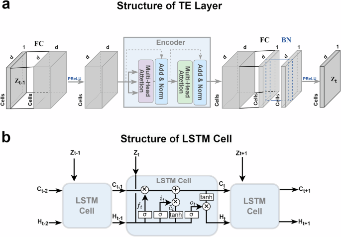
a A TE layer consists of fully-connected embedding layers combined with an Encoder module. b A standard LSTM cell contains an input gate i_t, a forget gate f_t, and an output gate o_t.

Full size image

Additionally, the sequential intermediate matrices Z_t serve as inputs to LSTM cells, which are a variant of RNNs specialized in handling sequences with long-range dependencies (see Fig. 2b). LSTM cells are employed to capture and characterize the sequential information in the outputs of the TE layers. The multiple outputs of the LSTM cells align with our multi-task framework. Specifically, the LSTM cell state C_T is used to predict the cell type through linear layers and softmax functions (Task 2), while the hidden embedding H_T serves as the low-dimensional representation of the cells. By using linear projection and the Uniform Manifold Approximation and Projection (UMAP) method³⁷, we can visualize the latent space of the datasets to demonstrate the effectiveness of data integration across different CITE-seq datasets (Task 3). Figure 1c, d detail the architecture of the scTEL model and the corresponding tasks.

Structure of TE layers and LSTM cells

Inspired by classical Transformer architecture, our TE layer employs the attention mechanism to extract key latent features in the spatial structure of data. The attention mechanism is the core of Transformer and may be the most exciting innovation in deep learning in the past few years. The attention mechanism is inspired by the mechanism of human vision that our eyes often focus limited attention on the important local areas rather than the whole scope. Thus, it can save computational resources and capture the essential information quickly. The self-attention mechanism in Vaswani et al. (2017)²⁶ is defined as follows:

where (Qin {{mathbb{R}}}^{dtimes d},Kin {{mathbb{R}}}^{dtimes d}), and (Vin {{mathbb{R}}}^{dtimes d}) are the query, key and value matrices respectively, which are outputs of three different linear layers with the same input. The dot product of Q and K^T measures the similarity between query and key. Then, the attention is calculated by the weighted average of the corresponding value V.

Furthermore, we concatenate multiple self-attention together, called multi-head attention, to improve the performance. Each attention function is executed in parallel with the respective projected versions of the query, key, and value matrices. The multi-head attention can be expressed as follows:

where i = 1, …, h and ({W}_{i}^{Q},{W}_{i}^{K},{W}_{i}^{V}) are weights of corresponding networks. The structure of the TE layer is shown in the Fig. 2a.

The sequential intermediate matrices Z_t serve as inputs to LSTM cells. The structure of the LSTM cell is shown in the Fig. 2b. Specifically, the feedforward steps in LSTM can be expressed as follows:

where C_t represents the cell state and H_t represents the hidden embedding. Here, W_f, W_i, W_o, W_c, and b_f, b_i, b_o, b_c, are weight matrices and bias vectors for the corresponding connection, σ(⋅) and tanh(⋅) represent the sigmoid function and the tanh function, [⋅ , ⋅] denotes the concat operation which merges the two vectors together, and ⊗ denotes the Hadamard product of two vectors.

Loss function

In deep learning, the choice of loss functions traditionally depends on the nature of the task. For regression problems, where the targets are continuous variables, mean squared error (MSE) is a commonly used loss function. For classification problems involving discrete target variables, cross-entropy loss is the standard choice. Our scTEL model encompasses multiple tasks, including protein expression prediction as a regression problem and cell type identification as a classification problem. Each task requires a suitable loss function to measure the discrepancy between the model’s predictions and the actual target values.

In Task 1, the scTEL model provides predictions for the expression matrix of reference proteins. Since the expression values are continuous, we consider using the MSE to measure the distance between the predicted expression matrix (hat{{bf{Y}}}={hat{{y}_{ij}}}) and the actual expression matrix Y = {y_ij}. Note that there are some empty entries in the true expression matrix due to the partial overlap of protein panels across different datasets. These empty entries are excluded from the loss calculation. Let B = {b_ij} be the indicator matrix with the same dimensions of Y, where b_ij = 1 if the expression value of j-th protein in the i-th cell is sequenced in CITE-seq datasets; otherwise b_ij = 0. Therefore, the MSE loss is defined as:

where n_train denotes the number of cells in the training set and p_ref denotes the number of reference proteins. Here, n_train and p_ref are the dimensions of the expression matrix of reference proteins Y.

Besides assessing the estimation error of the protein expression matrix, we also evaluate the uncertainty of the estimation by using the quantile loss function³⁸. Let Q = {q₁, q₂, ⋯ , q_M} be the set of quantiles we wish to estimate. The final output Z_T is projected through linear layers to independently generate the m-th quantile estimates ({{bf{Y}}}^{(m)}={{y}_{ij}^{(m)}}), for m = 1, 2, ⋯ , M. The quantile loss function is defined as:

where ({l}_{q}({y}_{ij},{y}_{ij}^{(m)})=[(1-{q}_{m})I({y}_{ij}^{(m)}, > ,{y}_{ij})+{q}_{m}I({y}_{ij}^{(m)} ,< ,{y}_{ij})]cdot | {y}_{ij}^{(m)}-{y}_{ij}|) denotes the entrywise quantile loss. Here, I(⋅) represents the indicator function, returning 1 if the inequality is true and 0 otherwise. This loss function evaluates the uncertainty of estimation and provides an overall view of the model’s performance.

In Task 2, which is a classification task, the scTEL model utilizes a linear layer coupled with a softmax function as the activation function on the final cell state C_T to output probability predictions for cell types, assuming the number of cell types is predefined. Each cell is then identified as the cell type with the highest prediction probability. For this multiple classification task, the categorical cross-entropy (CE) loss function is a common choice to measure the distance between the predicted and true distributions³⁹. Let ({boldsymbol{S}}=({s}_{1},{s}_{2},cdots ,,{s}_{{n}_{{rm{train}}}})) represent the true cell type labels for the cells in the training set. The CE loss function can be defined as:

where P_i(s_i) denotes the predicted probability that the i-th cell belongs to cell type s_i. This loss function focuses on maximizing the probability assigned to the correct class, thereby enhancing the model’s accuracy in cell type identification.

Finally, we aggregate the three loss functions as the total loss, which serves as the objective in the training process that needs to be minimized:

By calculating the gradient of the loss function with respect to the model’s parameters, the gradient descent algorithm can update the parameters in a direction that reduces the loss. The training loss is expected to converge to a lower level after sufficient epochs of iteration.

By minimizing the total loss, the scTEL model effectively captures the underlying connections between different tasks. It balances the objectives of each task and ensures that the trained model achieves optimal performance from a holistic perspective. For detailed information on the training process and model parameters, see the Supplementary Information.

In this section, we design three scenarios using four public CITE-seq datasets, including PBMC, MALT, H1N1, and Monocytes, to evaluate the performance of the scTEL model. We compare scTEL with traditional methods such as Seurat and totalVI, as well as the deep learning framework sciPENN. Our results demonstrate that the scTEL model significantly outperforms these existing approaches across all tasks.

Data integration and low-dimensional representation

In single-cell analysis, each cell is characterized by high-dimensional gene sequences. However, technical noise and samples from different sources can introduce batch effects, which may confound the biological interpretation of the data. Therefore, integrating multiple datasets and removing batch effects are essential steps for further analysis.

UMAP is a widely used method for visualizing batch effects by projecting the high-dimensional expression data into a low-dimensional space, typically 2D or 3D⁴⁰. After dimension reduction, each cell is plotted in the UMAP space and can be colored according to its batch label. This visual representation provides a clear indication of whether cells from different batches cluster separately (indicating batch effects) or intermingle (indicating successful mitigation of batch effects). Here, we explore three cases to evaluate the effectiveness of our scTEL model in data integration and batch effect correction by using UMAP visualization.

Case I: We divided the Monocytes dataset, which comprises 8 samples from 4 participants, into two subsets–Monocyte 1 and Monocyte 2, with each subset containing 4 samples from 2 participants. Since both subsets are sourced from the same laboratory and platform, the batch effect between the two subsets should be minimal. Figure 3a illustrates that most methods can integrate the two subsets well, with scTEL and sciPENN performing best by achieving complete data mixing. In contrast, totalVI shows some bias, and Seurat does not mix the subsets effectively.

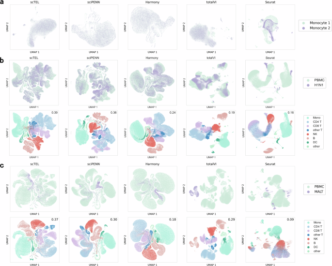
It demonstrates the effectiveness of data integration across three scenarios for the five compared models. The Silhouette score, shown in the top-right corner of each plot, provides a quantitative measure of clustering performance for the different models. a Case I, b Case II, c Case III.

Full size image

Case II: We consider integrating the PBMC and H1N1 datasets. Although sourced from different laboratories, the cell types in these two datasets are closely related. Specifically, the H1N1 dataset comprises human peripheral blood mononuclear cells infected with H1N1 influenza. The difference between the PBMC and H1N1 datasets is more pronounced than that in Case I. In this scenario, Fig. 3b demonstrates that scTEL significantly outperforms other methods by achieving completely mixed plots. In contrast, totalVI and Seurat fail to achieve sufficient mixing, resulting in the H1N1 data clustering separately.

Case III: We consider integrating the PBMC and MALT datasets, which are completely distinct with minimal featuring similarity. This scenario represents the most challenging integration task. Figure 3c shows that only scTEL is able to mix the datasets effectively, while in other methods, the MALT cells cluster separately, indicating poor integration performance. This highlights the superior ability of scTEL to handle and integrate highly disparate datasets.

To further assess the performance of each batch effect correction method and demonstrate that data integration avoids over-integration, we colored the true cell type labels in the PBMC and MALT datasets in Fig. 3b, c (note that true cell type labels are not available for the Monocytes dataset). Our results show that the two datasets are well-mixed in the scTEL model while maintaining clear and distinct clustering. Importantly, different clusters remain well-separated, indicating that the integration of the PBMC and MALT datasets avoids over-integration.

Furthermore, we employed the Silhouette score to quantitatively evaluate the clustering quality⁴¹. The results reveal that our scTEL model achieves the highest Silhouette scores across all cases, highlighting its superior performance.

From these cases, it is evident that as the difficulty of data integration increases, the scTEL model exhibits significant advantages over other methods. This demonstrates that scTEL can effectively handle data integration and mitigate batch effects, especially for highly disparate datasets.

Protein expression prediction

The primary goal of scTEL is to establish a mapping from RNA expression to protein expression. With a trained model, scTEL can impute the unsequenced protein expression in CITE-seq datasets, or predict a complete protein expression with scRNA-seq data (refer to Task 1 in Fig. 1d).

To evaluate the performance of models, both the root means square error (RMSE) and Pearson correlation are used to measure the distance between predicted and target expression levels for individual proteins within CITE-seq data²³:

where RMSE_j and ρ_j denote the RMSE and Pearson correlation between the predicted and target protein expression levels for the j-th protein, respectively. Here, ({mu }_{j}=frac{1}{mathop{sum }nolimits_{i = 1}^{{n}_{{rm{train}}}}{b}_{ij}}{b}_{ij}{y}_{ij}) and ({hat{mu }}_{j}=frac{1}{mathop{sum }nolimits_{i = 1}^{{n}_{{rm{train}}}}{b}_{ij}}{b}_{ij}{hat{y}}_{ij}) are sample mean of target and predicted expression levels.

Figure 4a illustrates the box plot of the RMSE for each protein across four models in three distinct settings as outlined in Section “Data Integration and Low-dimensional Representation”. Across all three settings, our scTEL model consistently exhibits the lowest average RMSE of all proteins. Especially in Case III, where PBMC and MALT datasets differ greatly, our scTEL model significantly outperforms other models.

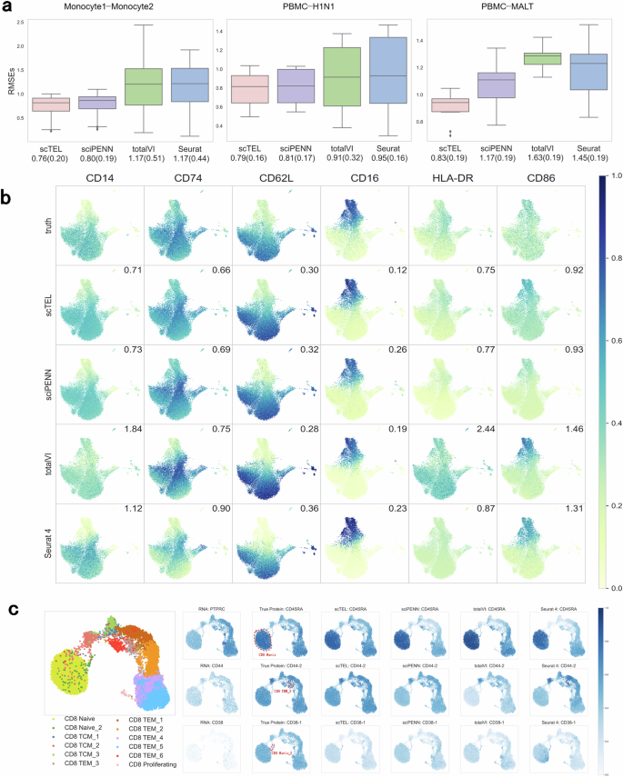
a Box plots of the RMSE for each protein across four models in three scenarios. The values at the bottom of the plot represent the means and standard errors of all proteins in each setting. b True and predicted expression levels of 6 overlapping marker proteins in Monocytes. The value indicated in the top-right corner of the plot corresponds to the RMSE for the specific protein in each setting. c The UMAP plot on the left illustrates the true labels of CD8 cell subpopulations in PBMC, while the UMAP plot on the right focuses on three specific subpopulations of CD8 cells: Naive, TEM3, and Naive2. By visualizing the expression patterns of marker proteins (CD45RA, CD44-2, and CD38-1) alongside their corresponding encoding RNA genes (PTPRC, CD44, and CD38), we demonstrate that protein expression predicted by scTEL enables the identification of specific cell subpopulations with high levels of particular protein expression.

Full size image

Figure 4b visualizes the expression levels of 7 overlapping marker proteins in Monocytes, including CD14, CD74, CD36, CD62L, CD16, HLA-DR, and CD86. These proteins play critical roles in the immune system, participating in pathogen recognition, regulation of immune responses, and various cell-cell interaction functions. In immunology, monocytes are classified into three subtypes–classical, non-classical, and intermediate–based on expression patterns of these proteins in immune cells^42,43. Compared with other models, scTEL provides the closest predictions to the true values. This demonstrates that our scTEL model performs effectively across different subtypes of monocytes.

Figure 4c shows the gene expression alongside the corresponding protein expressions in PBMC. Analyzing the expression of coding RNA genes alone is insufficient to distinguish cell subpopulations effectively. However, incorporating protein expression data helps address this limitation and provides a more comprehensive understanding. As an example, for the three subpopulations of CD8 cells: Naive, TEM3, and Naive2. Using UMAP, we visualize the expression of marker proteins (CD45RA, CD44-2, and CD38-1, respectively) and their corresponding encoding RNA genes (PTPRC, CD44, and CD38). The results demonstrate that protein expression predicted by scTEL allows researchers to identify the specific cell subpopulations where particular proteins are highly expressed.

Similarly, Fig. 5 presents the Pearson correlation between predicted and target expression values, with higher correlations indicating better model performance. Figure 5(a) illustrates the box plot of the correlation for each protein across four models. In all three settings, our scTEL model consistently exhibits the highest average Pearson correlation of all proteins. Figure 5b visualizes the expression levels of 10 marker proteins that are common to both PBMC and MALT datasets. Compared with other models, scTEL provides the highest correlation with the true values for all proteins.

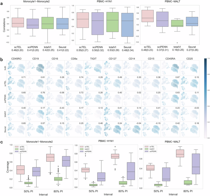
a Box plots of the Pearson correlation for each protein across four models in three scenarios. The values at the bottom of the plot represent the means and standard errors of all proteins in each setting. b True and predicted expression levels of 10 marker proteins that are common to both PBMC and MALT datasets. The value indicated in the top-right corner of the plot corresponds to the correlation for the specific protein in each setting. c Box plots of coverage probabilities for proteins under 50% PI and 80% PI for the three models.

Full size image

To consider the uncertainty of model predictions, we calculate the coverage probability, which indicates the proportion of true values that fall within the prediction intervals (PI), for individual proteins. A higher coverage probability reflects greater robustness of the models. As Seurat does not quantify protein expression prediction uncertainty, our comparison is limited to sciPENN and totalVI. Figure 5c depicts the box plot of coverage probabilities for proteins under 50% PI and 80% PI for the three models. Our scTEL model consistently outperforms the others in all scenarios. Table 2 provides a summary of the median coverage probability in each setting. As the task difficulty increases (from Case I to Case III), scTEL maintains robust performance, with the median coverage probability remaining stable across all settings. In contrast, sciPENN and totalVI experience a significant decline in performance, particularly in the more challenging Cases II and III.

Cell type identification

Cell type identification and annotation constitute another critical aspect of single-cell analysis. Traditional scRNA-seq data analysis typically employ dimension reduction and clustering techniques on RNA expression matrices, followed by the identification of cell types using marker genes. However, certain cell types may not be easily distinguished based solely on RNA expression, particularly for some rare subtypes. Accurately distinguishing these cell subtypes is essential for capturing cellular heterogeneity and understanding the diverse functions within biological systems^44,45.

Our scTEL offers a powerful tool for identifying cell types, leveraging both RNA and protein expression data to enhance classification accuracy. In this section, we assess the performance of our model in cell type identification using PBMC datasets. TotalVI is excluded from the model comparison, as it is not designed for cell type identification. Hao et al. (2021)²⁸ provides high-resolution labels with 57 categories for PBMC datasets, encompassing all major and minor immune cell types. Our task is a multi-classification task that classifies observed cells into 57 categories, which poses a challenge since the subtypes may exhibit similar expression patterns. Figure 6a present the confusion matrix, where the rows represent the true cell types and the columns represent the predicted cell types. Overall, scTEL achieves a significantly higher accuracy of 86.6% in cell type classification, outperforming sciPENN (77.0%) and Seurat (76.1%). Additionally, we assessed the classification performance using the F1-score and Adjusted Rand Index (ARI)⁴⁶, as shown in Fig. 6a. The results consistently indicate that our scTEL model surpasses existing approaches across all evaluation metrics.

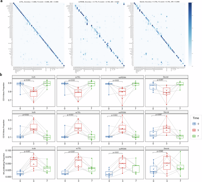
a The heatmap of the confusion matrix visualizes the classification performance, where the rows represent the true cell types and the columns represent the predicted cell types. All the three assessment metrics (accuracy, F1-score, and ARI) demonstrate that our scTEL model outperforms existing approaches. b The variation in the proportion of CD14 monocytes, CD16 monocytes, and NK proliferating at 3 time points in seven donors. The p values are reported from a paired Wilcoxon signed-rank test to compare the proportions of cells before vaccination and 3 days after vaccination.

Full size image

Moreover, donors in the PBMC dataset received a vesicular stomatitis virus (VSV)-vectored HIV vaccine. Cell expression profiles were collected from patients at 3 time points: immediately before the vaccine, 3 days after the vaccine, and then 7 days after the vaccine. Hao et al. (2021)²⁸ reported that CD14 monocytes, CD16 monocytes, and NK proliferating exhibit distinct responses to the vaccine. Figure 6b illustrates the variation in the proportion of these three subtypes at different time points. Our scTEL model provides the closest predictions to the true pattern compared with sciPENN and Seurat.

Life is a complex system. In modern molecular biology, according to the central dogma, genetic information is transcribed into RNA and then translated into proteins, which play a central role in shaping the diverse functions of cells and organisms. However, due to limitations in techniques and the high costs associated with experiments, research on proteomics is often challenging and constrained. These limitations hinder our comprehensive understanding of life activity as a whole.

In this paper, we propose an integrated framework, scTEL, to model RNA and protein expression jointly at the single-cell level. Leveraging CITE-seq datasets, our scTEL model establishes a mapping from sequenced RNA expression to the unobserved protein expression within the same cells. This advancement enables the prediction of protein expression using scRNA-seq data at a lower cost. In a unified framework, we achieve data integration, protein expression prediction, and cell type identification, forming a complete workflow for single-cell analysis. Through empirical validation on public datasets, we demonstrate that scTEL significantly outperforms traditional methods such as Seurat or totalVI in various tasks. Moreover, it exhibits superior performance compared to the RNN-based model sciPENN. The architecture of Transformer encoding layers and LSTM cells in scTEL significantly contributes to feature extraction in multi-omics data analysis.

In practice, scTEL still has several limitations. First, its sophisticated deep learning framework requires high computational resources, especially when handling large-scale single-cell datasets. Striking a balance between model performance and computational costs remains a challenging issue. Second, the training of the scTEL model relies on the access to reliable and well-annotated single-cell datasets, such as PBMC, which may limit its broader applicability.

Nowadays, integrated analysis of multi-omics data is becoming increasingly essential in cell biological research. It is crucial to analyze various related data types together to gain a comprehensive understanding of cellular processes. In the future work, we will consider to incorporate additional omics data, such as metabolomics and epigenetics, into our analysis framework.