A mathematical framework for comparison of intermittent versus continuous adaptive chemotherapy dosing in cancer

Introduction
Thanks to advances in medicine and cancer treatments, more and more patients are living longer with metastatic cancer1,2. In these patients, a cure is often not possible and the goal is to limit overall side effects from cancer treatments, prolong progression-free survival, and limit symptoms from the cancer itself3.
Chemotherapy dosing has traditionally derived from the maximum tolerated dose (MTD) principle4 (Fig. 1). For chemotherapy or combination chemotherapy that is associated with high levels of toxicity for patients, dosing is often based on how often the chemotherapy can be given without incurring severe side effects as measured in clinical trials. The final dosing schedule is typically fixed (every 2 weeks, every 3 weeks, etc.) as is the number of doses that a patient ultimately receives (termed “cycles”). The dosing schedule can be adjusted based on patient status (e.g. dosing may be delayed if a patient becomes sick) or discontinued if the patient’s tumor is not responding to treatment. As an alternative to MTD, metronomic dosing, where a chemotherapy is administered at a lower dose and given at regular intervals, has been utilized to minimize toxicity and control disease progression5,6. For certain chemotherapeutic agents that are relatively non-toxic and available in oral formulation, dosing may be given daily as tolerated to achieve a stable steady state concentration of drug in the body (continuous fixed-dose therapy). This type of treatment can be considered metronomic therapy and is used clinically alone or in combination with other chemotherapeutic agents and dosing strategies7. Ultimately, many advanced metastatic cancers progress through standard treatment and become refractory to chemotherapy.

Cytotoxic chemotherapy at maximum tolerated dose (MTD) results in early extinction of the sensitive cell population. Two adaptive therapy models are shown: intermittent adaptive therapy (resulting from on-off dose modulation aka “dose-skipping”) and continuous adaptive therapy (resulting from dose modulation to maintain a given tumor volume). Finally, fixed low dose therapy in the antiproliferative range of drug action is shown and is considered a type of metronomic therapy. Created with Biorender.com.
In broad terms, a tumor is defined as sensitive to a given chemotherapy if it shrinks or does not grow with treatment. A tumor is defined as resistant to chemotherapy if it continues to grow in the presence of treatment. While these terms are applied to entire tumors, in reality, tumors are heterogeneous and may contain subpopulations of drug resistant and sensitive cells. Pan-cancer analysis of intratumoral tumor heterogeneity has suggested that high heterogeneity is correlated with decreased overall survival across a variety of cancer types8. The mechanisms by which interactions between these subpopulations contribute to treatment response and resistance is likely highly dependent on the type of cancer, the tumor microenvironment and architecture, and the resistance mechanism in question.
The concept of controlling disease evolution and resistance through drug treatment has been an area of interest in oncology and infectious disease9. Adaptive chemotherapy administration, wherein a drug schedule or dose is dependent on tumor size (or some other metric of tumor burden), has been proposed as a method to lengthen progression-free survival in cancers where a resistant subpopulation already present in the tumor is likely to drive disease progression10,11,12. This method has shown some success in increasing progression-free survival in a clinical trial of patients with advanced metastatic prostate cancer12 and in preclinical models of ovarian cancer, breast cancer, and melanoma10,13,14. There are planned and ongoing clinical trials to evaluate adaptive strategies in the treatment of rhabdomyosarcoma, prostate cancer, melanoma, ovarian cancer, and advanced basal cell carcinoma15.
The rationale for implementation of adaptive therapy is based largely on two ecological principles: fitness cost and competitive release. In the context of cancer cell competition, fitness cost is the idea that becoming chemotherapy resistant inherently leads to a trade-off in some other area of ecological fitness10. The observation that slower growth rates of cancer cell subpopulations can lead to chemoresistance to traditional cytotoxic chemotherapy16 can be used as evidence of this cost. Additionally, resistant cell upregulation of drug efflux pumps which consume large amounts of cellular ATP17 is a plausible mechanism by which a fitness cost to resistance is incurred for certain drugs. However, whether or not fitness cost in the context of slower growth of chemoresistant cells or other mechanisms applies more widely across newer targeted inhibitor therapies remains to be seen. Recent exploration of adaptive therapy models suggests that even without significant differences in growth rate between sensitive and resistant cells, there is still a progression-free survival advantage with adaptive therapy over traditional fixed dosing schemes18.
The observation of continued efficacy of adaptive chemotherapy even without a fitness cost of resistance derives from the ecological principle of competitive release. Assuming individual cancer cells are competing for resources (space, blood flow, nutrients, etc.), then the ability of cells to proliferate is dependent upon the overall density of cells. Thus, the closer a tumor is to its carrying capacity (the number of tumor cells that can be sustained by the local environment), the lower the growth rate of the tumor. In traditional dosing schemes, the goal of treatment is to maximally shrink the tumor which results in rapid reduction of the drug sensitive species and thus tumor volume. With this reduction in overall tumor volume, the resistant cells are able to proliferate faster. The observed rapid proliferation of the resistant cells is termed competitive release. Under adaptive dosing strategies, however, the sensitive cell population is purposefully maintained within the tumor in order to inhibit competitive release of the resistant cell population10,11,12.
Adaptive therapy strategies can be broadly categorized as intermittent or continuous. In intermittent adaptive therapy, a fixed-dose of drug is given until a tumor reaches a certain lower size threshold and then withdrawn until the tumor regrows to a certain upper size threshold (Fig. 1). This has also been coined “on-off” adaptive therapy or “dose-skipping” adaptive therapy15. In continuous adaptive therapy, on the other hand, a drug is given with variable dosing to hold a tumor to a given volume, also termed “dose modulation” adaptive therapy15 (Fig. 1). Continuous adaptive therapy can be implemented through sequential dose changes with the goal to hold tumor volume constant. Algorithms for these dose changes have been studied in vivo in mouse models13. Similar to intermittent adaptive therapy, continuous adaptive therapy requires monitoring of tumor volume for dose adjustments. Conceptually, this is most easily achievable with drugs available in oral formulation which reach steady-state concentrations based on daily dosing. This can also be achieved with intravenous medications through the use of continuous infusion pumps. Direct comparison between intermittent adaptive therapy and continuous adaptive therapy has been explored experimentally13 and computationally19 in an agent based model. Mathematically, the observation that higher tumor volume implies slower growth has demonstrated that continuous adaptive therapy held at the highest tolerated tumor volume maximizes time to treatment failure and may be superior to intermittent adaptive therapy20. However, formal mathematical analysis of intermittent adaptive therapy has been limited due to the discontinuous nature of the dosing function.
In this work, we show that intermittent adaptive therapy can be mathematically modeled as a bang-bang control problem21 and that, under certain conditions, the resistant population can be driven to extinction. We prove that the analytical limit as the upper and lower control boundaries of adaptive therapy approach each other yields a continuous dosing function and that this continuous dosing function is equivalent to continuous adaptive therapy. Using this result, we show that continuous adaptive therapy maximizes time to resistant subpopulation outgrowth (disease progression) relative to intermittent adaptive therapy.
In the case where the resistant population can be driven to extinction, we show that when compared to intermittent adaptive therapy, continuous adaptive therapy is more robust to uncertainty in initial conditions, yields a quicker time to resistant population eradication, and carries the lowest cumulative toxicity. Finally, we show that the continuous dosing function is in the antiproliferative range of drug action and thus can be directly compared with fixed low-dose continuous therapy, a type of metronomic therapy (Fig. 1). An unexpected advantage of this continuous metronomic therapy over adaptive therapy is that it can result in resistant extinction under an often broader set of initial conditions than adaptive therapy. Furthermore, fixed-dose therapy is biologically and clinically easier to implement. To our knowledge, this is the first direct analytical comparison between continuous and intermittent adaptive therapy dosing regimes in cancer and demonstrates the utility of this benchmarking approach to compare continuous control models with bang-bang control models for understanding tumor evolution under drug perturbation.
Results
Mathematical model
The Lotka-Volterra equations are a well established dynamical system for studying competition between species22. For the purposes of this manuscript, the two species Lotka-Volterra model is described below for the sensitive cell population, x, and the resistant cell population, y, under logistic growth with carrying capacity of each species normalized to 1. A conceptual representation of this model is shown in Fig. 2A.
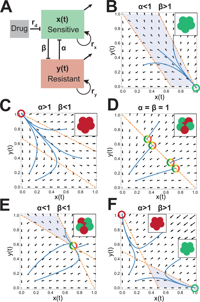
A Conceptual representation of cell-cell competition model. The growth rates of the sensitive and resistant populations are given by rx and ry respectively. α and β are the competition parameters of y on x and x on y respectively. The carrying capacity of each species is normalized to 1. Drug dose is given by rd and acts only to decrease the sensitive species. B–F Vector fields corresponding to different relative competition strengths between the sensitive and resistant cell populations without drug. The nullclines are plotted in orange. The equilibrium states are shown as illustrations in the upper right insets and areas where ({x}^{{prime} } > 0) and ({y}^{{prime} } < 0) are shaded blue.
The major difference between this model and a traditional competition model is the presence of a treatment indicator function KA(x, y, t) in Equation (1) which takes values 1 or 0 depending on whether the drug is on or off respectively. The effect of the drug on the sensitive cell line is given by the function h(x, rd) where rd is the “dose” of drug.
Drug effect in this paper is modeled as removal of the sensitive cell population and is assumed to be a linear process as shown:
Representing drug action in this manner allows for a range of drug effect from antiproliferative (decreasing the growth rate of the sensitive cells) to cytotoxic (leading to sensitive cell extinction) based on administered dose. (See Supplemental Figure S2 and Supplemental Section 1.3).
The behavior of this model in the absence of drug is shown in Fig. 2B–F. Note that when the sensitive or resistant cell line is a strong competitor (α or β > 1 respectively) relative to weak competition (β or α < 1) from the other subpopulation, the equilibrium state is composed of the single stronger species at carrying capacity while the weaker subpopulation is driven to extinction (Fig. 2B, C). On the other hand, when both are weak competitors (2E) an equilibrium heterogeneous state exists; and when both are strong competitors (2F) the tumors trend to homogeneous populations determined by the initial conditions. Finally, if competition terms are both equal to 1, the heterogeneous tumor is stable with the subpopulation ratio dependent on initial conditions. Note that the growth rate (given by rx and ry) for each species does not affect the position of the nullclines in this model.
Importantly, if the goal of treatment is to reduce the resistant population to near 0, then the natural strategy is not to treat in parameter spaces in which the system equilibrium at carrying capacity results in an entirely sensitive tumor. This seemingly paradoxical statement derives from the equilibrium state shown in Fig. 2B and underscores the importance of defining the optimization problem as maintaining the total tumor volume less than carrying capacity. Therefore, we assume that the maximal tumor size (sensitive plus resistant cells) must be maintained at a volume less than carrying capacity and we call this the upper control line, A.
Intermittent adaptive therapy
Intermittent adaptive therapy is modeled using bang-bang control where the controller is turned on (KA = 1) when the total tumor volume (resistant + sensitive) reaches the upper control line, x + y = A. Once the tumor volume has decreased to the lower control line, A − δ, where δ is chosen to be a value less than A, the controller is turned off (KA = 0) and the tumor regrows. Of note, this model is not a classical optimal control problem as the control parameter KA takes the values of 0 and 1 only and there is no running cost for which we are seeking optimization.
In clinical implementations of adaptive therapy, A − δ is chosen as a clinically detectable decrease in tumor size. For example, decrease in serum prostate specific antigen (PSA) by 50% (in this formulation (delta =frac{A}{2})) was chosen in the recent Phase 1B clinical trial in prostate cancer as a biomarker for tumor size reduction by 50%23. During the tumor size reduction phase (KA = 1) the dose of drug is held constant at rd which is assumed to be in the cytotoxic range. The flipping strategy is continued indefinitely or until the tumor is no longer controllable (e.g. the tumor size cannot be decreased to A − δ with administration of fixed-dose drug, rd).
In the case where the resistant cell population is a weaker competitor than the sensitive cell population (α < 1 and β > 1, Fig. 2B), the relative position between the upper and lower control lines and the y-nullcline yields the possibility of three distinct behaviors that are dependent on the initial tumor composition. Figure 3 shows an example phase space (Fig. 3A) and trajectories under varying initial conditions demonstrating sensitive cell population extinction (Fig. 3B) sensitive/resistant equilibrium (Fig. 3C), and extinction of the resistant cell population (Fig. 3D).
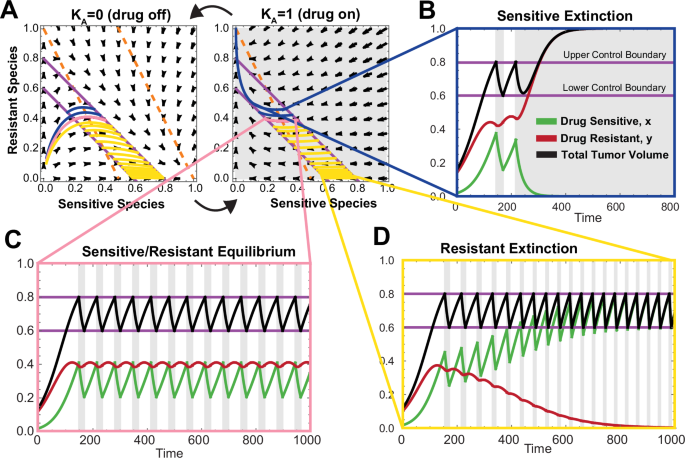
A Phase space for drug on and drug off with 3 trajectories of adaptive therapy plotted (light blue, pink, and dark blue) under the same simulation parameters with different initial conditions. Nullclines are shown as dashed orange lines. B Sensitive extinction time course corresponding to the dark blue trajectory in phase space shown in (A). C Sensitive/resistant equilibrium time course corresponding to the pink trajectory in phase plane shown in (A). D Resistant extinction time course corresponding to the light blue trajectory in phase space shown in (A).
The case where the resistant cell population is the stronger competitor yields only one outcome (sensitive extinction) and is shown in Supplemental Figure S4 and discussed in Supplemental Section 2.1.2. In this case, while resistant extinction is not achievable, intermittent adaptive therapy lengthens time to tumor progression over continuous treatment with the same dose of drug or no treatment. This result is consistent with previously reported work using similar a model18.
Optimal intermittent adaptive therapy converges to continuous adaptive therapy
In this model, the higher the total cell population, the lower the resistant population growth rate. Thus decreasing δ with a fixed upper tumor volume intuitively increases the time to resistant population outgrowth under conditions fated for sensitive cell population extinction. Similarly, under conditions leading to resistant cell population extinction, decreasing δ decreases time to resistant extinction. With this intuition in mind, we formally explore the analytical limit of adaptive therapy as δ → 0 for fixed upper control line x + y = A. See Supplemental Sections 2.2–2.5 for mathematical discussion.
We prove that intermittent adaptive therapy converges to the x + y = A line in the δ → 0 limit (Supplemental Theorem 2.7) within a formally defined control region in phase space (Supplemental Section 2.3). We similarly define the strict control region to be the portion of phase space where the the limit as δ → 0 of intermittent adaptive therapy is always in control and the tumor volume never increases above A (Supplemental Definition 2.3).
A simulation of this limiting system is shown in Fig. 4C. Note that the limiting trajectory as δ → 0 recapitulates the behavior of the oscillating system shown in Fig. 3. At the point of intersection between the control line and the y-nullcline, an unstable equilibrium exists corresponding to the equilibrium seen in Fig. 3C. Similarly, resistant extinction and sensitive extinction are determined based on the intersection of the initial trajectory with the x + y = A line.
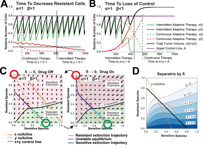
A Time to decrease resistant cell population to threshold (y = 0.01) when α < 1 and β > 1 under intermittent adaptive therapy (solid lines) and continuous adaptive therapy (dotted lines). (Model Parameters: α = 0.5, β = 2, rd = 0.1, rx = 0.03, ry = 0.02, A = 0.8., δ = 0.4) B Time to loss of control when α > 1 and β < 1 under intermittent adaptive therapy (solid lines) and continuous adaptive therapy (dotted lines). (Model Parameters: α = 1.5, β = 0.7, rd = 0.1, rx = 0.03, ry = 0.02, A = 0.8., δ = 0.4) C Phase planes corresponding to δ → 0 trajectories with the numerically computed separatrix delineating between initial conditions leading to resistant species extinction and those leading to sensitive species extinction. D Numerically computed separatrix for varying values of δ (Model Parameters: α = 0.5, β = 2, rd = 0.05, rx = 0.03, ry = 0.02). Theoretical computation of the separatrix is discussed in Supplemental Section 2.4 and has excellent concordance with numerical results.
The observation that intermittent adaptive therapy converges in the limit as δ → 0 can be used to compute a continuous dosing function that holds the tumor volume constant at A in the control region (Supplemental Equation 30). This continuous dosing function is a smooth function essentially representing a time averaged rd and is equivalent to continuous adaptive therapy (dose modulation) on the x + y = A line by definition. The continuous dosing function, ({hat{R}}_{c}(x)), is a function of the sensitive cell population, x, and its shape depends on the underlying phase space. In certain cases, ({hat{R}}_{c}(x)) represents a decreasing function consistent with reported experimental observations13 (Supplemental Fig. S12). When resistant extinction can be achieved, this function takes values in the anti-proliferative range of drug action (Supplemental Corollary 2.6). Interestingly, the dosing function ({hat{R}}_{c}(x)) does not depend on the original intermittent adaptive therapy dose, suggesting that it represents an absolute theoretical limit independent of rd. Importantly, while mathematically equivalent to continuous adaptive therapy, this functional form does not provide specific insight into experimental implementation of continuous adaptive therapy as the dose is calculated based on the number of sensitive cells. When implemented, continuous adaptive therapy, like intermittent adaptive therapy, relies on ongoing measurements of total tumor volume to modulate the drug dose rather than a subpopulation of cells within the tumor13.
The knowledge that intermittent adaptive therapy converges to continuous adaptive therapy as δ decreases allows for formal comparison of these two adaptive therapy modalities. We show that the limit of time to disease control or loss of control as δ → 0 in intermittent adaptive therapy converges to the computed time in continuous adaptive therapy. This allows us to show that the time to loss of control is larger under continuous adaptive therapy than under intermittent adaptive therapy (Supplemental Section 2.6). Similarly, the time to resistant extinction (when possible) is smaller under continuous adaptive therapy (Supplemental Section 2.6 and Figure S8A). Example simulations of these results are shown in Fig. 4A, B.
Drug toxicity, which can result in unwanted side effects and decreased quality of life, is an important parameter for minimization in comparing treatment modalities and derives from the cumulative time undergoing treatment in a dose-toxicity relationship. Interestingly, unlike time, cumulative drug toxicity does not always converge. We show that when cumulative drug toxicity is modeled as an increasing nonlinear function of drug dose, drug toxicity as δ → 0 is strictly larger under intermittent adaptive therapy than continuous adaptive therapy under mild conditions on the toxicity function (See Supplemental Section 2.7 and Figure S8B). This result underscores the importance of analytic comparison between these two modalities and demonstrates that drug toxicity may be significantly different between intermittent and continuous adaptive therapy. It further suggests an absolute advantage of continuous adaptive therapy over optimal intermittent adaptive therapy.
Finally, in addition to drug toxicity, one of the most important aspects of a therapeutic strategy is robustness to uncertainty in parameters. Specifically, the relative composition of a tumor in terms of sensitive versus resistant subpopulations may be difficult, if not impossible, to attain precisely. We note that as δ decreases, the parameter space of tumor compositions that lead to resistant population extinction increases (See Fig. 4D). Mathematically, it is shown that the strict control region for continuous adaptive therapy is strictly greater than the strict control region for intermittent adaptive therapy (See Supplemental Section 2.4). This suggests a further advantage of continuous adaptive therapy over intermittent adaptive therapy in cases where resistant extinction is possible.
Continuous fixed-dose treatment is non-inferior to intermittent and continuous adaptive therapy for resistant population extinction
In the previous section, we showed that in regions where resistant subpopulation extinction is possible, continuous adaptive therapy is superior to intermittent adaptive therapy in minimization of the time to resistant population extinction, minimization of overall drug toxicity, and maximization of initial conditions leading to resistant subpopulation extinction. As resistant subpopulation extinction yields the possibility of total tumor eradication, it presents an enticing area for further analysis. Accordingly, we sought to further characterize this region to understand the relative benefits and limitations of adaptive therapy versus standard fixed-dose therapies.
Analysis of this model under continuous fixed-dose drug administration again demonstrates that continuous cytotoxic doses of chemotherapy lead to rapid release of resistant cells and tumor outgrowth (Fig. 5B). Anti-proliferative drug doses (rd < rx), on the other hand, act to decrease the sensitive species carrying capacity and slow their growth rate in the absence of a competing resistant cell line (Fig. 5A and C and Supplemental Section 1.3). Similar to the results shown for adaptive therapy, fixed continuous doses of anti-proliferative drug can be identified that maintain the sensitive cell population indefinitely and lead to extinction of the resistant cell population. Interestingly, when a weakly competitive resistant cell population competes with the sensitive one, the same anti-proliferative dose of drug that results in sensitive cell population maintenance in the absence of competition may become “effectively cytotoxic” and trigger extinction of the sensitive cell population (Fig. 5B, Supplemental Figure S10, and Supplemental Section 3.1). This result has implications beyond adaptive therapy. Specifically, drugs that are measured to be anti-proliferative in vitro or under conditions where nutrients and space are not growth limiting may be effectively cytotoxic in more realistic tumor environments where growth is constrained by the surrounding tissue and a competing normal cell population. Finally, in the case where the resistant cells are strong competitors, resistant cell population extinction is not achievable under continuous fixed-dose therapy. Here, lower doses of drug result in increasing times to resistant cell population outgrowth (Supplemental Section 3.1).
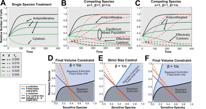
A Treatment of the single species sensitive cell population alone versus (B) treatment with the same doses of drug (rd) in a mix of sensitive and resistant competing cells when β < 1/α and (C) when β > 1/α. D Phase plane when (beta < frac{1}{alpha }) with the continuous adaptive δ = 0 separatrix shown in black with initial conditions under the line leading to resistant extinction (shaded grey). All initial conditions lead to resistant extinction under fixed-dose continuous therapy (shaded blue) with the minimum achievable tumor volume taken when rd is set such that the intersection of the x and y nullclines occurs on the x-axis. E Phase planes when (beta > frac{1}{alpha }) with the continuous adaptive δ = 0 separatrix shown in black with initial conditions under the line leading to resistant extinction (shaded grey). In the first phase plane, rd is chosen such that for all initial conditions where continuous adaptive control leads to resistant population extinction, continuous fixed-dose treatment will also yield resistant species extinction with final tumor size smaller than A. F In the second phase plane, rd is set such that the equilibrium under fixed-dose control for favorable initial conditions (shaded blue) is set to A. Simulation Parameters: (A–C), rx = 0.04, ry = 0.03, (x0, y0) = (0.3, 0.1) except (A) where y0 = 0. In (B), α = 0.5 and β = 1.5. In (C), α = 0.9 and β = 2.
In cases where resistant subpopulation extinction is achievable under both continuous fixed-dose therapy and continuous adaptive therapy, we analyzed the minimum tumor volume at which the tumor could be maintained. This is divided into two cases. When β < 1/α, this minimum volume is explicitly solvable (see Supplemental Section 3.2) and is shown to be the minimum tumor volume by phase plane argument. Knowing this minimum tumor volume allows us to calculate the drug dose rd needed to achieve control at the minimum achievable volume (See Supplemental Proposition 3.1) under any initial tumor composition. Continuous adaptive therapy, on the other hand, results in resistant species extinction only under certain initial conditions. Therefore, it is less robust to uncertainty in initial conditions than continuous fixed-dose therapy (Fig. 5C). It is important to note that in the regions where continuous fixed-dose therapy can result in resistant population extinction and adaptive therapy cannot, the tumor size must increase above the upper tumor control volume, A, for a period of time even though steady-state maintenance of tumor volume will be at or below A. An unexpected result of this analysis is that the optimal strategy to minimize the size of tumor outgrowth above A is to wait to initiate continuous fixed-dose treatment until the tumor volume reaches A.
For the second case when β > 1/α, a different minimum achievable tumor volume is given under continuous fixed-dose therapy and there is a dependence on initial conditions. However, the space of initial conditions leading to resistant extinction is always greater than or equal to that in continuous adaptive therapy for the same final tumor volume constraint (Fig. 5D and Supplemental Section 3.3). Furthermore, there are a set of initial conditions under which resistant species extinction can be achieved under fixed-dose therapy but not adaptive therapy. Again, the tumor volume in these cases may increase above A transiently and this increase can be minimized by initiating treatment when the tumor size reaches A.
There are clinical examples of delayed treatment paradigms in cancer. Specifically, delay in androgen deprivation treatment (ADT) initiation after biochemical recurrence of prostate cancer (detectable PSA) in low-risk patients is generally the preferred clinical approach due to toxicities associated with ADT and lack of clear clinical benefit in low risk patients24,25,26,27. Similarly, in early stage asymptomatic chronic lymphocytic leukemia (CLL) treatment delay is the standard of care due to lack of clinical benefit and toxicity associated with treatment initiation28,29. The above mathematical analysis suggests that in specific cases where cell-cell competition can be harnessed to drive the resistant population extinct, delayed treatment could theoretically minimize maximum tumor size.
In summary, direct comparison of continuous adaptive therapy versus continuous fixed-dose therapy demonstrates that both strategies may lead to resistant extinction under certain conditions and that the set of initial conditions leading to resistant species extinction under fixed-dose therapy is broader than those under adaptive therapy. In cases where resistant control is not possible under adaptive therapy but is possible with continuous fixed-dose therapy, the tumor size will exceed the upper control line for a period of time to achieve resistant species extinction. This effect is minimized if the treatment is initiated once tumor volume reaches the upper control line. Taken together, we conclude that continuous fixed-dose therapy is mathematically non-inferior to continuous adaptive therapy in achieving resistant species extinction and that if tumor volume need not be strictly controlled, then continuous fixed-dose therapy may be superior. Given the practical considerations of ease of dosing for fixed-dose therapy, this strategy may be preferable in practice.
Discussion
In this study, a modified Lotka-Volterra model of adaptive therapy is described that can be used to analytically examine intermittent adaptive therapy as a bang-bang control problem. It is shown that as the lower dosing threshold approaches the upper control line, the limit of this intermittent dosing converges to the upper control line and has equivalent behavior to continuous adaptive therapy. In cases where resistant population control is not achievable, continuous adaptive therapy is superior to intermittent cytotoxic dosing in delaying resistant cell population outgrowth. These results are consistent with results put forward by Viossat et al.20 but differ in their theoretical connotation. Specifically, it is proven that intermittent adaptive therapy is equivalent to continuous adaptive therapy in the limit irrespective of the given fixed intermittent dose and that continuous adaptive therapy provides an upper boundary to idealized intermittent adaptive therapy behavior. We further prove that cumulative drug toxicity is strictly lower in continuous adaptive therapy over intermittent adaptive therapy, suggesting an absolute clinical advantage of this treatment modality.
We additionally define a set of initial conditions for which resistant population extinction is achievable when the sensitive cell line is a stronger competitor than the resistant cell line (“fitness cost”). We show that for these conditions, continuous adaptive therapy is superior to intermittent adaptive therapy in terms of the time to resistant population extinction, cumulative drug toxicity, and robustness to uncertainty in initial conditions (Fig. 6). While adaptive therapy clearly outperforms cytotoxic continuous fixed-dose therapy, continuous antiproliferative fixed-dose therapy, a type of metronomic therapy, offers increased robustness to uncertainty in initial conditions over adaptive therapy provided that tumor size need not be strictly contained for the entirety of treatment (Fig. 6). We therefore conclude that in this region, continuous fixed-dose therapy is mathematically non-inferior to continuous adaptive therapy. As metronomic dosing is well established in practice and clinically requires less frequent monitoring, the practical considerations likely favor this therapy over continuous adaptive therapy.
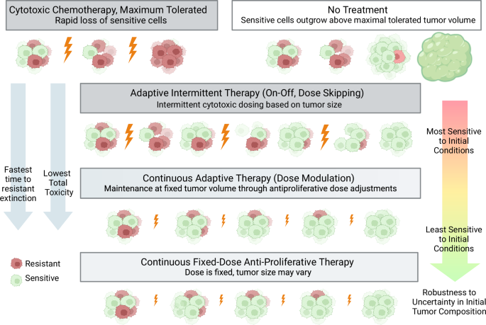
Under the three treatment regimens discussed in this work (adaptive intermittent therapy, continuous adaptive therapy, and continuous fixed-dose therapy), the sensitive cell population is maintained to slow resistant growth through competition. Continuous adaptive therapy demonstrates the fastest time to resistant extinction and the lowest total toxicity of the adaptive therapy paradigms. Consistent with phase plane arguments outlined in Fig. 5, continuous fixed-dose therapy can result in resistant extinction under the widest set of initial conditions, making it the most robust to uncertainty in tumor composition.Created with Biorender.com.
Exploration of the space where resistant species extinction is possible has been previously limited as it necessitates strong competition from the sensitive cell line and maintenance at a tumor volume that is high relative to the overall carrying capacity20. However, it is possible that combination therapy targeted at weakening the competitiveness of the resistant cell line and/or modulating the carrying capacity of the space may create circumstances where therapy aimed at extinction of the resistant cell population could be employed. As extinction of the resistant cell population creates the opportunity for tumor eradication at the end of therapy, it represents an important and enticing area for formal analysis.
This study is intended to provide a conceptual mathematical framework for comparing intermittent and continuous adaptive therapy against standard dosing regimes including MTD and continuous metronomic therapy in cases where competition between sensitive and resistant cell population drive resistance development. The presented work is purely mathematical in nature and limited by a lack of in vitro or in vivo data to validate the model of drug action, cell competition, and logistic growth. This model does not take into account spatial heterogeneity and assumes that populations of cells are well mixed. This model also assumes all resistance is pre-existing and does not account for accumulation of mutations (either drug induced or inherent) during therapy which can be modeled using a variety of approaches30,31,32. Additionally, drug induced chemotherapy resistance through non-genetic mechanisms is not accounted for in this model and may have important implications for optimal mathematical treatment strategies33,34,35,36. Despite the above limitations, we note that adaptive therapy competition models similar to the one presented in this work have formed the basis for ongoing computational and experimental studies in adaptive therapy and therefore represent an important class of models meriting formal mathematical analysis10,11,12,15,18.
In addition to the limitations of this particular model, it is important to note that the implementation of adaptive therapy itself is limited by biological and technical considerations. For example, if a resistant subpopulation of cells does not exist within a tumor, there is no benefit to adaptive therapy and the implementation of this strategy may lead to the accumulation of additional mutations as well as potential clinical morbidity. Adaptive therapy strategies are additionally limited by the ability to accurately track tumor volume in time. Initial clinical trials have been performed in prostate cancer with the biomarker PSA as a proxy for tumor volume12, however, it is unclear how best to track tumor volume in other tumor types where biomarkers corresponding to tumor size are not readily available. Tracking tumor volumes additionally makes the administration of continuous adaptive therapy potentially as difficult as intermittent adaptive therapy due to the need for a measurable increase or decrease in tumor volume in order to inform dose adjustments. These considerations are ameliorated somewhat by continuous fixed-dose therapy, however, choosing the correct initial dose depends on knowledge of tumor parameters which may not be feasible to attain. These considerations have been addressed in recent work aimed at drug titration algorithms to determine stabilization doses of chemotherapy20,37,38.
Despite the above limitations, several unexpected theoretical advantages of adaptive therapy exist including the observation by Enriquez-Navas et al. that adaptive therapy schemes may maintain or increase tumor vascularity in preclinical models13. While it is difficult to draw broad conclusions from this trial, in the case where extinction of the resistant subpopulation is possible, leveraging the maintained tumor vascularity may provide an avenue for complete tumor eradication. Specifically, if it were known that the resistant population was completely extinct, high-dose cytotoxic treatment could be applied to destroy the residual sensitive cell population.
To our knowledge, this work represents the first direct analytical comparison across dosing schemes between intermittent adaptive therapy, continuous adaptive therapy, and continuous fixed-dose therapy. We additionally show both practical and mathematical advantages of continuous fixed-dose treatment in regions where resistant population extinction is achievable. We expect that this analytical framework will have applications across other adaptive therapy models as well as wider applications in ecology where comparison between discrete control systems and continuous control systems is desirable.
Methods
Numerical simulations were performed using Mathematica39. A brief summary of mathematical framework and associated proofs is described below. Detailed discussion of the mathematical model and associated proofs can be found in the supplemental material.
The general mathematical model for cellular competition and adaptive therapy is shown in Equations (1) and (2). Drug effect is modeled as a linear process (Equation (3)). The indicator function, KA(x, y, t), allows the system to oscillate between treatment on and treatment off states. The treatment is turned “on” when the tumor volume increases to an upper threshold and “off” when the tumor volume decreases to a lower threshold. We define δ to be the distance between these upper and lower boundaries.
In the limit as δ tends to 0, intermittent adaptive therapy is expected to converge in a suitable sense to continuous adaptive therapy where x + y = A is continuously enforced. Let (x, y) = (xδ(t), yδ(t)) be the solution to the equations of intermittent adaptive therapy, and let (x, y) = (x0(t), y0(t)) be the solution to the equations of continuous adaptive therapy. Our goal is to show that (xδ(t), yδ(t) converges to (x0(t), y0(t)) and to provide an error estimate.
In intermittent adaptive therapy, therapy is turned on at x + y = A and is turned off at x + y = A − δ, and turned on again when x + y = A. Let t0 be the first time that xδ(t0) + yδ(t0) = A and tk, k = 1, 2, 3, ⋯ be the subsequent times at which xδ(tk) + yδ(tk) = A. Consider the map ({{mathcal{F}}}_{delta }) that takes yδ(tk) to yδ(tk+1), as well as the map ({{mathcal{T}}}_{delta }) that takes tk to tk+1. Our study of intermittent adaptive therapy is reduced to the study of these discrete maps. We first study when these maps are well-defined. We show that if, for any point satisfying x + y = A, drug therapy implies d(x + y)/dt < 0 and no drug therapy implies d(x + y)/dt > 0, then the discrete maps ({{mathcal{F}}}_{delta }) and ({{mathcal{T}}}_{delta }) are well defined near this point so long as δ is small enough. The proof essentially boils down to an application of the implicit function theorem. We then carry out a detailed study of these discrete maps as δ → 0 to show essentially that the fixed points of the discrete map and their stability coincide the with those of the differential equation for continuous adaptive therapy as δ → 0. We are also able to obtain the first order correction to the location of the fixed point as δ → 0, whose expression is verified by numerical computation.
The main result comparing the continuous and intermittent therapy asserts essentially the following. Let continuous therapy be well-defined up to t = T > 0. Then, if δ is small enough, intermittent therapy is also well defined up to t = T, and the difference between intermittent adaptive therapy and continuous therapy is order δ. This amounts to showing to estimating the difference between yδ(tk) and y0(tk). Given that tk also depends of δ, it is in fact technically convenient to introduce another effective time variable s that is approximately linear with respect to the iteration count, and use this rescaled time variable to rewrite both the discrete system and the differential equation for continuous adaptive therapy. The error estimate then follows by a standard Gronwall argument.
An immediate consequence of the above is the following result on resistant population reduction time. Suppose Tδ is the time at which the resistant population y decreases to a specific value under intermittent adaptive therapy and T0 be the corresponding time for continuous adaptive therapy. Then, Tδ > T0 and Tδ → T0 as δ → 0. On the other hand let, ({{mathcal{D}}}_{delta }) be drug toxicity with intermittent adaptive therapy and ({{mathcal{D}}}_{0}) be drug toxicity with continuous adaptive therapy. Under reasonable assumptions on toxicity, here we not only have ({{mathcal{D}}}_{delta } > {{mathcal{D}}}_{0}), but we also have the stronger result that (mathop{lim }limits_{delta to 0}{{mathcal{D}}}_{delta } > {{mathcal{D}}}_{0}). This says that the advantage of continuous therapy against intermittent adaptive therapy does not vanish even as δ → 0. From a mathematical standpoint, this can be explained by the fact that, although (xδ(t), yδ(t)) are indeed converging to (x0(t), y0(t)) as δ → 0, the derivatives (({x}_{delta }^{{prime} }(t),{y}_{delta }^{{prime} }(t))) are not converging to (({x}_{0}^{{prime} },(t),{y}_{0},(t))).
Responses