A method for blood pressure hydrostatic pressure correction using wearable inertial sensors and deep learning
Introduction
Blood pressure (BP) is a key vital sign for the diagnosis and management of many diseases1,2,3, including hypertension4,5 and hypotension6,7,8. BP is traditionally measured intermittently in the clinic, which limits its diagnostic value as it may give an inaccurate or incomplete assessment of a patient’s BP status9,10. For example, deviation in clinic BP readings from the patient’s out-of-office BP can result in hypertension misclassification and improper disease management, leading to worse clinical outcomes11,12. Specifically, misclassification due to white-coat and masked hypertension occurs in up to 40% of hypertension cases13. By contrast, a BP measurement method that is non-intrusive and operates without user involvement to passively monitor BP could significantly improve hypertension diagnosis14,15. More broadly, passive BP measurements could enable early detection of abnormal BP patterns16,17 and improved cardiovascular risk stratification18,19 via repeated measurements in everyday settings. However, current noninvasive BP devices are predominantly cuff-based, which are disruptive to the patient if used over an extended period (i.e., days to weeks)20 or during sleep21. Further, the patient is often required to manually initiate measurement on the device, making frequent use inconvenient. As additional sources of patient-induced errors, an improper technique, including incorrect cuff placement or use of the wrong cuff size, may lead to erroneous readings, affecting the diagnosis and management of hypertension22. These issues have motivated the development of unobtrusive cuffless devices that can monitor BP in the background without prompting the patient, following initial calibration to a reference standard.
Unfortunately, the accuracy of cuffless BP devices23,24,25,26,27 is compromised by the changing positions of the sensors relative to the heart level28,29. Specifically, arm movements and position changes have been found to lead to significant artifacts in BP measurements30; hence, without manual adherence to the positioning of the sensor relative to heart level, large errors in BP estimation will occur for freely moving sensors placed away from the heart level. These errors arise due to gravitational force exerted by the column of blood (also known as hydrostatic pressure, or Ph), which changes the transmural blood pressure at the sensor (e.g., by up to tens of mmHg between raising and lowering the arm) and affect measurements such as pulse wave velocity (PWV) and pulse transit time (PTT), which are used for calculating blood pressures (Fig. 1A). Currently, one established method for compensating for Ph (as in the Finapres NOVA and Edwards ClearSight systems) uses a fluid-filled tube connecting heart level to sensor31 (Fig. 1B and Supplementary Fig. 1); a pressure transducer at the end of a tube records a pressure signal that is used to calculate the elevation difference for Ph correction. This approach is simple, but the tube is too obtrusive for unobtrusive use. Alternative methods to correct for Ph have been attempted, but exhibit limitations (Supplementary Fig. 1). For example, position tracking involving double integration of accelerometer signal are not suitable for arm tracking as an error in the position estimate accumulates with time, typically on the order of meters 1 min after the start of tracking32. An approach with a wrist-worn accelerometer to measure forearm orientation was unable to correct for Ph when the arm was not straight. Another work used a hidden Markov model33, tracking wrist position to ~9 cm, but the server inference time exceeded the measurement period by an order of magnitude, making this approach impractical for real-time applications.
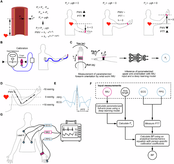
A Overview of how a non-zero hydrostatic pressure Ph contributes to transmural pressure Pt (i.e., by adding to the arterial pressure Pa, the quantity of interest). For example, for a BP sensor placed on an arm, lowering the arm increases Pt and PWV, and decreases the PTT measured compared to the case of a BP sensor at heart level. PWV and PTT relationships to arm levels below heart level, near heart level, and above heart level are illustrated. B Illustration of a commercial method for correcting for Ph, based on an initial calibration procedure where the reference sensors (at heart and fingers) are placed at the same vertical level, followed by continued hydrostatic pressure correction using a fluid-filled tube relative pressure sensor that connects heart level to the finger. C Overview of approach for Ph tracking. The approach uses wrist-based inertial sensors and a deep learning model to infer parameterized arm orientation, which is then used to calculate Ph to correct errors that result from height differences between BP sensors using an analytical biomechanics wave model. D Diagram illustrating changes in Ph along the arm relative to the heart. The arrows represent the pulse wave traveling down the arm, with arrow length corresponding to PWV magnitude. E PTT calculation from ECG and PPG waveforms. F Block diagram of the deep learning-assisted model and BP prediction pipeline. Arm pose is estimated from a wrist-based IMU and a deep learning model based on measurements from IMU and a parametrized arm-pose coordinate system; this arm pose information is used to calculate hydrostatic pressure (Ph). PTT is measured using ECG and PPG. A prediction of BP is made using an analytical pressure wave propagation model with inputs of PTT and Ph following person-specific calibration to calculate fitting coefficients. Pink denotes IMU for estimating Ph, and blue denotes devices for measuring PTT. G The devices used in this study were one lead ECG, finger PPG, and wrist-mounted IMU.
Here, we present a novel strategy to correct Ph errors in BP measurements derived from pulse transit time (PTT) using wearable inertial measurements unit (IMU) sensors and a deep-learning model (Supplementary Fig. 1) to estimate parameterized arm-pose coordinates, which are used as inputs to an analytical hemodynamics model to compensate for Ph (Table 1). Currently, without correction of Ph, fluctuations in Ph along the path of wave propagation affect PWV34,35, resulting in varying PTT measured across the limb36,37. In this work, we develop a method to correct BP measurements derived from PTT38,39, robust to varying positions of the sensor relative to heart level, and seek to demonstrate the validity of this method on data collected from sensors placed systematically at different heights. (A previous dataset available publicly40,41, as well as previous studies42,43,44,45, recorded PPG waveforms, in some cases with IMU data, but did not record the heights of sensors relative to heart level, or include systematic variations of sensor heights).
Results
Overview of approach of correction of BP measurement from PTT
Our overall approach, which we call IMU-Track, uses motion information collected from wearable sensors and a deep-learning model to correct Ph errors in BP measurements collected away from the heart level. The approach recognizes the biomechanics behind this error correction for PTT (Fig. 1A). PTT is inversely related to PWV, which increases in relation to transmural pressure Pt (i.e., an exponential relationship as described further in the Methods, Mathematical model section). The transmural pressure Pt, however, is composed of arterial pressure (i.e., the pressure one is interested in measuring) and external pressure effects, which include hydrostatic pressure. As an example of a Ph error, when the sensor is placed at a position lower than heart level, a positive hydrostatic pressure adds to the arterial pressure to increase Pt, which increases PWV and decreases the PTT measured (Fig. 1A). If Ph is known, it can be subtracted from the Pt calculated from PTT, to yield the true arterial pressure. The current state-of-the-art technology for measuring Pt (as used in the commercial Edwards ClearSight noninvasive continuous hemodynamics monitoring system) requires a calibration procedure which requires manual placement of a finger reference sensor at heart level, and continuous use of a liquid-filled tube placed from the finger to heart level and which is connected at one end to a pressure sensor that measures Pt (Fig. 1B).
Overview of IMU-track for hydrostatic pressure-corrected blood pressure estimation
By contrast, IMU-Track uses measurements from a wrist-based inertial measurement unit (IMU), which consists of an accelerometer, gyroscope, and magnetometer, and a deep learning model that estimates parameterized arm pose. This estimated pose and measured arm length are then used to calculate Ph for subsequent correction (Fig. 1C). We evaluate our approach using BP derived from PTT, which is affected by variations in PWV that arise from changes in Ph (Fig. 1D). In the demonstration of this study, PTT is calculated as the delay between the ECG R-wave peak and the onset time of the finger PPG waveform, defined as when the second derivative is maximized (Fig. 1E). While any fiducial point can be selected as the distal time reference, PTT calculated using PPG onset has been shown to correlate better to BP46. Finally, the calculated Ph and measured PTT serve as inputs into an analytical model of pulse wave propagation to predict BP. The block diagram detailing the full pipeline is shown in Fig. 1F, showing how arm pose of the upper arm and lower arm pitch is obtained from the IMU through a deep learning model; combined with arm length, the pitch angles are used to calculate Ph. In parallel, ECG and PPG are shown to produce PTT, which along with Ph, are used to estimate BP with an analytical biomechanics equation using person-specific calibration coefficients (see Methods). We demonstrate our approach using data collected from 20 human participants, with intake data summarized in Supplementary Table 3. The devices in this study consisted of one lead ECG, finger PPG, and wrist-mounted IMU (Fig. 1G).
Deep learning enables arm pose tracking
Towards developing a method for tracking relative elevation along the arm, we considered the arm as two rigid segments, the upper arm, and forearm, with lengths Lu and Lf, respectively (Fig. 2A). We defined the shoulder as the zero-Ph reference point instead of the heart to simplify calculations such that relative elevation is parameterized by the angles between the arm segments and the horizontal axis, θu and θf. This simplification is reasonable as the height difference between the heart and shoulder is small such that the Ph difference is minimal. If arm length is known, tracking relative elevation thus reduces to tracking these two angles, here defined as the arm pose. To minimize additional instrumentation, we sought to track pose using a single IMU, capable of directly measuring linear acceleration and orientation, at the wrist. The IMU was attached to the wrist with the positive x-axis pointing down the arm such that, after converting the measured forearm orientation to intrinsic ZYX Tait-Bryan angles (yaw, pitch, and roll), the pitch was equal to θf (Supplementary Fig. 2). For upper arm tracking, we modified Deep Inertial Poser47, which uses a two-layer, bidirectional48 long short-term memory49 (LSTM) model, to predict upper arm orientation given the current frame of forearm orientation and acceleration along with 19 past and 5 future frames (Fig. 2B). The deep inertial poser architecture was selected as the base model to be modified in part because of its established use-case for full-pose prediction using IMUs; also, two-layer, bidirectional LSTMs confer the benefit of bidirectional recurrent neural network architectures for improving context, and is commonly used for natural language processing50 and growing in popularity for motion analysis51. Orientation was represented as a unit quaternion that described rotation from the sensor-local frame to the global inertial frame. Acceleration was given in the global inertial frame with gravity canceled. The predicted upper arm orientation was then used to calculate θu. The model was pretrained using the Virginia Tech Natural Motion Dataset (VT-NMP) and fine-tuned on data collected using our IMUs. Fine-tuning was used to account for the subtle differences in the distribution between the datasets and to condition the model on the types of motion encountered during inference47. Model evaluation was performed using a leave-one-out cross-validation method whereby of the 20 participants, data from 19 participants were used for fine-tuning while data from the remaining participant was used for testing, and the procedure repeated until every participant was tested. The error histograms calculated on the test fold pooled across the 20 study participants (Fig. 2C) demonstrate that fine-tuning is critical, reducing the angular error between the measured reference and predicted θu from 44.2 ± 24.6° to 4.5 ± 11.2°. The time series of θu for a representative participant (Fig. 2D) shows that the prediction closely tracked the reference. While there are occasional deviations, they occur predominantly during sudden movement, and the predicted signal quickly reconverges to the ground truth. These results demonstrated that we can track arm pose using a single IMU sensor at the wrist. While the model was trained and evaluated using desktop graphic processing units, the trained model could be deployed in a mobile device that interfaces directly with the IMU for on-device inference. To estimate the inference speed for this scenario, the model was first converted into a format suitable for mobile devices using TensorFlow Lite52. The model was then deployed in a commercial smartphone, and the inference time was benchmarked (Fig. 2E). For the full-precision model, the average inference time was 134.2 ± 3.9 ms. As this is shorter than a cardiac cycle (for reference, 250 ms for a very fast heart rate of 240 beats per minute), the model is sufficiently fast for Ph correction in real-time BP tracking applications, and meets the definition of being a ‘continuous’ BP output frequency per ISO 81060-3:2020. If the model were to be deployed in devices with lower computational power, such as smartwatches or fitness trackers that already contain the required inertial sensors, the model weights could be quantized to lower precision to shrink the model size and decrease the required compute with minimal degradation in accuracy. Specifically, after 8-bit quantization (i.e., reducing the model weights from 32-bit to 8-bit precision), the inference time was reduced to 35.5 ± 1.1 ms while incurring only a 0.5° loss in average accuracy.
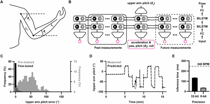
A Schematic diagram showing a parameterized model for arm pose. Positive θ indicates moving the corresponding limb upward. B Deep learning architecture diagram for tracking upper arm orientation (θu). The inputs at each timestep are forearm acceleration and orientation (i.e., yaw, pitch θf, and roll) represented as a unit quaternion. These inputs are fed through a fully connected (FC) layer followed by two bidirectional LSTM (BiLSTM) layers. The latent feature vector for the current timestep is then passed through a final FC layer to predict the upper arm orientation quaternion, normalized to the unit norm. The orientation quaternion is finally used to calculate θu. (C) Histogram of absolute errors for θu prediction for the model pretrained on the Virginia Tech Natural Motion Dataset alone (“pretrained”) and after fine-tuning on in-house training data (“fine-tuned”). D Time series of predicted and measured θu for a representative participant from a test fold. E Mean inference time for the arm-tracking model with 32- and 8-bit weight precision when run on a commercial smartphone. The dashed line indicates the cardiac cycle duration for a heart rate of 240 beats per minute (BPM). Data were represented as mean ± standard error of the mean (n = 50 for 32-bit and 8-bit).
Modeling the effect of arm pose on PTT
Starting from the Moens–Korteweg and Hughes53 equations, we derived an ordinary differential equation to model pulse wave propagation as a function of arm pose and BP. By assuming arm pose is constant for a cardiac cycle, the equation was integrated, yielding a model for PTT (T) as a function of BP (P) and arm pose (θu and θf):
where ρ is blood density, g is the acceleration due to gravity, and k1 and k2 are person-specific fitting coefficients (see the “Mathematical model” section in Methods for the full derivation). Inspection of these equations shows that PTT is a sum of two uncorrected partial transit times, describing travel along the upper (Tu) and lower arm (Tf), weighted by correction factors (αu and αf) that compensate for the effects of Ph. Simulations (Fig. 3A and Supplementary Fig. 3) revealed that, for a fixed arm pose, PTT decreases monotonically with increasing BP; however, changes in arm pose were found to cause substantial variation in predicted PTT for a given pressure, with the effect minimized for large pressures.
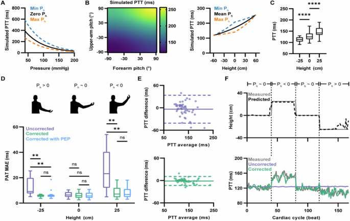
A Relationship between pressure and simulated PTT. A solid black line indicates simulated PTT without Ph effects. Dashed blue and orange lines indicate simulated PTT with Ph minimized and maximized via straight up and down poses, respectively. B Left: heatmap of simulated PTTs for constant BP over all possible arm pose configurations. Positive pitch indicates moving the corresponding limb upward. Right: projection of heatmap simulation with arm pose converted to hand height. A solid line indicates simulated PTT with average Ph effects (i.e., where θu = θf). Dashed blue and orange lines indicate simulated PTT with Ph minimized and maximized, respectively. C Across n = 20 participants, box plots of measured PTT were taken at different hand heights. Each measurement was the participant’s time-averaged PTT for the indicated height (for h = −25, 0, and 25 cm, n = 20, 20, and 19, respectively). Significance determined by mixed-effects model followed by Dunnett post hoc test. For h = −25 vs h = 0 cm, ****P < 0.0001; for h = 0 vs h = 25 cm, ****P < 0.0001. Individual trajectories in Supplementary Fig. 5. D Across n = 20 participants, box plots of h-stratified MAE for best-fit PTT predictions generated using the uncorrected and corrected models, with or without PEP, compared to the measured reference. Each measurement was the participant’s time-averaged MAE for the indicated h. The diagrams above show an illustrative example of the arm pose corresponding to each group (for h = -25, 0, and 25 cm, n = 16, 20, and 15, respectively). Significance determined by mixed-effects model followed by Šídák post hoc test; **P < 0.01; ns, not significant). Individual trajectories in Supplementary Fig. 7. E Repeated measures Bland-Altman plots for the best-fit PTT predictions from the uncorrected (top) and corrected model (bottom) compared to the measured reference across time-averaged participant and height pairs (n = 51; 2 to 3 measurements from each of the 20 participants). The X-axis shows the average of prediction and reference, and the y-axis shows the difference between prediction and reference. The solid line indicates the mean difference, and the dashed line indicates 95% LoA. The enlarged version shows the values of h in Supplementary Fig. 8. F A representative participant’s time series of measured and predicted hand height (top); corresponding time series of PTT predicted using the uncorrected and corrected models compared to the measured reference (bottom). Time series of representative participants PTT prediction error in Supplementary Fig. 10. For (C, D), the box represents the interquartile range, with the horizontal line at the median value. The vertical lines extend to the maximum and minimum data points within 1.5 × IQR.
To further investigate the impact of arm pose, we simulated PTT over a grid of arm pose specifications with constant pressure (Fig. 3B, left). As expected, the model predicted an increase in PTT with increasing arm pitch (indicating moving the limb upward), as this movement causes a decrease in Ph and a subsequent decrease in PWV. Conversely, the simulations showed a decrease in arm pitch resulted in a decrease in PTT. As controlling both θu and θf in an experimental setting is challenging, we also explored the effects of Ph on PTT due to the relative height of the distal measurement site (h) alone (Fig. 3B, right and Supplementary Fig. 4). Based on these simulations, PTT tends to increase with increasing h; however, the model predicts an asymmetric, nonlinear relationship where an increase in h causes a larger increase in PTT than the equivalent decrease in h. The simulations also demonstrated the importance of using arm pose, rather than h alone, for Ph compensation. In particular, as the arm pose has two degrees of freedom (θu and θf), PTT can vary independently of central pressure even when h is fixed. As a result, the simulations showed a distribution of PTTs for a given h and fixed BP that is widest when h = 0 cm and narrow at the extremes.
Experimental evaluation of an analytical model for wave propagation
To validate the mathematical model, we recorded PTT in 20 participants as they moved their arms through a sequence of movements to vary h between −25, 0, and 25 cm. Matching the simulations, a decrease in h resulted in a significant decrease in PTT (P < 0.0001) while an increase in h resulted in a significant increase in PTT (P < 0.0001) (Fig. 3C and Supplementary Fig. 5). Next, we sought to evaluate how well the model “corrected” for Ph effects fit the measured PTTs, compared to an “uncorrected” model that fixed αu and αf to 1 and thus did not account for hydrostatic effects. Along with the “uncorrected” and “corrected” models, we also considered a third model that, in addition to correcting for Ph, accounted for the pre-ejection period (PEP), the time between the depolarization of the left ventricle (indicated by the R-wave peak) and ventricular ejection54. Due to the PEP, the ECG-to-PPG delay used to estimate PTT overestimates the true value; thus, we explored explicitly accounting for this deviation. As intra-individual variability for PEP is low55, we modeled it as a person-specific constant bias that is added to the upper arm and forearm partial transit times (Tpep):
To calculate the person-specific fitting coefficients (k1 and k2 or k1, k2, and Tpep), personalized calibration was performed. For each participant, the measured data were divided into two non-overlapping windows, one for calibration and the other for testing. The calibration data were then used to find the person-specific coefficients by minimizing the mean squared error between the measured and predicted PTT with mean arterial pressure as P. After calibration, best-fit PTT predictions were generated for the calibration data using the personalized models; the best-fit PTTs were then compared to the measured PTTs to assess model performance.
We first assessed the absolute fit of the models to the calibration data across all participants, with results summarized in Supplementary Table 4. Compared to the “uncorrected” model, both pose-corrected models had significantly reduced mean absolute error (MAE) between measured and best-fit PTT (Supplementary Fig. 6), with an average improvement of 4.2 ± 0.7 ms (P < 0.0001) and 4.2 ± 0.7 ms (P < 0.0001) for the “corrected” and “corrected with PEP” models respectively. Moreover, reduced MAE was observed for each h (Fig. 3D and Supplementary Fig. 7). For the “corrected” model, there was an average improvement of 7.6 ± 1.7, 0.8 ± 0.3, and 17.2 ± 3.4 ms for h = -25, 0, and 25 cm, respectively (P = 0.0035, P = 0.1978, and P = 0.0014). For the “corrected with PEP” model, the average improvement was 7.6 ± 1.7, 0.9 ± 0.3, and 17.5 ± 3.3 ms for h = -25, 0, and 25 cm, respectively (P = 0.0038, P = 0.1425, and P = 0.0011). Significant reduction in MAE for h = 25 cm and h = -25 cm was expected, as the uncorrected baseline is unable to account for the Ph-induced change in PTT that follows a change in hand height.
Comparing the two pose-corrected models, the inclusion of the additional PEP term reduced the MAE, but the effects were minimal (ranging from 1–2%) and not significant at the heights assessed (P > 0.99999, P = .3980, P = 0.8164 for h = -25, 0, and 25 cm, respectively). Based on the change in the corrected Akaike’s information criteria56, the additional PEP variable did not significantly improve the fit to the measured data (P = 0.5697). Therefore, because it was more parsimonious, the pose-corrected model without the explicitly modeled PEP was used for subsequent analysis. Nevertheless, these results demonstrate that our model can incorporate the PEP. Overall, the ECG-to-PPG delay can be used as an estimate for the underlying PTT with minimal performance loss. Alternatively, a second PPG worn on the upper arm could be used as the proximal timing reference in place of ECG, enabling direct measurement of PTT without overestimation due to PEP.
We next assessed the agreement between the measured PTT and the “uncorrected” and “corrected” model predictions. Bland-Altman plots comparing the measured and best-fit estimates for PTT (Fig. 3E and Supplementary Fig. 8) indicated that pose correction improved both bias and precision, resulting in a tightening of the 95% limits of agreement (LoA). In addition to improving absolute fit and agreement, the pose correction significantly improved the correlation of the best-fit PTT predictions to the measured PTT, with the repeated measures correlation increasing from −0.09 to 0.96 (P < 0.0001) (Supplementary Fig. 9).
Finally, we looked at the performance of the “uncorrected” and “corrected” models over time for a representative participant (Fig. 3F). For the calibration data, the height-tracking time series (Fig. 3F, top) demonstrated that the predicted pose from the deep learning model could track hand elevation ground truth. The beat-to-beat, best-fit PTT predictions (Fig. 3F, bottom and Supplementary Fig. 10) indicated that the uncorrected baseline failed to track the measured PTT, with an increased error when h was non-zero. Specifically, in regions where the arm was raised, and Ph was negative, the uncorrected model underestimated the measured PTT. Conversely, when the arm was lowered, resulting in positive Ph, the uncorrected model overestimated the measured PTT. By comparison, the pose-corrected model closely tracked the measured PTT for the entire calibration interval (Fig. 3F, bottom and Supplementary Fig. 11), indicating that the corrected-pose equations better fit the measured data.
Blood pressure predictions using a pose-corrected model
We next sought to evaluate the model when used for BP prediction. By rearranging Eq. 1 to solve for BP, we arrive at the following pose-corrected BP model:
We applied two separate BP models for diastolic (DBP) and systolic pressure (SBP). For personalized calibration, we minimized the mean squared error between the calibration subset of the measured BP and the predictions from the pose-corrected BP model to obtain person-specific values for the coefficients k1 and k2. The models were then evaluated on the held-out test data not seen during calibration. To assess the importance of pose correction, we compared the accuracy of BP estimates generated with the Ph-compensated “corrected” model with that of an “uncorrected” model (i.e., with αu and αf set to 1).
Across all participants, the corrected model significantly reduced overall MAE to 6.8 ± 0.4 (P < 0.0001) and 5.9 ± 0.5 mmHg (P < 0.0001) for DBP and SBP, respectively (Supplementary Fig. 11 and Supplementary Fig. 12). Significant improvement in MAE was consistent across h for DBP predictions (Fig. 4A, middle and Supplementary Fig. 13), with MAE reduced to 6.8 ± 0.5, 6.5 ± 0.5, and 7.8 ± 0.8 mmHg for h = -25, 0, and 25 cm, respectively (P < 0.0001, P = 0.0356, and P = 0.0096). Significantly reduced MAE was also found at each h for SBP prediction (Fig. 4A, bottom and Supplementary Fig. 14), with MAE reduced to 5.9 ± 0.7, 5.8 ± 0.6, and 5.9 ± 0.5 mmHg for h = -25, 0, and 25 cm, respectively (P < 0.0001, P = 0.0284, and P = 0.0051). Critically, there was no significant difference in MAE across the different values of h when using the corrected model for DBP (P = 0.2217) or SBP (P = 0.9906) prediction. These results are summarized in Supplementary Table 5.
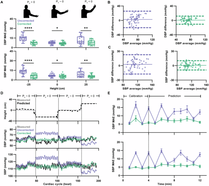
A Box plots of h-stratified MAE for DBP (middle) and SBP (bottom) predictions generated using the uncorrected and corrected model compared to the measured reference across 20 subjects with n = 19, 20, and 19 measurements for heights of h = −25, 0, and 25 cm, respectively. Each measurement was the participant’s time-averaged MAE for the indicated h. The box represents the interquartile range, with the horizontal line at the median value. The vertical lines extend to the maximum and minimum data points within 1.5 × IQR. The diagrams (top) show an illustrative example of an arm pose corresponding to each group. Significance determined by mixed-effects model followed by Šídák post hoc test. (DBP: for h = -25 cm, ****P < 0.0001; for h = 0 cm, *P = 0.0356; for h = 25 cm, **P = 0.0096. SBP: for h = -25 cm, ****P < 0.0001; for h = 0 cm, *P = 0.0284; for h = 25 cm, **P = 0.0051). Individual trajectories in Supplementary Figs. 13 and 14. B, C Repeated measures Bland-Altman plots using the uncorrected and corrected model compared to the measured reference for DBP (D) and SBP (E) prediction across time-averaged participant and height pairs (n = 58; 2 to 3 measurements from each of the 20 participants). The X-axis shows the average of prediction and reference, and the y-axis shows the difference between prediction and reference. The solid line indicates the mean difference, and the dashed line indicates 95% LoA. Enlarged versions showing the values of h in Supplementary Figs. 15,16. D A representative participant’s time series of measured and predicted hand height (top); corresponding time series of DBP and SBP predicted using the uncorrected and corrected models compared to the measured reference (bottom). Time series of representative participant’s BP prediction error in Supplementary Fig. 17. E Participant-aggregated MAE over time for DBP (top) and SBP (bottom) predictions using the uncorrected and corrected model. The first 4 min of data were used for calibrating the models, while the following 8 min were used for prediction. Data were represented as mean ± standard error of the mean (n = 13 to 20 for each point, across the 20 subjects).
In addition to reduced MAE, the corrected model improved agreement. The Bland-Altman plots for the measured reference pressure compared to the model predictions (Fig. 4B, C and Supplementary Figs. 15, 16) revealed that the inclusion of the pose correction improved both the bias and precision of the pressure estimates, resulting in greater agreement as indicated by the tightening of the 95% LoA. The mean error (ME) for DBP and SBP prediction was reduced to 0.7 ± 5.7 mmHg and 0.7 ± 4.9 mmHg, respectively, which meets the accuracy criteria for the Association for the Advancement of Medical Instrumentation/European Society of Hypertension/International Standards Organization (AAMI/ESH/ISO) validation standard57.
Finally, we assessed the accuracy of the BP predictions over time. For a representative participant, the relative height time series (Fig. 4D, top) for the test set indicated that the deep learning model tracked h. From the beat-to-beat pressure predictions (Fig. 4D, bottom and Supplementary Fig. 17), it was found that the predictions generated from the uncorrected and corrected models were comparable when h = 0 cm, as θu and θf were both near 0° and thus minimized hydrostatic effects. However, predictions for both DBP and SBP made using the uncorrected model tended to underestimate the measured reference when h = 25 cm and overestimate when h = −25 cm. With pose correction, the pressure predictions more closely tracked the reference for both conditions. Across all participants, we examined the MAE for both DBP and SBP predictions over time (Fig. 4E). We found that the predictions generated with the corrected model had lower errors for the entire measurement period compared to the predictions generated with the uncorrected model. Moreover, we found that there was not a significant trend in the accuracy of the corrected model’s predictions with time (P = 0.6330 and P = 0.7536 for DBP and SBP, respectively), indicating that the model’s performance is stable over time assessed. To further understand the performance of the model, we also calculated the Clarke error grid for the SBP predictions58 from all patients (Supplementary Fig. 18). It was found that approximately 94.8% of the SBP predictions were classified as no risk, with the remaining 5.2% classified as low risk, indicating that the discrepancy from the reference SBP would be unlikely to result in adverse outcomes. We also performed sensitivity analysis to assess the robustness of the deep-learning model to variations in user arm length (Supplementary Figs. 19, 20). The analysis showed high accuracy for predicting upper arm pitch for both the pretrained model and the fine-tuned models, consistently across arm lengths.
Taken together, we thus conclude that the corrected model is able to compensate for Ph effects, enabling accurate BP prediction under conditions of varying h induced by changes in arm position.
Discussion
We present IMU-Track, a method for Ph correction in BP measurements taken away from heart level by tracking motion of the sensor. This method is validated with data provided from a sample of 20 subjects, with Ph correction performed for heights 25 cm above and below the heart. The use of motion data, such as acceleration, to infer position is not trivial; for example, previous attempts to double integrate accelerometer data incurred errors (e.g., accumulation of errors took place even in the absence of motion of the accelerometer from both sensor noise and quantization errors in the integration)59. In IMU-Track, as demonstrated by sensors placed on the wrist (which can incur significant changes in position relative to heart level), position is tracked in a parameterized arm-pose coordinate system where a wrist-worn IMU measures θf, and a deep learning model uses forearm acceleration and orientation from the IMU to infer θu. We described an analytical model for PTT as a function of BP and arm pose, which—given measures of PTT and arm pose— reported corrected estimates of BP (i.e., bias and precision meeting clinical accuracy criteria, and with no significant difference in accuracy across arm position that varied hand elevations). While we demonstrated the method of error correction for BP measurements based on PTT, the method for determining Ph is independent of how the BP measurements are made, and hence could be applicable to other modes of cuffless BP measurements (e.g., pulse wave analysis, EKG, tonometry, or ultrasound) where the sensors are placed away from the heart level. Different criteria can be used for evaluating PPG-based algorithms toward BP assessment60; this study reports MAE, ME, R, and Bland-Altman compared to the reference.
IMU-Track can potentially improve the accuracy of future cuffless devices in and outside the hospital. In the hospital, current devices for BP measurement in critically ill patients include cuff-based devices that obtain frequent measurements but may disturb the user during the nighttime period21, and also do not correct for Ph fluctuations caused by changes in the location of the patient’s arm relative to the heart; in the future, IMU-Track could correct BP measurements from ECG and finger PPG signals, which are already routinely monitored in critically ill patients61,62,63,64. Notably, the systems employing hydrostatic pressure correction at present do so obtrusively (Supplementary Fig. 1). In an office or home setting, IMU-Track can potentially correct BP measurements from wireless physiological monitors65 placed away from heart level, or those taken on smartwatches containing ECG electrodes66,67 and PPG sensors. Our method uses IMU sensors which have been widely used to measure joint angles (e.g., to within 5o)68 and deduce complex motion, via form factors that are small, portable, and low-power68,69. The overall small form factor required for IMU-Track is appropriate for wearing in settings from hospitals to homes.
Future work could explore methods for even simpler calibration procedures23, as well as larger sample sizes to meet clinical and regulatory standards57 and ranges of participant-specific parameters (building on the range of age, body mass index, and BP status in the current study, Supplementary Table 3). Studies can also assess the effectiveness of IMU-Track for different sensor placement and alignment, motions across diverse daily activities, and long-term accuracy and stability.
Methods
Study design
The purpose of the study was to develop a method for compensating for the effects of Ph using wearable inertial sensors at the wrist to enable accurate BP prediction across different arm positions without requiring recalibration. To validate the method, a human study was performed under protocols approved by the Institutional Review Boards at Columbia University Medical Center (IRB no. AAAR5932) and with written, informed consent from all participants. 20 adult participants were recruited from the student and staff population at Columbia University Medical Center. The exclusion criteria were a history of (1) Raynaud’s phenomenon or vascular disease involving the upper extremities, (2) history of cardiovascular disease, (3) uncontrolled hypertension, and (4) pregnancy. Sex, age, BMI, and other parameters in our sample population reflected the natural distribution among students and staff at Columbia University. A summary of intake data for the recruited participants is found in Supplementary Table 3.
The study fit participants with noninvasive sensors (specified in the Data Collection section) and guided them through various arm movements, with the resulting data recorded for analysis. We first trained a deep-learning model for arm position tracking. The deep learning model was pretrained using the VT-NMP dataset70. Fine-tuning and testing of the model was then performed using the inertial sensor data from the human participants. Next, an analytical equation of PTT under the effects of varying Ph was derived and computationally modeled to understand how arm position affects PTT. A subset of the data collected from each participant was used to experimentally validate the derived PTT model. Finally, we evaluated the performance of this analytically derived model for BP prediction across varied arm positions. A subset of data was used for personalized calibration of the BP prediction model for each participant. The calibrated models were then evaluated on the remaining held-out data for each participant. Investigators were not blinded during the study. The sample size (n = 20) was chosen according to a cuffless BP validation standard (IEEE 1708a-2019) that specifies 20 participants for the initial pilot phase71.
Data collection
Each of the 20 participants was fit with various noninvasive sensors and devices, including continuous noninvasive BP measurement device (BIOPAC NIBP), ECG electrodes (3M Red Dot 2237), two PPG sensors (BIOPAC TSD200), and two IMU devices that contained a combination accelerometer/gyroscope (STMicroelectronics LSM6DSM), magnetometer (STMicroelectronics LIS2MDL), and motion coprocessor (EM Microelectronics EM7180). Additionally, arm length (from humeral head to radial styloid with the arm abducted to 90o with the elbow extended with the thumb facing up) and hand length were recorded for each participant. The BIOPAC NIBP was operated in a contralateral setup where the upper arm cuff was attached to the participant’s non-dominant arm, and the two finger cuffs were placed around the index and middle fingers of the dominant hand. Prior to initial calibration, both arms were placed on armrests located at heart level. The upper arm cuff was then used to acquire an initial BP measurement, while the finger cuffs acquired subsequent beat-to-beat BP measurements. The dominant arm with the finger cuffs was maintained at heart level for the duration of the experiment. The ECG electrodes were placed in Lead II configuration, and the signal was fed into an amplifier (BIOPAC ECG100C). The PPG sensors were attached to the ring finger of each hand and fed into separate amplifiers (BIOPAC PPG100C). The output from these sensors was recorded using a digital acquisition system (BIOPAC MP160) at 2000 Hz. The two IMUs were affixed to the upper arm and the wrist of the non-dominant arm. The sensors were aligned such that the sensor-frame positive x-axis pointed down the arm. The sensors were controlled using a microcontroller (PJRC Teensy 3.6). Data were collected at 100 Hz and logged to a microSD card. Synchronization of data acquisition was accomplished using a digital output signal from the MP160.
After an initial 5-min period of rest to acquire baseline readings (with both arms at heart level), the participants were asked to raise or lower their non-dominant arm to the designated armrest, located 25 cm above or below heart level, to cause a Ph perturbation. The participant was instructed to rest at the new position for 1 minute. After the minute had elapsed, the participants were instructed to move their non-dominant arm to another position with a 1-min rest. This procedure was repeated until the participant had completed a sequence of 11 movements to one of three armrests (25 cm below heart level, heart level, or 25 cm above heart level). Participants were randomly assigned to one of two movement sequences, either [0, 25, 0, −25, 0, −25, 0, 25, −25, 25, 0, −25] or [0, −25, 0, 25, 0, 25, 0, −25, 25, −25, 0, 25], with the first height indicating the initial rest period. After the sequence of arm movements was completed, the data was saved for downstream analysis.
IMU data preprocessing
For in-house IMU data, acceleration and orientation data were first re-oriented. The data was then filtered using a smoothing filter and decimated for downstream analysis. For the VT-NMP dataset, re-orientation and decimation of the data were also performed to parallel the preprocessing of the in-house IMU data. Acceleration was represented with gravity removed. Orientation was represented as a unit quaternion. Following this, the IMU data was passed onto the deep learning model for sequential pose prediction. Data were not discarded during instances of motion.
Deep learning model architecture and training
The deep learning model was implemented in Python with the PyTorch library and was trained on an Nvidia RTX 2080 Super GPU. Pose prediction was performed using a modified implementation of the Deep Inertial Poser47 architecture. The model had four layers: (1) a time-distributed fully connected layer, (2) a bidirectional LSTM layer, (3) a second bidirectional LSTM layer, and (4) a time-distributed fully connected layer upper arm orientation prediction. The predicted quaternion was then normalized to the unit norm. Finally, the quaternion was used to calculate θu. The input to the model was a sequence of forearm orientation and acceleration. The output was the corresponding sequence of θu. During pre-training and fine-tuning, the model was used in the many-to-many scheme, with the loss minimized over the full prediction sequence. During inference, a single θu was predicted for each input sequence, as shown in Fig. 2B.
For pretraining with the VT-NMP dataset, we used the same training and validation split proposed by Geissinger and Asbeck72. For each participant, the full motion sequence was used to construct batches of partially overlapping sub-sequences using a sliding window. The model weights were randomly initialized and trained to minimize the MAE loss by stochastic gradient descent. To prevent overfitting, validation loss was monitored to implement early stopping. Model hyperparameters were optimized based on performance on the validation split.
For fine-tuning and model evaluation, we used a leave-one-out cross-validation method73,74. The IMU data was split into 20 folds, with each fold comprising the data from a single participant. For each iteration of cross-validation, data from 19 folds were used for fine-tuning, while data from the remaining fold was used for testing. During fine-tuning, the first 90% of data from each participant was used for training, while the remaining 10% was used for validation. Data were preprocessed into partially overlapping sub-sequences, as described previously. The model weights were initialized using the weights from the model pretrained on the VT-NMP dataset. The model was trained by stochastic gradient descent to prevent overfitting, validation loss was monitored to implement early stopping. During testing, sub-sequences were created from the held-out fold using a sliding window. The input sequences were passed through the model to generate sequences of predicted θu. A single pose corresponding to the current timestep was extracted from the prediction sequence. Pitch time series were then reconstructed by concatenating all predictions for that participant. This procedure was repeated until every fold was used for testing.
On-device inference
The full-precision PyTorch model was first exported into the Open Neural Network Exchange (ONNX) format. The resulting ONNX model was then converted to TensorFlow75. Finally, the TensorFlow model was converted to TensorFlow Lite52 for on-device inference. For the full-precision model, the network weights were maintained at 32-bits during the TensorFlow Lite conversion. However, for the quantized model, the weights were reduced to 8-bits. To measure inference time on-device, the Android benchmark application was used. The benchmark application was used to find the average model inference time over 50 runs. The benchmark was performed on a Google Pixel 4a smartphone using one processing thread and one warmup run. Data were presented as mean ± standard deviation.
Mathematical model
Arm PTT is a measure of the time it takes for the BP pulse wave to travel from the heart to a distal measurement site. It is thus a function of the velocity of this wave (PWV) and arm length (L). By the Moens–Korteweg equation76, PWV (c) can be related to the elastic modulus (E), vessel thickness (w), vessel diameter (d), and blood density (ρ) as follows:
By the empirically derived Hughes equation53, the elastic modulus is exponentially related to the transmural pressure (Pt):
Here, E0 is the elasticity when Pt is zero and α is a constant. Substituting the Hughes equation into the Moens–Korteweg yields an expression for c as a function of Pt:
If the ratio (sqrt{{E}_{0}w/rho d}) is assumed constant, this equation can be simplified by defining new constants, k1 = (sqrt{{E}_{0}w/rho d}) and k2 = (frac{1}{2}alpha), as follows:
Thus, as the wave travels to the distal site, PWV varies depending on the transmural pressure at each point along the arm. To account for these variations, first substitute in the definition for Pt:
where Pa is the intra-arterial pressure and Pext is the external pressure. Next, we assume pulse pressure amplification is negligible along the arm such that Pa = P. Further, we assume Pext is dominated by Ph. Substituting for Pa and Pext yields a model for PWV as a function of BP and Ph:
We next let Ph = -ρgh where ρ is blood density, g is gravitational acceleration, and h is the height of the distal measurement site relative to the reference point (e.g., the heart), with the upward direction treated as positive (i.e., h > 0 indicates a position above the heart). Substituting for Ph:
To find PTT, first substitute in the differential definition of c:
where x is the position of the wave along the arm and t is time. Rearrange and then integrate to yield PTT,
Note that h is a function of the distance the wave has traveled. Thus, h must be redefined in terms of x. To do so, parameterize the arm as two rigid bodies (upper arm and forearm) of lengths Lu and Lf. Next, let the point of reference for relative altitude be the shoulder (i.e., x = (0)) such that the relative altitude for any point along the arm can be defined as follows:
where θu is the upper arm pitch and θf is the forearm pitch, with a positive pitch indicating moving the limb upward. Next, split the integral into upper arm and forearm components, as follows:
If θu and θf are assumed constant for a cardiac cycle, Eq. 14 can be directly integrated, yielding Eq. 1, the model for PTT with Ph effects compensated using arm pose. Rearranging this equation to solve for P yields Eq. 3.
PTT simulation
PTT was simulated with Eq. 1 using MATLAB. For all simulations, the parameters were k1 = 80 cm·s−1, k2 = 0.0165 mmHg−1, P = 90 mmHg, and L = 60 cm with Lu = Lf = ½ L, unless otherwise noted. For simulations showing the PTT-BP relationship, BP was varied from 50 to 200 mmHg in increments of 5 mmHg. For simulations showing the relationship between PTT and arm pose, θu and θf were varied from −90 to 90° in 5° increments.
PTT, pose, and BP data preprocessing
Raw PPG recordings were filtered. Additionally, 5 seconds of data between h transitions were dropped, to remove data from known periods of motion. Onset times were identified as the peaks in the twice-differentiated signal that occurred prior to a PPG peak. ECG data were used without additional cleaning. The R-wave peaks were identified as the proximal pulse reference. PTT was calculated as the time difference between a PPG onset and the preceding R-wave peak.
The deep learning model was used to generate arm pose estimates for each participant using the preprocessed IMU data. The arm pose predictions were upsampled to 2000 Hz. For each PTT, the arm pose corresponding to the R-wave peak and PPG onset were averaged and used to approximate the arm pose for that cardiac cycle.
Raw BP signals were filtered using a second-order low-pass Butterworth filter with a cutoff frequency of 30 Hz. DBP and SBP were identified as the minimum and maximum of each beat, respectively. Mean arterial pressure was calculated as (frac{2}{3})·DBP + (frac{1}{3})·SBP, a commonly used approximation77. BP was matched to the PTT calculated from the simultaneously acquired PPG beat.
Calibration for best-fit PTT prediction
For each participant, data corresponding to the initial rest period and the first three movements (i.e., the first ~8 min of data) were used for a one-time initial calibration, with the remaining eight movement stages held out for testing. The first four minutes of data from the rest stage was discarded, as the initial minutes were excessively noisy for many participants. For the model defined in Eq. 1 without PEP, the person-specific coefficients, k1 and k2, were found by minimizing the mean squared error between measured and predicted PTT with mean arterial pressure as (P). For the PEP-included model defined in Eq. 2, PEP was treated as a person-specific constant bias that was added to the upper arm and forearm partial transit times. The person-specific coefficients, k1, k2, and PEP were found by minimizing the mean squared error between measured and predicted PTT with mean arterial pressure as (P), as described previously. During calibration of the “uncorrected” baseline model, θu and θf were constrained to 0° (i.e., αu and αf set to 1). For the “corrected” model, θu and θf were the respective predicted and measured arm pitch from IMU-Track.
Best-fit PTT Prediction
After calibration, best-fit PTT predictions were generated with Eq. 1 or Eq. 2 using the same data used for calibration. During PTT prediction, the uncorrected baseline model constrained pitch to 0°.
Calibration for BP prediction
For the one-time initial calibration, the person-specific calibration coefficients were found by minimizing the mean squared error of reference (measured) and predicted BP on the data previously used for PTT model calibration mentioned above. For DBP prediction, the model was initially calibrated using DBP as P. Similarly, the model was initially calibrated with SBP as P for SBP prediction. In the same way as above, during calibration of the “uncorrected” baseline model, θu and θf were constrained to 0° (i.e., αu and αf set to 1). For the “corrected” model, θu and θf were the respective predicted and measured arm pitch from IMU-Track.
BP prediction
After calibration, BP predictions were generated with Eq. 3 on the testing data for each participant. During prediction with the uncorrected model, both θu and θf were constrained to 0°.
Statistical analysis
For statistical analysis between two groups with matched samples, a paired two-tailed Student’s t-test was used. For comparison between multiple groups of matched samples with one variable, a mixed-effects model with Dunnet post hoc test for multiple comparisons was used. For analyzing multiple groups of matched samples with two variables, a mixed-effects model with Šídák post hoc test for multiple comparisons was used. For analysis of repeated measures correlation coefficients, the Williams’ test for comparing two dependent correlations sharing one variable was used. Significance was considered for P < 0.05. All data were expressed as the mean ± standard error of the mean unless otherwise indicated. Statistical tests were calculated in GraphPad Prism 9.0.
Responses