A neural operator for forecasting carbon monoxide evolution in cities

Introduction

Indian cities, epicentres of economic prosperity and cultural vibrancy, are poised to accommodate over 675 million residents by 2035¹. The rapid urbanisation, alongside rampant industrialisation and a burgeoning population, has triggered a notable surge in the concentration of airborne pollutants such as Carbon Monoxide (CO), a criteria pollutant extensively studied historically to gauge urban air quality^2,3,4,5,6. While CO is recognised as an excellent tracer for atmospheric dynamics⁷, it plays a pivotal role in tropospheric ozone chemistry⁸ and exerts a profound impact on climate dynamics⁹. Furthermore, CO impacts neurodevelopment in children^10,11, and is associated with cardiovascular diseases^12,13.

Incorporating air quality management into policymaking for the development of sustainable urban centres is crucial^14,15,16. Traditionally, data from ground-based analysers is utilised to prioritise air quality management scenarios¹⁵. However, a low-density monitor network fails to capture spatial variations; for instance, India has 544 ground-based continuous monitoring stations measuring CO¹⁷, suggesting that the current state of air quality monitoring in Indian cities is inadequate^18,19. This challenge can be addressed by supplementing ground-based observations with air quality models to enhance the spatial coverage. Several studies have compared the performance of air quality models such as Model for Ozone and Related Tracers (MOZART)^20,21,22,23 and Weather Research and Forecasting-Chem (WRF-Chem)^24,25,26,27 with ground-based observations and satellite retrievals for CO. Despite their widespread usage, the performance of these models ranges from poor to moderate, often resulting in underestimation of pollutant concentrations. Additionally, computations become increasingly expensive due to the involvement of the chemistry module and the enhanced spatial and temporal resolutions required²⁸. These computations are performed for every instance with new initial boundary conditions, increasing the time required to make new simulations²⁹.

Data-driven machine learning (ML) models are gaining attraction as substitutes for these conventional models, given the availability of large amounts of data for training. ML models offer the distinct advantage of rapidly generating inferences on new instances with significantly lower computational demands. Various ML algorithms such as Linear Regression, Artificial Neural Networks, K-nearest neighbour, Support Vector Regression, Long short-term memory, and Convolutional Neural Networks (CNNs) were employed by several authors in the past to simulate CO^{30,31,32,33,34,35,36,37,38,39,40}. Several approaches were explored towards modelling pollutant concentrations using ML at much finer resolutions for urban scales^{41,42,43,44,45} with similar work applied at coarser resolutions for regional and country scales^46,47,48. Such models can facilitate the generation of information regarding pollutant concentrations in the absence of monitoring stations.

However, these ML models learn the function map between the finite-dimensional input and output spaces and need to be retrained for each new case i.e. a separate model for every new city. CNN-based models further incorporate local convolution to account for the nearby grid’s contribution, whereas modelling air pollution can be better represented using global convolution as it is a continuous function, being a solution of the advection-diffusion equation. These issues can be mitigated by adopting the approach from conventional models—learning the infinite-dimensional operator between input and output function spaces using partial differential equations with global convolution filters. Such a data-driven model would also address the constraints related to mesh dependency and resolution invariance⁴⁹. CO, like any other air pollutant, has its concentration influenced by factors such as emissions (primarily from combustion processes), meteorological conditions, and terrain characteristics. However, CO is relatively inert, with dilution predominating chemistry. This characteristic simplifies CO modelling, making it a preferable choice for investigating the potential of operator learning in pollution modelling in urban cities. Some approaches in this direction include the work on Fourier Neural Operator (FNO)⁵⁰, which can learn the map between initial boundary conditions to the time evolution of further steps. However, these models rely on stationary signals and do not perform well for modelling pollutants such as CO, which are inherently non-stationary.

To address the challenges of (a) expensive computations, (b) slow inference speeds, (c) inability of previous ML models to learn the underlying dynamics, and (d) issues with mesh dependency and generalisability of the models, a neural operator architecture, namely Complex Neural Operator for Air Quality (CoNOAir)⁵¹, to model the evolution of CO concentrations over the entire country is developed. CoNOAir employs a complex neural network along with the fractional Fourier transform that can capture the non-stationary signals, as in the case of CO concentrations. This model is trained using four years’ hourly data from WRF-Chem simulations that work well for regional-scale air quality modelling. Furthermore, the performance of this model was compared to that of state-of-the-art neural operator FNO. The present framework can serve as a useful tool for generating real-time forecasts of CO concentrations in urban cities of a country in an extremely economical fashion, making it suitable for integration into urban planning.

Results

CO concentration in Indian cities

In this work, we considered several major cities of India by modelling the CO evolution at the country level for a period from 2016 to 2019. Note that the CO evolution for this period was simulated using the WRF-Chem model (v3.9.1), henceforth referred to as ground truth (for details, please refer to the “Methods” section). Figure 1a depicts the study area spanning from 7.060° N to 38.004° N and 67.791° E to 97.934° E with the CO concentrations. Note the timestamp (03^rd March 2016 at 04:00 AM IST) corresponding to the maximum cumulative CO concentration is used, representing the extreme air pollution event over the entire study area. We have also identified the grid point having the maximum concentration at this timestamp, which is given by the coordinates 23.316° N, 86.416° E. This grid’s proximity to several thermal power plants and industrial areas could be a cause of elevated concentrations. Figure 1b shows the distribution of CO concentrations observed over all the grid points and over all the time stamps for the years 2016, 2017, 2018 and 2019.

A neural operator for forecasting carbon monoxide evolution in cities — **Fig. 1: Data visualisation and model architecture.**

For analysing urban CO concentration, India is divided into six major zones to group the airsheds covering the 131 cities under the National Clean Air Programme (NCAP) namely South, Central, Northeast, Indo-Gangetic Plain (IGP), Northwest, and Himalayan¹⁹. Although these airsheds have been defined based on Particulate Matter (PM), we use the same zones for CO pollution as well and have identified six major cities in these zones for detailed analysis. The identified cities are designated as non-attainment cities in the NCAP plan developed by the Indian government and are targeted for reducing their PM_2.5 concentrations. Each city represents one of the six airsheds and is the largest city belonging to that airshed. The cities are namely Delhi (28.602° N, 77.103° E) in IGP, Mumbai (18.975° N, 72.937° E) in Central, Bengaluru (13.089° N, 77.593° E) in South, Ahmedabad (23.091° N, 72.692° E) in Northwest, Guwahati (26.209° N, 91.808° E) in Northeast, and Dehradun (30.309° N, 78.084° E) in Himalayan. Figure 1c–h depicts the distribution of CO concentration over these cities for the entire simulated data. In comparison to the ‘good’ air quality index thresholds for CO⁵², Delhi transgressed the threshold 30.22% of the time, followed by Mumbai (10.5%), followed by Bengaluru (6.7%) and Ahmedabad (3.5%). While Guwahati and Dehradun exceeded the thresholds only 0.71% and 0.05% of the time, respectively, the grid point registering the highest concentration surpassed the limit in 63.86% of instances. Figure 1i depicts the distribution of CO concentrations over the maximum concentration grid point.

Complex Neural Operator for air quality

To predict the evolution of CO, we present our neural operator-based framework namely, Complex Neural Operator for Air Quality (CoNOAir). Figure 1j shows the CoNOAir architecture for forecasting CO. The model uses the CO concentration from the previous k timesteps to forecast the concentrations in the next timestep, which is then used in an autoregressive fashion to forecast the CO concentration in further timesteps. Here, we consider k as 10 timesteps. The model consists of three primary operations, namely, lifting, kernel integration, and projection. First, the model projects input to a high-dimensional latent space using a fully dense pointwise neural network. Then, the model employs a series of affine operations along with kernel integration, that are passed through a non-linear activation function. Finally, the output is obtained by projecting the final embedding in the latent space through a dense pointwise neural network. In contrast to classical neural operators such as FNO, CoNOAir employs a fractional Fourier transform for the kernel integration along with complex neural networks for the affine transformations. As demonstrated later, these features are particularly effective for capturing non-stationary signals such as the CO evolution. The models are trained by minimising the Relative L² norm (RL² Norm) loss of the predicted CO concentration over n future timesteps. Here, we present three models with n values of 4, 6, and 16. For comparison, we also train FNO models under the same setting. FNO outperforms traditional DL methods for learning PDEs, hence it was considered as the baseline for CoNOAir. Note that the models are trained on the data from 2016 to 2018 and the data from 2019 is kept as the test set for evaluating the model. Further details of the models and the hyperparameters are provided in the “Methods” section.

Forecasting CO concentrations

First, we evaluate the performance of CoNOAir in comparison with FNO for forecasting CO concentrations. Specifically, we consider three models trained on 4, 6, and 16 forward timesteps as outlined in the “Methods” section (refer to Supplementary Fig. 1a for the train and 1b for test loss curves). To evaluate the performance of these models, we compute the error metrics for three different cases: 16, 20, and 72 h forecasting. Table 1 shows the performance of CoNOAir and FNO models, trained on 4, 6, and 16 forward timesteps, for 16, 20, and 72 h forecasting. CoNOAir outperforms FNO in all the cases for a similar setting. Interestingly, while the CoNOAir(4) performs best for the 1-h forecast (Supplementary Table 1), CoNOAir(16) performs best for the longer-term forecast of 16 h. This is due to the fact that CoNOAir(16), being trained on 16 forward steps, exhibits better longer-term stability in predictions, whereas CoNOAir(4) exhibits better short-term predictions with the errors accumulating for the long-term predictions. Similar performance is observed for 20th and 72nd-h predictions, with CoNOAir(16) giving the best results in both cases. More detailed discussions on these, along with the plots, are included in Supplementary Note 2. Altogether, it is evident that a given variation of the CoNOAir model performs better than the corresponding variation of the FNO model (Supplementary Fig. 2). Moreover, while CoNOAir(16) gives the best performance for forecasting 16, 20, and 72 h, CoNOAir(4) gives the best performance for the next few hours prediction. Thus, depending on the fidelity and timescale of interest, the respective CoNOAir models could be used for forecasting the CO concentrations. Since, CoNOAir consistently outperforms FNO both in short-term and long-term forecasts, henceforth, our discussion is focused only on CoNOAir with the rest of the figures being included in Supplementary Material.

Table 1 RMSE, MAE, RL² Norm Error for the evaluation of different datasets by the 6 models trained in this study

Full size table

Predicting extreme pollution event

Predicting extreme events accurately is important for developing early warning systems in cities. Moreover, since ML models are statistical in nature and most of the training data points are generally closer to the mean, these models may not perform well on extrema. Figure 2 shows the ability of CoNOAir(4) to predict the three worst-case scenarios, namely, 12th February 2019, 07:00 IST, 6th February 2019, 19:00 IST and the midnight hour on 6th February 2019 IST. These three timestamps had the highest summed-up concentrations over the entire test data for the corresponding hour of the day, and represent morning rush hour, evening rush hour, and night-time radiation inversion (which restricts the potential dispersion of air pollutants), respectively. Figure 2a–c shows the ground truth, CoNOAir output and absolute error between these two for 12th February 2019, 07:00 h IST. Similarly, Fig. 2d–i panels represent the same quantities for 6th February 2019, 19:00 h IST and 6th February 2019, 00:00 h IST, respectively. We observe that CoNOAir is able to capture the hotspots (grids of high concentrations) and the overall dispersion pattern of CO over the study area very well for all three scenarios. For both the second and third cases, the maximum absolute error is around 10%, while for the first scenario, it is around 17%. The efficiency of the model to learn the trend and identify the hotspots make them suitable for use in policy formulations. Supplementary Fig. 3 depicts that the FNO(4) configuration has more grids having high absolute errors, evident by a larger spread of dark regions along with a greater maximum absolute error than CoNOAir(4).

**Fig. 2: Prediction of CoNOAir(4) on the maximum concentration hours.**

Short-term forecasting for six cities

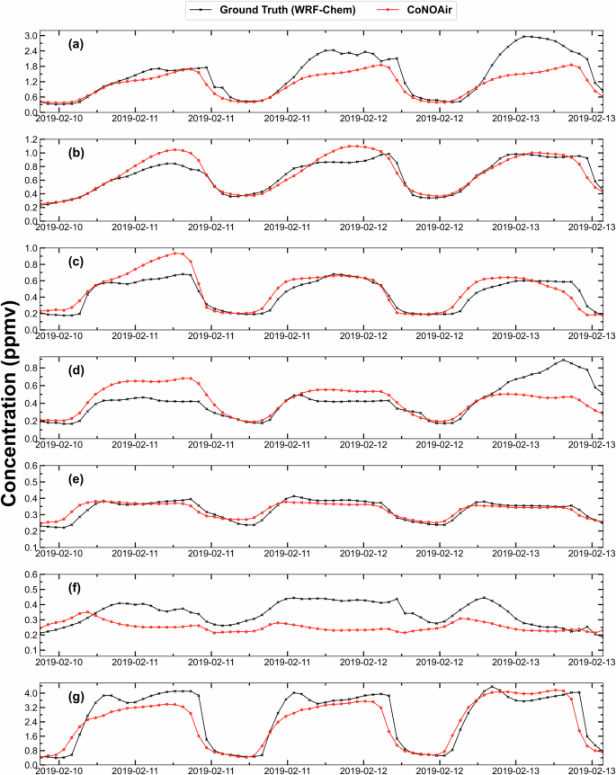
Figure 3 shows the performance of CoNOAir(4) over the six cities listed earlier and the maximum concentration grid point for short-term forecasts. Specifically, we focus on the next hour forecasting capability for the month of February 2019 (from the test set) for these locations. Interestingly, we observe that CoNOAir(4) captures the fluctuations, including the spurious ones with sudden increases, in CO concentration both quantitatively and qualitatively. To demonstrate this further, we analyse the parity plot of predicted with respect to ground truth CO concentrations for these locations (see Fig. 3). We observe that the R² values for all the locations are more than or equal to 0.95 suggesting a high accuracy in the prediction. From Supplementary Fig. 4, we can infer that the R² values for the seven grids for FNO(4) are less than or equal to CoNOAir(4). Supplementary Tables 2 and 3 suggest that CoNOAir(4) has the best performance both in terms of RMSE and MAE for every city and the maximum concentration grid point. The RMSE and MAE, even for the CoNOAir(16), are comparable to FNO(4). These results reinforce the superior performance of CoNOAir both in terms of short-term and extreme-value forecasting. Performance evaluation of WRF-Chem simulations with ground-based observation stations for these cities for the year 2019 can be found in the “Methods” section and Supplementary Material (Supplementary Table 4 and Supplementary Fig. 5).

**Fig. 3: Short-term forecast for Indian cities.**

Long-term forecasting

Long-term forecasting is an important aspect of pollution for strategic planning of the cities and policymaking. We now analyse the capability of CoNOAir to perform a reliable long-term forecast of CO concentration. Figure 4 shows one instance of 72 h forecast using CoNOAir(16) starting 10th February 2019 at 12:00 IST in an autoregressive fashion (see Supplementary Materials for the results of the remaining models, Supplementary Figs. 6–10). The ground truth and the corresponding prediction using CoNOAir for the 1st, 12th, 24th, 48th, 60th and 72nd-h forecasts are shown for comparison (see Fig. 4). We observe that CoNOAir can provide reasonable forecasts both qualitatively and quantitatively for the 72nd hour as well. Specifically, CoNOAir is able to reproduce the overall patterns of dispersion and the distribution of the CO concentrations over the country with sufficient accuracy. On a closer examination, CoNOAir appears to be underestimating the concentrations over the country on longer timescales. The selection of this timestamp, i.e., noon hour when the potential of the dispersion of pollution is high, also explains the ability of our proposed model to build over relatively lower concentrations autoregressively to determine the future concentrations. The evolution of error metrics over all samples is given in Supplementary Fig. 2(g–i).

**Fig. 4: Country-wide evolution of long-term forecast.**

Finally, we analyse the long-term forecast of CoNOAir(16) for the selected cities and the maximum concentration location for 72 h for the same instance as above (see Fig. 5). CoNOAir(16) performs reasonably well for all the cities except Dehradun where the concentrations of CO are low. This shows the model’s competence to efficiently replicate a greater range of concentration values autoregressively (Supplementary Table 5 depicts the RMSE for forecasting 72 h over these cities). It is impressive that the model’s performance over the maximum concentration grid point is reasonably accurate even for a 72nd-h forecast. This explains the superiority of the CoNOAir(16) model in forecasting CO levels at grids with high concentrations, that too autoregressively, making it a reliable model to be used for developing warning systems for predicting future episodes and preparing for them.

**Fig. 5: Grid-level evolution of long-term forecast.**

These rollout predictions can be made for timesteps beyond 72 h as well for every model. Supplementary Figs 11–16 show this. However, our previous experience suggests that errors accumulate for subsequent rollout predictions and 72 h becomes a longer period for the accumulation of errors⁵³. Further, previous studies⁵⁴ have highlighted the challenges in longer-term forecasting (24 h), ⁵⁵ predicted 48-h in advance for long-term hourly forecasting, while Chiang et al. ⁵⁶ have made predictions for 72 future timesteps. The latest study by Zhang et al. ⁵⁷ also developed ML models for hourly 3-days’ forecasts. Therefore, we have limited our analysis to 72 h rollout forecasts as long-term for relative comparison to the 1-h predictions, which is the shortest timescale for making predictions.

Discussion

Air quality modelling using ML algorithms can adeptly address challenges inherent in conventional models. This study advances ML models to simulate CO concentrations across India through operator learning. The operator learning approach for PDE inferencing offers the advantage of learning continuous functions using global convolution with Fourier transformation, whereas traditional DL methods employ local convolutions that are better suited to learning edges and shapes. DL methods are further limited by the discretization of data as they learn the mapping between finite-dimensional spaces. Neural operators, due to the usage of global convolution can produce resolution-invariant solutions for operators, whose parameters can be reused for different mesh sizes. Neural-FEM methods model one instance of a known PDE using a neural network, however, Neural Operator learns the solution operator without any information about the PDEs⁴⁹. Moreover, CoNOAir performed better for out-of-distribution data than FNO models proving that operator learning is a better approach to handle the problem of pollution prediction⁵¹.

We trained the existing FNO model and introduced an enhanced architecture, CoNOAir, utilising the fractional Fourier transform to better represent non-stationary signals and optimise parameters in complex space for learning the time evolution of the advection-diffusion equation. Training the FNO and CoNOAir models ranged from 4 to 80 h on a single NVIDIA V100 GPU with 32 GB memory (see Supplementary Note 3 for more information). Further, generating inferences with these ML models took mere seconds for 72-h forecasts, highlighting their potential to address computational time-related constraints of conventional models.

We evaluated the performances of three CoNOAir and FNO configurations based on short-term (1 h) and long-term (3 days) forecasting. CoNOAir configurations consistently outperformed their FNO counterparts, indicating that FNO would require more parameters to achieve a similar level of performance. Detailed performance analysis over six major cities and the location with the highest CO concentrations revealed that CoNOAir(4) excelled in one-hour forecasts, while CoNOAir(16) outperformed or matched FNO(16) across all grids for forecasting 72 h in an autoregressive fashion. CoNOAir has several architectural features that provide superior performance in comparison to FNO. One key feature of CoNOAir is the use of fractional FT (FrFT) in lieu of FFT, which provides both time and frequency representation. In contrast, FFT uses just frequency and hence, may perform poorly on non-stationary signals. FrFT can capture non-stationary signals (changes in signal characteristics with time) better than FFT and identify the instantaneous change in frequency better than FFT, a typical feature exhibited by our datasets. Additionally, CoNOAir utilises Complex-Valued Neural Networks to further improve the representation of input signals in terms of both magnitudes and phases, providing greater information for the model to learn. FFT has limited spatial granularity of the order (({n}log (n))) on a uniform grid and struggles to capture local variations. FrFT has a learnable parameter alpha to transform the input and preserve the information of the time variation of frequency in the input signal to capture local variations effectively.

The super-resolution capability of the operators allows predictions at multiple resolutions for the micromanagement of hotspots and cities, facilitating the development of advanced intervention strategies. Future directions include integrating physics and chemistry-based information for precise CO and other pollutant predictions and developing real-time early warning systems. This framework could potentially be scaled globally to forecast CO concentrations for any city worldwide, offering enhanced management scenarios and improving living standards.

It is imperative to discuss the limitations and future direction of the current work. The current methodology incorporates only past concentration over India as input to output future concentration, whereas the concentrations are a function of emissions, meteorology, terrain, and background concentrations for instance. This limits the ability of CoNOAir to forecast when these inputs face sudden variations. The inclusion of these input parameters would further constrain CoNOAir to learn the complex relationships between them and make it robust. Uncertainties in emission inventory and meteorological simulations during WRF-Chem simulations generate uncertainties in the training data. Including ground-based observation data from monitoring stations during model training can reduce uncertainties which is our future direction for this work.

Methods

Data generation and preprocessing

In this study, we used the Weather Research and Forecasting coupled with the chemistry module (WRF-Chem) model (v3.9.1) for simulating air pollutant concentrations from 2016 to 2019 across India. More details about the configuration and validation of WRF-Chem are available elsewhere and are only briefly discussed here^{25,58,59,60,61,62}. Simulations were performed at a spatial resolution of 25 × 25 km² comprising 140 × 124 grids covering India. Model for Ozone and Related Chemical tracers’ version 4 (MOZART-4) along with gas-phase chemistry coupled with Model for Simulating Aerosol Interactions and Chemistry (MOSAIC-4 bins) was employed. The boundary conditions for the chemical fields were taken from the Community Atmosphere Model with Chemistry (CAM-Chem) Global Chemical Transport Model at 6 h temporal resolution. The Emissions Database for Global Atmospheric Research (EDGARv5.0) was used for the anthropogenic emissions of various pollutants at a resolution of 0.1°. These emissions from 26 sectors were combined into 5 major sectors and scaling factors were applied on the base year 2015 for every sector for the subsequent years. The WRF-Chem output, generated in the form of a NetCDF file, was extracted as NumPy arrays and saved into *.mat file format for training the models. The ground-level CO concentrations (available at multiple elevation levels from WRF-Chem) as 2D arrays for the entire country with a temporal resolution of 1 h (considered as ground truth in this study) and the corresponding timestamp were extracted. Subsequently, for the purpose of training and validation, respective datasets were prepared using the concentrations simulated for the years 2016, 2017, and 2018. To generate the training and validation set, we used the moving window approach to generate smaller time series each of 26 h from the ground-truth data. All the samples were then shuffled randomly to obtain 3000 samples for training and 500 samples were obtained for testing the model’s performance during the training as validation set. The simulated data for the year 2019 was kept separately as a holdout (test) set to assess our models’ performances. The training, validation and test datasets were then normalised to the [0, 1] range using the absolute minimum and maximum values from the training dataset, considering both temporal and spatial dimensions to accelerate the training process.

Model architecture

A neural operator, CoNOAir is developed in this study to model CO concentrations and the performances are evaluated against the ground truth. Further, we compare the performance of CoNOAir with one of the most widely used neural operators, namely, FNO, which gives state-of-the-art performance in several problems related to the time evolution of partial differential equations^50,63,64. The problem formulation of the Neural Operator and its theory is presented subsequently.

Let ({rm{d}}in {mathbb{N}}{,}Omega in {{mathbb{R}}}^{{rm{d}}}) denotes bounded, open set with ({rm{A}}={rm{A}}left(Omega {;}{{mathbb{R}}}^{{{rm{d}}}_{{rm{a}}}}right)) and ({rm{U}}={rm{U}}left(Omega {;}{{mathbb{R}}}^{{{rm{d}}}_{{rm{u}}}}right)) denoting separable Banach spaces of functions, representing elements in ({{mathbb{R}}}^{{{rm{d}}}_{{rm{a}}}}) and ({{mathbb{R}}}^{{{rm{d}}}_{{rm{u}}}}), respectively. Suppose ({{rm{G}}}^{dagger}:{rm{A}}to {rm{U}}) represents the underlying non-linear surrogate mapping derived from a solution operator of parametric PDE. It is assumed that independent and identically distributed (i.i.d.) observations ({({{rm{a}}}_{{rm{j}}}{,}{rm{u}}_{{rm{j}}})}_{{rm{j}}=1}^{{rm{N}}}) are available, where ({{rm{a}}}_{{rm{j}}} sim {rm{mu }}) are sampled from the underlying probability measure ({rm{mu }}) supported on ({rm{A}}), and ({{rm{u}}}_{{rm{j}}}={{rm{G}}}^{dagger}({{rm{a}}}_{{rm{j}}})).

The aim of operator learning is to approximate ({G}^{dagger}) using a parametric mapping (G:Atimes varTheta to U) or equivalently, ({G}_{theta }:Ato U,,theta to varTheta), belongs to a finite-dimensional parameter space (varTheta). The objective is to identify(,{theta }^{dagger}in varTheta) such that (Gleft(.,{theta }^{dagger},right)=,{G}_{theta }^{dagger},approx {G}^{dagger}). It enables learning in infinite-dimensional spaces by solving the optimisation problem in Eq. 1 constructed with a loss function ({mathcal{L}}:Utimes U) ({{to}}{mathbb{R}}).

$$mathop{min }limits_{theta in varTheta }{E}_{a sim u}{mathcal{[}}{mathcal{L}}left(Gleft(a,theta right),,{G}^{dagger }left(aright)right)]$$

(1)

In neural operator learning, ({{rm{G}}}_{{rm{theta }}}) is parameterised using deep neural networks. Equation 1 is optimised using a data-driven approximation of the loss function. ({{rm{G}}}_{{rm{theta }}}) consists of three main components as follows:

a.

Lifting Operation (({rm{P}}:,{{mathbb{R}}}^{{{rm{d}}}_{{rm{a}}}}to ,{{mathbb{R}}}^{{{rm{v}}}_{0}})): projects input to high-dimensional latent space using a fully dense pointwise neural network along the channel dimension.
b.

Kernel Integration Operation (({rm{K}})): represented iterative kernel operation that maps through a series of linear operators and non-linear activation. It can be represented as follows:

$${V}_{l+1}=sigma (W{v}_{l}+{b}_{l}+{rm{K}}(a{;}phi){v}_{l})$$

(2)

where (it {{sigma }}) represents a non-linear activation function and (it {{phi }}) denotes the kernel parameterised using neural network and (it {{W}}) represents the bias term.
c.

Projection Operation (Ǫ: ({{mathbb{R}}}^{{{rm{v}}}_{{rm{t}}}}to ,{{mathbb{R}}}^{{{rm{d}}}_{{rm{u}}}}left)right.): projects high-dimensional latent space to output using a fully dense pointwise neural network along the channel dimension,

Overall, ({{rm{G}}}_{{rm{theta }}}) can be represented as follows:

(3)

where ∘ denotes the composition operation.

Kernel Integral Operator: For the iterative updates in neural operators, the linear transformation is represented by a nonlocal kernel integral operator. It can be characterised using a kernel function ({rm{kappa }}):

$${rm{K}}(a{;}phi ){v}_{l}(x)=mathop{int }limits_{D}kappa (x,y,aleft(xright),a(y){{;}phi )v}_{l}(y){rm{d}}y$$

(4)

This kernel integral operation is formulated as a convolution operation which becomes a multiplication operation in the Fourier Domain. Let ({mathcal{F}}) represent the Fourier transform:

$${rm{K}}(a{;}phi){v}_{l}(x)={{mathcal{F}}}^{-1}({mathcal{F}}({{kappa }}_{phi}){{.}}{mathcal{F}}({nu }_{l}))(x)$$

(5)

Hence, the FNO model parameterises the Fourier transform of this kernel function directly in Fourier space and the outputs are again converted to the spatial domain as follows:

$${rm{K}}(a{;}phi){v}_{l}(x)={{mathcal{F}}}^{-1}({R}_{phi}{{.}}{mathcal{F}}({nu}_{l}))(x)$$

(6)

In CoNOAir, the kernel integral is formulated using the Fractional Fourier Transform (FrFT) with a learnable order. The kernel integral is carried out within the complex-valued domain using Complex-Valued Neural Networks (CVNNs). Unlike, the FNO employs the Fourier Transform to handle the integral kernel with real-valued inputs and outputs. In CoNOAir, the integral kernel can be mathematically formulated as:

$${rm{K}}(a{;}phi){v}_{l}(x)={{mathcal{F}}}^{-alpha}({R}_{phi}.{{mathcal{F}}}^{alpha }({nu}_{l}))(x)$$

(7)

where ({{mathcal{F}}}^{{rm{alpha }}}) denotes the order ({rm{alpha }}) fractional Fourier transform and ({{mathcal{F}}}^{-{rm{alpha }}}) denotes inverse fractional Fourier transform. The kernel is parameterised as a learnable weight ({{rm{R}}}_{{rm{phi }}}in {rm{theta }}). In CoNOAir, ({rm{alpha }}) also becomes a learnable parameter.

Model training and hyperparameters

In this study, we used the variation of FNO, which performs convolution in the 2D spatial domain only and the input is fed into the model as a time series, just like a Recurrent Neural Network. A similar architecture for CoNOAir was used to compare their ability to make forecasts. The number of Fourier modes used was 12, with 20 hidden channels for each transformation unit. All the variations of these models were run for 500 epochs with an initial learning rate of 0.001 which was halved after every 100 epochs. RL² Norm, as given in Eq. 8, was used as the loss function with Adam as the optimiser.

$${rm{R}}{{rm{L}}}^{2},{rm{Norm}}=frac{sqrt{mathop{sum }nolimits_{u=,1}^{ntimes m}{left({Y}_{u}-widehat{{Y}_{u}}right)}^{2}}}{sqrt{mathop{sum}nolimits_{u=,1}^{ntimes m}{left({Y}_{u}right)}^{2}}}$$

(8)

({{rm{Y}}}_{{rm{u}}}) is Ground Truth (WRF-Chem) and ({hat{{rm{Y}}}}_{{rm{u}}}) is Predicted Value (FNO or CoNOAir). ({rm{n}}times {rm{m}}) represents the total number of grids after converting it into a 1D vector.

For our ablation studies, we used 8, 10, 12 and 16 previous timesteps as inputs to our models, from which we concluded that 10 and 12 configurations worked the best. Finally, we selected the configuration of utilising 10 previous timesteps as inputs to predict one timestep at a time. Subsequently, we can use the forward pass in an autoregressive fashion to output the required number of future steps. To update the models’ parameters during the backpropagation of loss, we calculated the cumulative loss over the autoregressive forecasting for 4, 6 and 16 timesteps. The rationale behind this step was to develop models for both short-term and long-term forecasting by accumulating losses over smaller and longer time frames and to compare their abilities to make forecasts on both timescales. We established a uniform nomenclature for the rest of the paper to identify the different configurations of the models trained in this study. The name will be a combination of the type of architecture employed, whether it is CoNOAir or FNO and the number of timesteps (4, 6, or 16) used to propagate the loss backwards. For example, FNO(6) will represent the FNO architecture where 6-step forecasts were used to propagate the loss backwards and so on.

Model evaluation metrics

To evaluate our models’ performance over short-term forecasting as well as long-term forecasting we have chosen three commonly used metrics namely Root Mean Squared Error (RMSE), Mean Absolute Error (MAE) and RL² Norm. We calculated the RMSE, MAE and RL² Norm between every predicted and corresponding observed image pair over all the samples and compared the mean and standard deviations. To calculate every metric, we converted the 2D arrays into 1D vectors and performed the respective operations. RMSE between one observed and predicted image was calculated as given in Eq. 9 follows

$${rm{RMSE}}=sqrt{frac{1}{ntimes m}times mathop{sum}limits_{u=1}^{ntimes m}{({Y}_{u}-widehat{{Y}_{u}})}^{2}}$$

(9)

Similarly, MAE and RL² Norm were calculated as shown in Eqs. 10 and 8, respectively.

$${rm{MAE}}=frac{1}{ntimes m}times mathop{sum}limits_{u=1}^{ntimes m}{|}{Y}_{u}-widehat{{Y}_{u}}{|}$$

(10)

where RMSE is Root Mean Squared Error, MAE is Mean Absolute Error, ({{rm{Y}}}_{{rm{u}}}) is Ground Truth (WRF-Chem) and ({hat{{rm{Y}}}}_{{rm{u}}}) is Predicted Value (FNO or CoNOAir). n (times) m represents the total number of grids after converting it into a 1D vector.

In this study, we have evaluated our models’ performance on the test data that was used for the validation during the training process, which comes from a similar distribution as the training data. Subsequently, we tested our models on out-of-sample data which comes from the observed data of the 2019 year. For the test data, we forecasted in an autoregressive fashion for the next 16 h and obtained the mean and standard deviation of the metrics defined above corresponding to every timestep’s forecast. Similarly, for the whole out-of-sample data we have made forecasts for the next 20 h. We also took 168 samples spanning over an entire week from the month of February 2019 to evaluate our models’ capacity to forecast longer timeframes, i.e., the next 72 h over the entire country whose results are shown in Table 1, and Supplementary Fig. 2. We further analysed the short-term forecasting ability, i.e. the next one hour, of our models on the grids representing the six cities listed previously, along with the maximum concentration grid point. For this evaluation, we have used the R² metric, RMSE and MAE to compare our model performance. The complete results are shown in Fig. 3, Supplementary Fig. 4, Supplementary Tables 2 and 3.

We also analysed the comparison between the time-series evolution for 72 h using autoregressive forecasting with observed time series for these 7 grid locations, whose results are shown in Fig. 5 and Supplementary Table 5. Finally, we assessed our models’ performance for the worst CO concentration events obtained using cumulative maximum concentration for the three crucial hours (i) morning rush, (ii) evening rush and (iii) midnight inversion illustrated in Fig. 2 and Supplementary Fig. 3.

Validation of WRF-Chem simulations with ground-based observation data

We obtained the AQ data available from the Central Pollution Control Board’s monitoring stations corresponding to the grids representing Delhi, Mumbai, Guwahati, Bengaluru and Ahmedabad for 2019, the year for which our models are evaluated. We averaged the data from all the stations wherever multiple stations were available in the grid for comparison. Delhi had 16 stations, Mumbai had 5 stations, Bengaluru had 4 stations and Ahmedabad and Guwahati had 1 station each. There was no station data for Dehradun and max concentration grid point for this year. The metrics for the evaluation of performance for each city (Mean Bias, Root Mean Squared Error) are shown in Supplementary Table 4 and time-series plots are shown in Supplementary Fig. 5.