A rapid run-out assessment methodology for the 2024 Wayanad debris flow
Introduction
Debris flow activity is highly prevalent in the Western Ghats (WG) (Fig. 1a) due to steep topography and intense monsoon rainfall, particularly in the highlands of Kerala1,2,3. The southwest and northeast monsoon systems lead to heavy, prolonged rainfall4, which significantly contributes to the occurrence of rain-induced debris flows in this region5. On 30th July 2024, around 1.30 am, Wayanad district in Kerala, India, reported a massive debris flow, which resulted in nearly 231 deaths and 128 people missing, much beyond the median value of 165 deaths worldwide annually by debris flow6,7,8. This event originated in a densely vegetated area at an elevation of ~1620 m above mean sea level (amsl) in the headwater of the Chaliyar River (11°27’57.07”N, 76°8’9.91”E). The initiation of debris flow overlaps with the high landslide susceptible zone in the Geographic Information System-Tool for Infinite Slope Stability Analysis (GIS-TISSA) map9 (Fig. 1b) (Methods). This massive debris flow swept through a valley (Supplementary Figure 1) in the WG, devastating Punchirimattom, Mundakkai, and Chooralmala villages throughout a distance of 8 km, over a significant elevation difference of 768 m (Fig. 1c). The crown of the debris flow is superimposed on the scar of an old bigger landslide that occurred on 1st July 1984, killing 14 people, triggered by 340 mm rainfall in 24 h, and another smaller event in 2019–20, indicating frequent debris flow activity of this region to rain-induced soil saturated condition10. Additionally, the debris flow location is nearby the previously occurred long run-out Kurichermala (30 km) and Puthumala (3 km) landslides (Supplementary Figure 2). According to the data from the Kalladi rain gauge of the Irrigation Design and Research Board (IDRB) (5 km away from the debris flow location; 11°30’30”N, 76°07’43”E), the region received 572.8 mm of cumulative rainfall in 48 hours, with 372.6 mm of rainfall on 30th July 2024 (Supplementary Fig. 3).
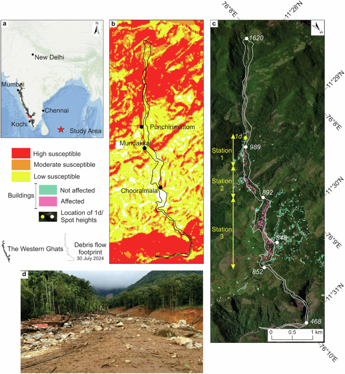
a The Western Ghats with the study area marked (b) Delineated footprint of the debris flow overlaid with landslide susceptibility map (c) Distribution of buildings in and around the delineated footprint of debris flow (d) Distant view of debris flow scarp and its flow path (Background image: (a) ArcGIS base map; (b) GIS-TISSA; (c) Google Earth).
Immediately after this debris flow, technologies such as ground penetrating radar (GPR), thermal scanners and unmanned aerial vehicle (UAV) were promptly implemented for rescue and rehabilitation, prioritizing the evacuation of the stranded population as well as the search for the missing. However, scientific investigations for reconstructing the determinants behind such large-scale debris flow are crucial for improving management practices and mitigation strategies for imminent debris flow. Obtaining the precise footprint of the debris flow immediately after the event can be challenging, often requiring waiting for the next available cloud-free satellite image. Here, we introduce a methodology to identify the characteristics and extent of devastation in a short-time period using the immediately available crowd-sourced data and RApid Mass Movement Simulation (RAMMS) (Methods and Supplementary Figure 4) for scientific studies as well as for rescue operations.
Observation and modelling
Based on the available post-event drone video, media photos and Google Earth images, the flow path was digitized. Tree heights within the tropical rainforest, observed in the drone video of the affected area, were used as a reference to estimate the vertical extent of material displaced, and through that a release depth of 10 m was assigned. Our simulation results employing RAMMS show a maximum flow height (MFH) of 5 m for the debris flow, a maximum flow velocity (MFV) of 5.5 m/s, and a maximum flow pressure (MFP) of 61.4 kPa at station 1 (Punchirimattom village, located 2.5 km downstream of the scarp at an elevation of 1000 m, and affecting an area of 0.4 km2 by a flow volume of 5.3 x 10⁵ m3) impacting 73 buildings (Fig. 2). At station 2 (Mundakkai village with 0.25 km2 affected area and flow volume of 3.1 x 10⁵ m3), MFH was 5 m, MFV was 6.6 m/s and MFP was 88 kPa affecting 61 buildings. Near station 3 (Chooralmala village with 0.94 km2 area and flow volume of 3.8 x 10⁵ m3), MFH of 4.5 m, MFV of 4.68 m/s and MFP of 43.8 kPa was estimated, affecting 293 buildings including schools and a bridge connecting the villages. The study identified 1018 building footprints in the area, with the simulation indicating that 427 houses were damaged. This number is close to the actual values reported in the media11.
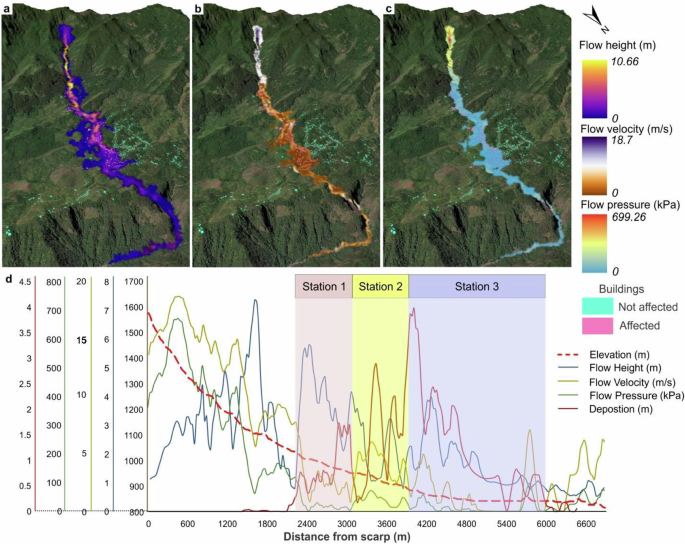
a Flow height (m) (b) Flow velocity (m/s) (c) Flow pressure (kPa) (d) Profile of flow characteristics and elevation along the central thalweg of the debris flow path (Software: RAMMS::Debris Flow; Background image: (a–c) Google Earth).
Run-out modelling showed that the debris flow attained its maximum velocity (18.27 m/s) and pressure (668 kPa) at a distance of 0.5 km away from the scarp zone. A maximum flow height of 7.3 m was achieved when the debris mass was 1.6 km downstream of the scarp (Fig. 2a–c). Furthermore, a deposition thickness of ~4 m was observed at 4 km downstream from the source (within station 3), highlighting significant sediment accumulation and run-up height, causing severe devastation. The greater velocity in the initial phase can be attributed to terrain gradient, channel morphology, material properties and initial trigger. The maximum height at midway can be ascribed to the sudden decrease in slope as well as the presence of narrow valley that caused severe inundation and continuous accumulation of material, including large boulders. The final deposition can be due to changes in gradient and impediments to velocity by successive impacts on buildings. Based on these observations, the settlements at these stations were identified as being at high-risk due to their proximity to the stream, which attained high velocities during the storm. These findings provide a comprehensive understanding of the debris flow’s destructive behavior and its impact along the flow path.
Implications
Analysis along the central thalweg of the debris flow path reveals critical points of material accumulation, velocity, and pressure (Fig. 2a–d). Significant deposition at lower elevations, as shown in the simulation (Fig. 2) and validated using post-event images (Supplementary Fig. 5), indicates transient changes in the landscape and potential downstream hazards posed by sediment disasters. The maximum velocity and pressure values down the scarp highlight zones of intense dynamic activity, which are crucial for understanding the force and impact of the debris flow. These insights are vital for designing effective mitigation and monitoring strategies in similar terrains. Run-out modelling shows potential areas of significant destruction downstream from high-susceptibility zones (Fig. 1b). This underscores the importance of detailed vulnerability mapping, especially in areas characterized by highly fluidized debris flow, by incorporating potential run-out zones. By avoiding habitation in identified debris flow-prone areas, including the run-out paths, communities can reduce the risk of future disasters and enhance their overall safety. Thus, creation of advanced susceptibility maps by incorporating run-out paths is a pre-requisite. Development of early warning systems to enhance future mitigation and planning efforts are critical in this region to save lives12, with measures such as extensive rainfall and soil moisture monitoring stations to create thresholds. Additionally, proper land-use planning is essential to reduce the impact of such destructive debris flows. We also recommend mapping high-risk zones near the first- and second-order streams in steep slope regions, and providing sufficient offsets or avoiding settlements. Thus, given its severe impact and high run-out velocities, this debris flow highlights the urgent need for improved disaster management in the WG. Additionally, this disaster emphasizes the value of simulation and crowd-sourced data for damage assessment and planning, shortly after the event. Such scientific documentation, immediately after an event, is quintessential for mitigating any imminent landslides, which are usually not done but can be alternatively overcome using the method mentioned in this study.
Thus, the current study presents a novel approach by using run-out modelling to analyze one of the largest and most destructive debris flows in India. This study was successful in capturing field observations through remote sensing and media information to provide preliminary modelling assessments. This would be useful to serve as a foundation for more detailed models once field observations are available. It helps to establish baseline parameters, which can be updated and expanded later to assess future risks more comprehensively. Furthermore, such preliminary modelling has the potential to inform the recovery process, as well as the immediate post-event safety and infrastructure evaluation.
Methods
Debris flow simulation
In the study area, buildings were digitized using high-resolution Google Earth imagery, and further analyses were conducted in a GIS environment. Specific landmarks such as settlements, schools, bridges, temples and mosques identified from drone footage along with post-event photographs, were marked on Google Earth. These reference points were used to georeference the images and establish the boundary conditions of the debris flow path. The extent of the debris flow was then identified, and the derived footprint was used to simulate the run-out using RAMMS::Debris flow, which is commonly used for simulating debris flows in mountainous regions due to its ability to account for complex terrain and its use of Voellmy rheology to model flow dynamics and frictional behavior13,14. The required input for RAMMS is topographic data (pre-event DEM) in GEOTIFF format, for which the 30 m resolution Shuttle Radar Topography Mission (SRTM) elevation data (Supplementary Table 1) was used. As the debris flow followed the stream channel, the input hydrograph was defined as the starting condition, with an initial hydrograph volume of 860,000 m3 and hydrograph peak discharge time (t1) = 40 s. The delineated footprint’s depletion part was defined as the release area in RAMMS, with a release depth of 10 m, identified from drone footage of the debris flow source. The hydrograph volume was calculated by multiplying the release area by the release depth. Applying this volume estimate, RAMMS used Rickenmann’s15 empirical relationship to determine the peak discharge and total discharge time. The friction coefficients were calibrated using a trial-and-error approach based on values from the literature. The velocity independent dry-Coulomb type friction coefficient (μ) represents the internal properties of the flow, like shear strength, affecting the run-out distance16. The velocity dependent viscous-turbulent friction coefficient (ξ) was adjusted to account for turbulent flow characteristics, particularly for muddy flows exhibiting larger ξ values17. After several simulations, μ = 0.1 and ξ = 600 m/s2 were selected to ensure that the modelled flow path matched the boundaries observed in post-event photographs (Supplementary Figure 5). RAMMS simulated the flow along the terrain, providing flow characteristics such as flow height, flow velocity, flow pressure, and deposition. To analyze these flow characteristics, three clusters of settlements: Punchirimattom, Mundakkai, and Chooralmala that were severely impacted by the debris flow were considered as the three stations. The adopted methodology is illustrated in a two-stage flow chart, shown in Supplementary Figure 4.
Sensitivity analysis of RAMMS input parameters
Sensitivity analysis of friction parameters in RAMMS14 highlights that both μ and ξ significantly influence debris flow modeling outcomes. An overview on the various studies found that typical values for μ range widely between 0.05 and 0.5, most commonly around 0.1 or 0.2, while ξ value ranges between 10 and 2000 m/s2. These friction parameters are adjusted to match local debris flow characteristics, such as slope, material type, and hydrological conditions. The input parameters including ξ, μ, release depth and t1 were analyzed for their sensitivity.
Sensitivity analysis conducted along various points on the debris flow path of Wayanad reveals that the release depth demonstrated the greatest sensitivity in influencing flow height, with variations up to +/−50% producing substantial changes, affirming its crucial role in determining volume along the path. μ and ξ showed considerable sensitivity for both flow height and velocity, with μ and ξ values calibrated at 0.1 and 600, respectively, to provide a balanced response in the simulation. Additionally, t1 exhibited minimal sensitivity, indicating that temporal adjustments in the peak discharge calibrated at 40 s, have limited impact on overall flow characteristics, supporting this choice as an effective baseline. These findings justify the calibrated parameters as optimal, providing accurate simulation while reflecting the observed physical properties along the debris flow path.
Creation of landslide susceptibility map
GIS-TISSA9 is a python-based implementation of the Probabilistic Infinite Slope Analysis (PISA-m) algorithms through the First-Order Second-Moment (FOSM) method18,19. It offers a graphical user interface (GUI) fully integrated within a GIS framework, allowing seamless interaction with spatial data. The creation of landslide susceptibility maps using GIS-TISSA relies on integrating digital elevation model (DEM), soil, and vegetation data, converted to raster format for pixel-based analysis. It calculates slope stability using the PISA-m or ArcMap slope method, with inputs for soil and vegetation types from .csv files. The algorithm computes the factor of safety (FS), probability of failure (FS < 1) and reliability index (RI), saving these as raster outputs9. The high-, moderate- and low-susceptible zones were classified from the output raster of FS.
Creation of geomorphological map
Geomorphological map was prepared using the r.param.scale module in GRASS GIS20, which extracts terrain parameters from the DEM by fitting a bivariate quadratic polynomial to different window sizes. This multi-scale approach allowed us to identify morphometric features such as peaks, ridges, passes, channels, pits, and plains, providing a detailed geomorphological representation of the region. The delineated footprint is overlaid over the geomorphological map for identifying the morphometric features along the flow path (Supplementary Figure 1).
Comparison of RAMMS simulation with the real debris flow footprint
The real footprint of the debris flow was digitized using PlanetLab image, acquired on 12th August 2024, which is the immediate cloud-free post-event imagery. The flow height simulated by RAMMS is compared with the real footprint to estimate the accuracy of the flow path predictions by RAMMS (Supplementary Fig. 6). From the analysis, RAMMS have predicted 96% of the actual flow path, aligning closely over the boundaries in the impacted areas such as station 1 and 2, while over-predicting 85%. This over-prediction could be due to the coarse resolution of the SRTM elevation data used for the simulation. This could be improved by using a high resolution pre-event DEM for the simulation. The under-prediction is only 4%, which highlights that the simulation could predict the majority of the flow path, only leaving the least percentage unpredicted. The study has predicted devastation of 427 buildings, which was the true count, with no structures missed by the predicted flow path.
Responses