A system-level model reveals that transcriptional stochasticity is required for hematopoietic stem cell differentiation

Hematopoiesis is the process that leads to the production of all blood cell types from a single precursor known as Hematopoietic Stem Cell (HSC)¹. HSCs reside in the red bone marrow, specifically within a hypoxic niche shaped by various native bone marrow cells, including stromal cells, macrophages, adipocytes, osteoblasts, osteoclasts, and endothelial cells (Fig. 1a)². Hematopoietic stem cell niche (HSCN) processes are influenced by the secretion of cytokines, chemokines, and metabolites such as ATP and fatty acids³. At the spatial level, it has been reported that HSCs found deeper in the HSCN remain mainly quiescent and metabolically dependent on glycolysis, while HSCs close to the edge of the niche have higher proliferative potential⁴. Quiescent HSCs exit this cell state to self-renew and to produce other common progenitors with specific lineage commitment capacities: megakaryocyte-erythroid progenitors (MEPs), common myeloid progenitors (CMPs), granulocyte-monocyte progenitors (GMPs), and common lymphoid progenitors (CLPs), all of which will differentiate into all blood cell types⁵ (Fig. 1b). As differentiation begins, HSCs switch their ATP source from glycolysis to oxidative phosphorylation (OXPHOS) and increase both the concentration of reactive oxygen species (ROS) and their cell cycle rate^6,7,8.

a Anatomical schematization of the HSCN. b Deterministic differentiation of HSCs. c Classical model of hematopoiesis, in which multipotent cells are transcriptionally homogeneous and lineage commitment is a hierarchical stepwise process with cells gradually losing differentiation potential. d Revised hematopoietic model establishes transcriptional heterogeneity of HSCs and early lineage commitment.

Full size image

During normal hematopoiesis, common progenitor frequencies are tightly controlled in order to produce the correct amount of every cell type. This process has been explained using conceptual models of cell differentiation, such as Waddington’s epigenetic landscape^9,10, which postulates that a multipotent progenitor can give rise to phenotypes with less differentiation potential, until reaching terminal stable cell fates. In consequence, HSCs differentiation has been depicted as a stepwise, hierarchical process involving the formation of intermediate cell types with multilineage differentiation potential, which is gradually reduced as differentiation proceeds¹¹ (Fig. 1c). Nevertheless, single-cell expression data have revealed significant heterogeneity in the transcriptional expression patterns of HSCs, indicating strong lineage commitment at very early stages of hematopoiesis^12,13,14,15. This suggests that a differentiation intermediate may exhibit multiple gene expression patterns without losing the direction of its cell fate^13,14,15. These data have challenged the existence of intermediate oligopotent cells, and the tree-like scheme of hematopoiesis¹³. Instead, a new paradigm has emerged depicting hematopoiesis as a continuum process of early lineage commitment^13,16,17,18 (Fig. 1d). However, the source of HSC heterogeneity and how it influences lineage commitment is still poorly understood¹⁸.

In this context, physiological factors that influence HSCN, such as oxygen levels, nutrient balance, ROS presence, cell-to-cell contacts, and paracrine signaling of constitutive bone marrow cells, may be responsible for inducing the heterogenic activation of transcription factors that initiate differentiation pathways of HSCs^{19,20,21,22,23,24,25}. Recent evidence suggests that this hypothesis is correct since it was observed in vivo that cells located in more superficial regions of the niche present a greater number of polymorphisms, which consequently increases the gene diversity of cells produced by hematopoiesis²⁶. For this reason, it is essential to study the dynamics of the HSCN and understand how these dynamics change in the presence or absence of several of these factors. However, exploring the differentiation dynamics of the HSCN is challenging; reproducing the optimal experimental conditions to explore the differentiation dynamics of the HSCN is unfeasible with in vitro assays and impractical with in vivo protocols where perturbation analyses are difficult to implement and often result in lethal phenotypes²⁷. Thus, using in silico assays based on computational modeling and data science approaches offers an alternative to analyze the dynamic behavior of the system, complementing in vitro and in vivo analyses.

With the advent of high-throughput technologies, protocols have been developed to statistically infer gene regulatory networks (GRNs) from expression data. However, these approaches present a high rate of false-positive predicted regulatory interactions and are unable to accurately resolve the details of regulatory motifs, the resulting dynamics, and the complex transcriptional logic of the underlying networks²⁸. On the other hand, experimentally grounded discrete Boolean models using bottom-up approaches have proven useful for integrating detailed experimental information into tractable dynamical models that can be analyzed to study the behavior of GRNs^29,30,31,32. Additionally, Boolean models can incorporate non-transcriptional regulatory interactions, such as phosphorylation and ROS oxidation, which are typically excluded from GRN inference methods that rely solely on top-down approaches based on transcriptional data. In the past years, various discrete models have been used to explain CMPs and CLPs cell specification and differentiation, CD4⁺ T lymphocyte plasticity, and the interaction between the microenvironment and cell communication networks in acute myeloid leukemia^{29,31,32,33,34}. These modeling efforts focus on the later stages of hematopoietic differentiation, while the complex dynamics of the initial steps of this developmental process remain to be uncovered.

In this study, we developed a 200-node GRN for early hematopoiesis grounded on experimental data. Since this network is too large for further computational analyses, we used GINSIM³⁵ to collapse the linear pathways of this large network, resulting in a 21-node network or complex regulatory core that retained functional feedback loops, which determine the network’s attractors³⁶. The 21-node network considers the interplay between key transcription factors involved in cell fate decisions, the influence of oxygen and ROS levels from the HSCN microenvironment, cell signaling regulators, as well as the internal metabolic state. Our goal is to mechanistically explain the role of these factors in the transition from stemness to differentiation during hematopoiesis. We used our network to implement Boolean, continuous, and stochastic mathematical models to analyze the early stages of hematopoiesis. Our models were able to reproduce ex vivo RNA-seq expression patterns of HSCs, MEPs, and GMPs. The models suggest that the size of the cell pool in each hematopoietic compartment is influenced by the regulatory network of HSCs differentiation and by transitions between the different common progenitors. Additionally, our models show that cell heterogeneity is relevant for proper HSC differentiation and recovery of complex patterns of transitions that have been documented among HSC types. Moreover, they also showed that the presence of oxygen at the HSCN increases differentiation and reduces the pool of quiescent HSCs. Finally, the models predict that such conditions occur due to intracellular augmentation of ROS production, altering metabolism and signaling of HSCs.

The gene regulatory network of HSCs

As a result of our manual search for experimental information on the processes regulating HSCs differentiation, we integrated an interaction network of 200 nodes (Supplementary Data 1). We reduced this network by using a network reduction algorithm implemented in GINSIM³⁵ into a 21-node GRN of HSCs that encompasses gene expression, signaling, and metabolism of HSCs (Fig. 2 and Supplementary Note 1). GINSIM collapses linear pathways, while retaining feedback loops, which are critical for the dynamics of the network and the emergent attractors^36,37. Concerning transcriptional regulation, the GRN of HSCs includes the following transcription factors: HIF-1, FOXO3, p53, Runx1, Meis1, Mef2c, CEBPA, GATA1, GATA2, PU.1, Ikzf1, and Gfi1. It has been reported that HIF-1 regulates the quiescence of HSCs as well as ROS homeostasis and metabolic adaptation to the hypoxic conditions of the HSCN³⁸. On the other hand, FOXO3 is important to sustain the regenerative properties of HSCs, since the loss of function of this protein decreases the self-regeneration of these cell types^1,39. In this sense, FOXO3 is also implicated with p53 in the maintaining of HSCs’ quiescence as well as regulation of ROS intracellular levels^1,39. Selective repression of GATA1, GATA2, and PU.1 conditions the progression in the differentiation pathway of HSCs towards MEPs and GMPs cell types^40,41,42,43. Furthermore, CLPs differentiation is controlled by Ikzf1 and Gfi-1⁴⁴. Similarly, it has been observed that the differential expression of p53³⁹, Gfi1⁴⁵, PU.1⁴⁶, and GATA1⁴⁷ directly affects lymphopoiesis, either increasing or reducing its speed.

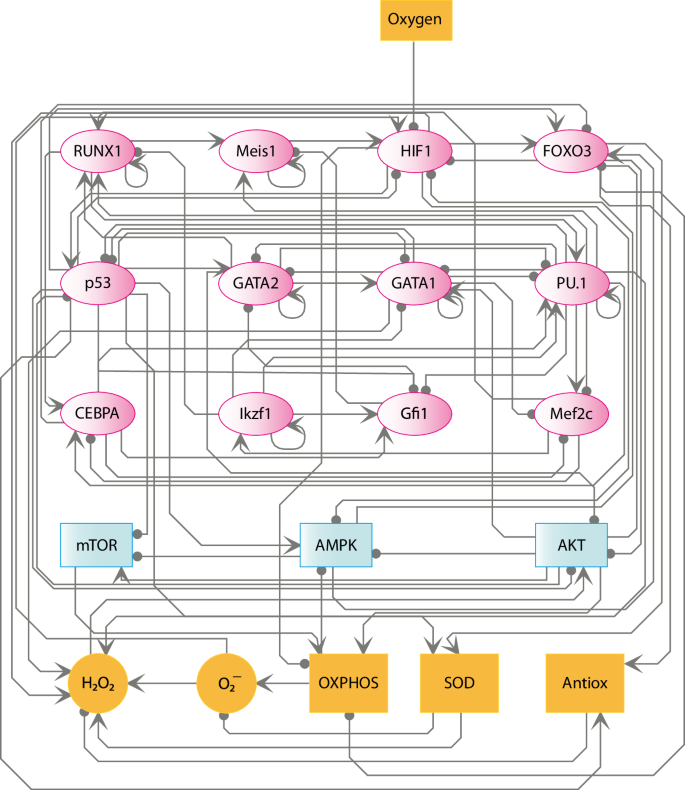
Topology of the GRN of HSCs differentiation. Transcription factors are represented as pink ellipses; blue rectangles represent signaling molecules; yellow circles represent ROS molecules, while enzymes and complex nodes are represented as yellow rectangles. Arrows indicate activating regulatory interactions, whereas inhibitions are represented with a line ending in a circle. Oxygen is the only input of this network.

Full size image

Experimental evidence shows that metabolic factors are essential to alter gene expression patterns that control HSCs differentiation^48,49. Indeed, these cells show a glycolysis-based metabolism, whereas differentiation of such cells shifts towards an oxidative metabolism in order to fulfill cellular energetic demands⁵⁰. To be precise, it has been seen that AMPK⁵¹, AKT⁵², and mTOR⁵³ exert critical functions in the regulation of the metabolic switch necessary to initiate the differentiation of HSCs. On the other hand, OXPHOS is one of the processes strongly regulated by the metabolic switch that controls the HSCs differentiation⁵⁴. This occurs because OXPHOS is a constant source of chemical energy in the form of ATP and ROS⁵⁵, which are suppressed by enzymes such as superoxide dismutase (SOD)²³ and catalases⁵⁶. Consequently, in this model, we represented as nodes the enzymes AKT, AMPK, mTOR, and SOD, as well as OXPHOS and ROS in the form of hydrogen peroxide (H₂O₂) and the superoxide ion (O₂^·−). The Antiox and Oxygen nodes represent the cellular ROS scavenger system and the oxygen concentration in the HSCN, respectively. Collectively, the nodes that compose this GRN (Fig. 2) represent fundamental molecules that regulate the differentiation of HSCs.

The network conditions the differentiation dynamics of HSCs

Boolean formalisms were used to represent and computationally study all interactions described by the GRN of HSCs (Fig. 2 and Table 1). The dynamic system can be explored either synchronously, that is, all nodes are updated at the same time, or asynchronously, where every node is updated independently. Under a synchronous updating scheme, the model identified 13 fixed-point attractors, which correspond to HSC, MEP, GMP, and CLP cell types, along with 5 cyclic attractors exhibiting mixed lineages markers (see Supplementary Figs. 1 and 2). When the more realistic asynchronous updating scheme was applied, only the 13 fixed-point attractors were recovered (Fig. 3). Fixed-point attractors are associated with robust, stable, and well-defined phenotypes, whereas cyclic attractors are linked to patterns of molecular activations that are unlikely to correspond to stable phenotypes^57,58. Therefore, further analyses were conducted considering only the 13 fixed-point attractors.

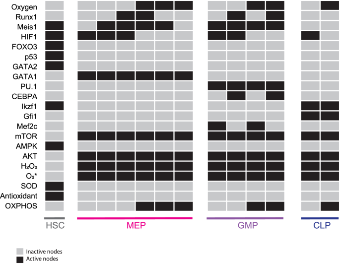
All possible initial states converge into 13 steady states that can be assigned to HSC (1 state), MEP (6 states), GMP (4 states), and CLP (2 states) lineages. Black boxes indicate that the corresponding node is active, while gray ones represent inactivity.

Full size image

The MEP, GMP, and CLP attractors show mTOR, AKT, and H₂O₂ activity as expected from active common progenitors^24,53,59,60. Additionally, MEP steady states show expression of the lineage marker GATA1⁶¹. GMP attractors are characterized by PU.1⁶² expression, while CLP steady states exhibit Gfi1 activity⁶³. Concerning HSCs, the model predicted that such cells present high expression levels of GATA2⁶⁴, FOXO3¹, p53³⁹, and Meis1⁶⁵, as well as high activity of AMPK⁶⁶ and low levels of ROS²⁴. Furthermore, this latter cell state can only be reached in the absence of Oxygen, as has been previously reported⁵.

RNA-seq datasets validate the GRN model

To validate the proposed Boolean network model, we evaluated its ability to reproduce the gene expression patterns observed in the cell types studied. To this end, we sought RNA-seq data on wild-type (WT) gene expression of the HSCs, MEPs, GMPs, and CLPs phenotypes. As a result of the search, we only found data for the HSC (accession number: GSE213596)⁶⁷, MEP (accession number: GSE112692)⁶⁸, and GMP (accession number: GSE88982)⁶⁹ phenotypes. Subsequently, the data were processed and discretized into two values (0 and 1) to compare them directly with the attractors recovered by the network (see Methods). It should be noted that to determine if there was OXPHOS activity, we used the Atp6v0b gene as a marker since it encodes a portion of the V0 domain of vacuolar ATPase⁷⁰, and it has been reported that its expression increases proportionally with OXPHOS activity⁷¹. At the end of this procedure, we found that the gene expression patterns predicted by the Boolean model under normal conditions strongly coincide with the actual patterns obtained using RNA-seq data (Fig. 4). However, our model exhibits some discrepancies with respect to the discretized RNA-seq data, some of which may be attributed to the discretization process of continuous gene expression. This process establishes a threshold above which a gene is considered expressed, while it is considered not expressed if its expression value falls below such threshold. Setting a threshold value is particularly challenging for transcription factors, whose expression levels are often lower than those of other transcripts⁷². For instance, in vivo studies report Ikzf1 expression in HSCs, GMPs, and CLPs compartments; with the highest expression in CLPs, where it plays a crucial role in establishing CLP identity⁷³. In the discretized RNA-seq data, Ikzf1 is only expressed in CLPs, whereas our model shows Ikzf1 activity in both HSC and CLP, consistent with in vivo experimental observations. Among the common progenitors, Mef2c expression is more conspicuous in CLPs⁷⁴ where it controls B and T cell specifications. Unexpectedly, in our model, Mef2c activity is not present at CLP attractors, suggesting that regulatory interactions are missing to restrict its activity to CLPs.

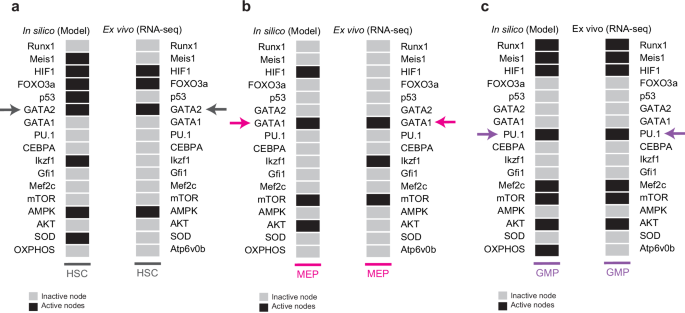
a Predicted gene expression pattern corresponding to HSCs vs. discretized RNA-seq data⁶⁷. b Boolean prediction equivalent to MEPs compared to discretized RNA-seq data⁶⁸. c Predicted attractors corresponding to GMPs compared to discretized RNA-seq data⁶⁹. Color arrows indicate the genetic markers used to distinguish each lineage. In this figure, OXPHOS is marked by the levels of the Atp6v0b gene.

Full size image

Biological networks have been shown to be robust systems in the face of perturbations. That is, they can maintain functionality and unchanged stable states in the face of mutations or external perturbations^75,76,77. A Boolean network can be perturbed either structurally, by altering its logical functions, or dynamically, by altering its trajectories⁷⁸. To further validate the proposed regulatory core, we assessed the robustness of our network against structural perturbations by randomly modifying the Boolean functions and measuring the percentage of original attractors recovered after such perturbations. Our network proved to be significantly more robust than random networks of the same size, under this type of perturbation (Supplementary Fig. 3). To assess the dynamic robustness of our model, we introduced random bit flips into the network states and evaluated their impact on the state trajectory. Robustness was measured by the Hamming distance between the original and perturbed trajectories. A lower Hamming distance indicates greater robustness, as it reflects a minimal deviation from the original trajectory⁷⁸. When compared to a thousand random networks of the same size, our network was more robust to dynamic perturbations (Supplementary Fig. 3).

The above simulations and results demonstrate that the model exhibits fundamental characteristics of biological networks, as it is robust against both structural and dynamic perturbations. Furthermore, its dynamic behavior aligns with current knowledge of gene expression patterns and the intracellular activity associated with HSC differentiation.

A systems-level approach to studying hematopoiesis solves experimental discrepancies

The standard validation procedure of Boolean models is achieved by recovering observed attractors in simulated mutations^31,32,79,80. This procedure evaluates the predictive ability of the model through a series of gain-of-function (GOF) and loss-of-function (LOF) mutation tests. To this end, information was sought on the effect of mutations on the differentiation of HSCs. Next, we performed simulations to recreate the conditions described in the literature, using both synchronous (Supplementary Figs. 4–90) and asynchronous (Supplementary Figs. 91–132) updating schemes, and determined the impact of these alterations on the model (see “Methods”).

We used the size of the basin of attraction as an indicator of the magnitude of the phenotypic population (Supplementary Tables 1–44). In the WT system, the normalized sizes of the basins of attraction for HSC, MEP, GMP, and CLP are 0.18%, 84.37%, 4.27%, and 11.17%, respectively (Fig. 5a). The kinase AKT is a crucial component of several signaling pathways that regulate cell metabolism, proliferation and differentiation⁵³. In the AKT GOF simulation, the HSC attractor is not recovered (Supplementary Fig. 34), which aligns with the loss of quiescence, and subsequent depletion of the HSCs pool observed when a constitutively active form of AKT is induced⁵². ROS homeostasis has been proven to be a key factor in regulating HSCs maintenance and differentiation. Experimentally, it has been shown that overexpression of catalase, a well-known ROS scavenger or treatment with other antioxidants, promotes HSCs engraftment and self-renewal^24,81,82. In our model, the Antiox GOF simulation results in a larger HSC basin of attraction (0.3311%, Supplementary Table 22).

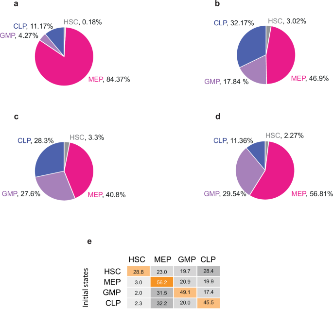
a Normalized basin of attraction size for every cell state at the Boolean model. We derived the basin of attraction using a synchronous updating scheme. The percentage of initial states that lead to a specific cell type is shown, excluding those leading to cyclic attractors. b Relative frequency of cell types observed after a sample of 10⁵ random initial conditions with the continuous model. c Probability distribution as a percentage of steady states reached by stochastic simulation considering a concentration of Oxygen = 0.5 [a. u.]. d Experimentally observed frequencies of hematopoietic lineages^87,94. e Transition matrix showing the probabilities of transitions between all cell types.

Full size image

FOXO3 activity is essential for promoting quiescence in HSCs, with FOXO3 LOF being associated with a loss of quiescence and depletion of the HSCs pool^1,83. In our FOXO3 LOF simulation, we recovered the original 13 fixed-point attractors. However, the HSC basin of attraction is reduced (0.067%, see Supplementary Fig. 55 and Supplementary Table 28). This data is in agreement with the depletion of the HSCs pool observed in vivo. Regarding Mef2c, when the LOF is simulated, the size of the CLP basin of attraction is reduced (6.13%, see Supplementary Fig. 71 and Supplementary Table 36). Even though our model does not recover the expected Mef2c expression in CLP (Fig. 3), the in silico phenotype of Mef2c LOF agrees with experimental data showing impaired lymphopoiesis in vivo in the absence of Mef2c⁸⁴. These results show that the regulatory constraints imposed by Mef2c within the network still influence CLP differentiation, as observed experimentally. In summary, the GOF analysis (Table 2) and the LOF analysis (Table 3) showed a high level of consistency with experimental observations, demonstrating that the model successfully recapitulates the observed phenotypes.

Remarkably, our model allows us to get insights into controversial aspects about the role of some transcriptional factors in the differentiation of HSCs. For instance, it has been reported that HIF-1 is not relevant to maintain the quiescence of HSCs⁸⁵. However, our data show that its absence (Table 3) abrogates the quiescent HSC phenotype. Therefore, our results are consistent with studies that highlight the importance of this transcriptional factor for quiescent HSCs⁸⁶. These data suggest that our model is useful for unraveling controversies about molecular aspects of HSCs differentiation and proposes a dynamic regulatory mechanism that resolves such apparent controversies. Taken together, the mutant simulations and the reproduction of the RNA-seq data demonstrate the effectiveness of our model as a tool to analyze the differentiation of HSCs and show that it constitutes a complex regulatory mechanism underlying this process.

HSC and common progenitors emerge as a result of restrictions imposed by the GRN

Under homeostatic conditions, hematopoiesis is a tightly regulated process where cell populations maintain specific proportions^87,88. Hence, we aimed to understand how hematopoietic progenitor populations emerge within the HSCN. To this end, we initially employed the size of the basins of attraction in the discrete model as an indicator of the magnitude of phenotypic populations (Fig. 5a) under homeostasis and mutant simulations (see Tables 2 and 3).

To evaluate whether the dynamic behavior observed in our model was independent of the mathematical formalism used, it was necessary to transform the Boolean model into ordinary differential equations (ODEs) as described by García-Gómez et al.⁸⁹ After solving the continuous model, we obtained the equilibrium frequencies of each hematopoietic lineage by randomly sampling the state space 10⁵ times. With this approach, approximately 50% of the time our system reached a configuration with intermediate activation values of the nodes (Supplementary Figure 133). However, in the other 50% of cases, our system reached one of the 13 attractors previously identified by the Boolean network. These results indicate that the steady states emerge as a result of restrictions imposed by the GRN and are independent of the mathematical formalism utilized. The observed relative frequencies, without considering the states with intermediate activation values, for HSC, MEP, GMP, and CLP were 3.02%, 46.9%, 17.84%, and 32.17%, respectively (Fig. 5b and Supplementary Tables 45 and 46).

As mentioned before, 50% of the time, our simulations reached states with intermediate values, potentially representing unstable transient states. Therefore, we applied a Kinetic Monte-Carlo algorithm, implemented in the MaBoSS software⁹⁰, to explore the probability space of our asynchronous Boolean network, defined as a continuous-time Markov process. A Markov process is completely defined by a set of transition rates, in this context, derived from the model’s Boolean functions, and a set of probabilistic initial conditions⁹¹.

First, we simulated 10⁶ trajectories, with all initial conditions having the same probability. These trajectories were used to calculate the stationary distribution of the Markov process, which is equivalent to directly calculating the population proportion corresponding to each phenotype^92,93. With this stochastic strategy, we recovered the same set of 13 attractors identified previously by our Boolean and continuous approaches (see Supplementary Table 47). However, we did not identify any additional attractors, emphasizing that the configurations reached by the continuous model with intermediate values are transient configurations. The stochastic simulation recovered frequencies of 40.8% for MEP and 28.3%, 27.6%, and 3.3% for CLP, GMP, and HSC, respectively (Fig. 5c). These probabilities are similar to the relative frequencies obtained by the random sampling of the continuous state space and are closer to the relative frequencies observed in vivo, where MEPs, GMPs and CLPs frequencies are 56.81%, 29.54% and 11.36%, respectively^87,94 (Fig. 5d). However, contrary to what is observed in vivo, in our simulation CLP frequency is greater than GMP. The small discrepancy between the probabilities obtained by the stochastic exploration and the continuous model may emerge as a result of lineage bias of the indeterminate states identified in the continuous exploration under a stochastic framework.

The contribution of HSCs to normal hematopoiesis is a subject of ongoing debate, with evidence suggesting both that HSCs provide a constant supply of blood cells^95,96, and that hematopoiesis is primarily sustained by common progenitors^97,98. Additionally, common progenitors are plastic cell types that, despite having a lineage bias, can give rise to cells of other lineages under certain conditions¹⁵. In this context, the frequency at which common progenitors differentiate is a relevant area of study. Therefore, we computed the transition matrix between all the cell types in our model (Fig. 5e). The transition matrix shows that all cell types have a higher probability of remaining in the same state than differentiating, with HSC having the lowest probability (28.8%), indicating that under our conditions, the HSC state is relatively labile. MEP is the most stable cell type (56.2%); however, their transition to GMP is the most probable, which aligns with their common developmental pathway, as both descend from CMPs⁹⁹. Similarly, GMP is more likely to transition to MEP than to any other cell type. Finally, the transition from common progenitors to HSC is extremely unlikely. In conjunction, these data show that transition probabilities between cell types in our model are in agreement with the differentiation pathways observed in vivo.

Under homeostatic conditions, the frequencies of common progenitors depend on their differentiation and proliferation rates⁸⁸. The differentiation rate, in turn, is influenced by intrinsic factors, such as transcription factors, and extrinsic factors, such as microenvironmental components. Although our model does not incorporate proliferation rates, it allows us to observe that the production of common progenitors is asymmetric and that transitions between common progenitors have a high probability. Collectively, these data suggest that the proportions of each cell type are influenced not only by constraints of the GRN but also by transitions between common progenitors, the microenvironment of the HSCN, and the proliferation rate of each cell type.

HSC differentiation is a stochastic process

Studies on cell fate determination show that this process emerges from complex regulatory networks with deterministic interaction functions in resonance with noise (stochastic resonance)^26,92,93,100. Single-cell transcriptome analyses have revealed the vast transcriptional heterogeneity of HSCs, which increases at the onset of cellular differentiation^101,102. However, the causes and consequences of this heterogeneity remain a topic of debate¹⁸. The available evidence suggests that transcriptional regulation is a stochastic process influenced by random variations in the concentration of transcription factors, which may be due to limited numbers of molecules and also to random thermal fluctuations¹⁰³.

To further investigate the impact of stochastic variation in HSC differentiation, we simulated differentiation trajectories of HSC under different levels of stochastic variation. As mentioned before, our stochastic simulations require a set of transition rates and probabilistic initial states. To introduce stochastic variation in our model, we modified the probability distribution of active and inactive nodes, both independently and combined, at the beginning of the simulation. Each simulation comprised 10⁶ trajectories, all starting from an HSC state but with slightly different initial conditions to mimic a heterogeneous HSCs pool. For each simulation, we tracked the HSC differentiation trajectory and calculated the entropy and transition entropy of the system⁹¹. In the context of a GRN, maximum entropy is observed when all states have equal probabilities. Conversely, when a particular state has a probability of one, the entropy is reduced to zero⁹¹. Transition entropy, on the other hand, measures the disorder at a single trajectory⁹¹. A transition entropy value greater than zero indicates that the system exhibits non-deterministic behavior⁹¹.

When stochastic variation is allowed at inactive nodes (see Fig. 6a), HSC are able to transition to all common progenitor cell types. As expected, HSC frequency is reduced as the level of stochastic noise increases (see Supplementary Fig. 134). At low levels of stochastic fluctuation (p = 0.1), the probability of HSC to transit to GMP is higher than to MEP. However, the opposite occurs when the stochastic fluctuation is higher (p = 0.5). When stochastic fluctuations are permitted at active nodes, HSC differentiates only into CLP and MEP progenitors, but not into GMP (Fig. 6b and Supplementary Fig. 135). The lack of GMP progenitors from this simulation suggests that at least a basal expression of PU.1 is required to reach the GMP cell fate, in agreement with the reported PU.1 dose-dependent function¹⁰⁴. These model results are also in agreement with evidence suggesting that granulopoiesis is disengaged from HSCs differentiation¹⁰⁵. When both active and inactive nodes are allowed to fluctuate stochastically, the HSC state is able to differentiate into the MEP, CLP and GMP progenitors (Fig. 6c). As expected, the level of entropy increases with increased stochastic fluctuations (see Supplementary Figs. 134–136). However, transition entropy is greater than zero only when stochastic fluctuations are allowed in inactive nodes (Fig. 6d–f), indicating that under these conditions, HSC differentiation is stochastic.

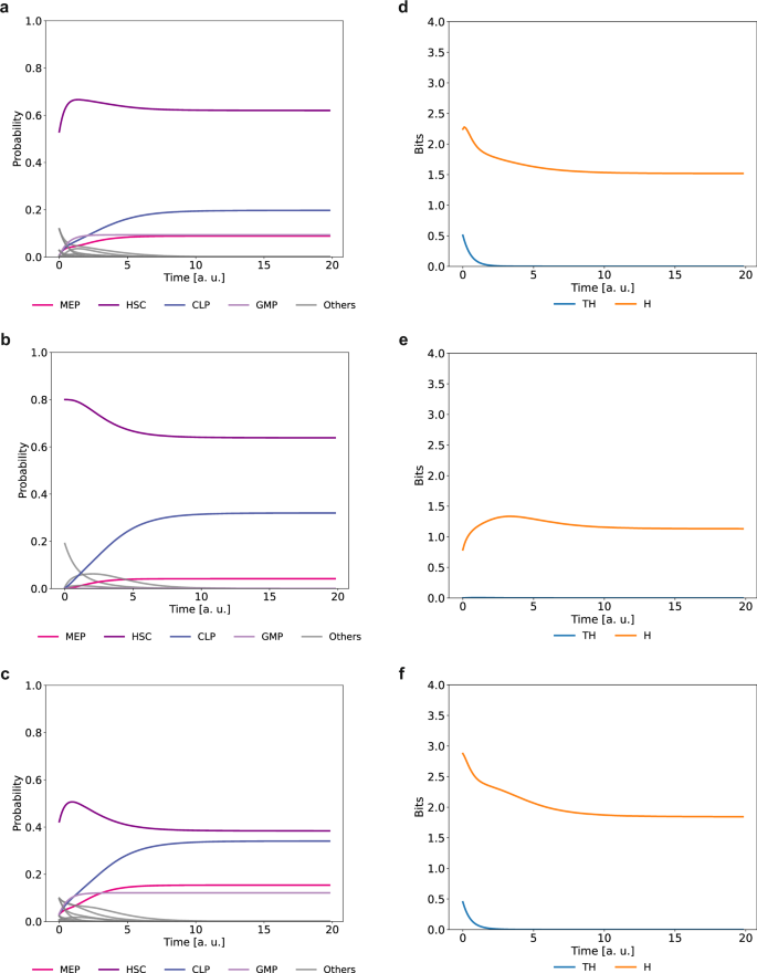
a HSC developmental trajectory when stochastic fluctuations are allowed at inactive nodes in the initial conditions with p([Node = 0]) = 0.8; b when stochastic fluctuations are allowed at active nodes with p([Node = 1]) = 0.8; c when stochastic fluctuations are allowed at both active and inactive nodes simultaneously, using the same probability distributions as in (a) and (b). The lines represent the probability of observing specific cell types over time, while ‘Others’ denotes transient states with mixed lineage markers. Evolution of entropy and transition entropy over time when stochastic fluctuation is allowed at inactive nodes (d), active nodes (e), and both at the same time (f). Here, a. u. means “arbitrary units”.

Full size image

According to the classic model of hematopoiesis, MEPs and GMPs derive from CMPs, however our model did not recover any attractor that can be identified as CMP. Stochastic variation of active and inactive nodes also allows the emergence of transient states characterized by the expression of mixed lineage-markers (identified as “Others” in Fig. 6a–c). Notably, we were able to identify transient states expressing both GATA1 and PU.1, as expected in CMPs⁴³ (see Supplementary Fig. 137). Additionally, we observed transient states expressing mixed lineage cell markers GATA2, PU.1, Meis1, and CEBPA, corresponding to the Multi-Lin* intermediate, previously identified experimentally⁹⁷, and transient states expressing the HSC marker GATA2 along with common progenitor markers GATA1, PU.1., or Gfi1, suggesting an early cell fate lineage restriction. The relevance of these transient states to the final cell fate probability is supported by the fact that those with the highest probability (i.e., GATA2/Gfi1, GATA2/GATA1) precede the most probable transition during HSC differentiation. These data highlight the relevance of heterogeneity within the HSCs pool to achieve proper differentiation.

Oxygen levels influence the differentiation of HSCs

Finally, we focused on evaluating the quantitative effect of variations of input signals, such as oxygen, on the dynamics of the GRN. We used the stochastic model to explore the effect of gradual variations in oxygen levels. Starting at an HSC initial state, we ran stochastic simulations using three different probability distributions of Oxygen as initial states, p[(Oxygen = 1)] = 0, p[(Oxygen = 1)] = 0.5, and p[(Oxygen = 1)] = 1. Since in our network, Oxygen is an input that is not regulated by any other node, once we establish a probability distribution at the beginning of the simulation it remains constant throughout.

When Oxygen concentration was set to 0% (p[(Oxygen = 1)] = 0), we observed an HSC frequency of 28.8% and MEP, GMP, and CLP frequencies of 23%, 19.7%, and 28.4% respectively. (Fig. 5e and Fig. 7a). This mimics the microenvironment found in the HSCN, where low levels of oxygen are necessary to maintain undifferentiated and quiescent HSCs. However, when Oxygen concentration was raised to 50% (p[(Oxygen = 1)] = 0.5), the HSC steady state decreased (Fig. 7b). This decline was further exacerbated when the Oxygen concentration was raised to 100% (p[(Oxygen = 1)] = 1) (Fig. 7c). These data are in agreement with experimental evidence that shows that higher oxygen concentrations are associated with loss of quiescence^5,106,107.

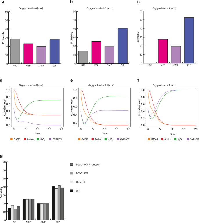
Probability distribution of cell types reached by the stochastic model under different oxygen concentrations. Simulations were initiated from an HSC configuration. Panels show results for a 0% Oxygen, b 50% Oxygen, and c 100% Oxygen. d Average activation value of relevant nodes for ROS homeostasis over time with 0% Oxygen, e 50% Oxygen, and f 100% Oxygen. g Probability distribution of cell types under different stochastic LOF simulations. In this figure, a.u. means ‘arbitrary units’.

Full size image

Interestingly, CLP frequency also increases at higher Oxygen concentrations. It has been shown that high oxygen tension is associated with T cell differentiation¹⁰⁸. However, whether oxygen regulates early lymphopoieses or not remains an open question. Moreover, HSCs and CLPs reside within different bone marrow compartments, HSCs reside in perivascular niches while CLPs are localized at endosteal niches¹⁰⁹. Direct measurements of oxygen tension inside the bone marrow show that endosteal niches exhibit higher oxygen tension than perivascular ones¹¹⁰. Taken together, our results predict a potential link between oxygen tension and early lymphoid differentiation.

Oxygen concentrations impact different aspects of HSC biology, including ROS production and mitochondrial respiration. Thus, to further analyze the effect of oxygen during HSCs differentiation, we examined the behavior of GATA2, H₂O₂, OXPHOS, and Antiox under different Oxygen levels. At 0%, Oxygen, GATA2, and Antiox levels decreased over time while H₂O₂ increased, indicating HSC differentiation into common progenitors. In turn, OXPHOS levels show a transient increase at the beginning of the simulation but then decreased as time passed (Fig. 7d). However, as Oxygen levels increase, OXPHOS levels are sustained (Fig. 7e, f).

Furthermore, we simulated stochastic LOF mutations to analyze how these perturbations affect HSC differentiation. In our Boolean framework, FOXO3 loss of function leads to a reduction in the HSC basin size, suggesting that in the absence of FOXO3, the HSC attractor is less likely to be reached. Similarly, in the stochastic simulation of the HSC developmental trajectory, FOXO3 LOF shows a decrease in the HSC probability (Fig. 7g). Conversely, H₂O₂ depletion has the opposite effect, where HSC probability is increased, indicating a blockage in differentiation. FOXO3 is one of the main regulators of ROS concentration in HSCs, and it has been reported that HSCs lacking FOXO3 show an increase in ROS concentration and a reduced HSC pool. Therefore, we simulated a double FOXO3 LOF/H₂O₂ LOF mutant. In this simulation, the probability of attaining the HSC attractor is midway between those of FOXO3 and H₂O₂ single LOF simulations, indicating that the withdrawal of H₂O₂ can counteract the HSC decrease associated with the absence of FOXO3.

Since the mid-1980s different studies have proposed stochastic models of HSCs differentiation^111,112,113, yet the classical deterministic tree-like model of hematopoiesis remains the dominant perspective, despite the fact this framework is limited to explain several aspects of this process (Fig. 1c). The latter relies on the assumption that stable multi-, oligo-, and bi-potent cell precursors generate two new cell types at every round of differentiation and subsequentially reduce their differentiation potential. Under this model, lineage commitment is obtained by cell-type-specific transcription factors in a deterministic manner. Reconstitution assays, single-cell transcriptomic, and single-cell differentiation analysis have revealed an enormous heterogeneity that not only had been overlooked^{18,88,114,115} but also suggest that HSCs lineage-commitment decision is made at the earliest stages of hematopoiesis, even before cell division occurs¹¹⁶. In consequence, the paradigm of hematopoiesis has been redefined¹⁶ (Fig. 1d), but the underlying dynamic mechanisms of HSCs differentiation still remain to be understood.

Hence, in this work, we pursued a system biology approach to underpin such dynamical mechanisms. To this end, we integrated a large 200-node network grounded on available experimental data on key transcription factors. This network also includes other molecular components, ROS, and their interactions involved in HSC maintenance and differentiation. To pursue further dynamical analyses, this large network was reduced to a 21-node network model which kept the functional feedback loops, thus integrating a set of necessary and sufficient regulatory factors and interactions involved in HSC maintenance and differentiation dynamics (Fig. 2). Such reduced network can be considered a biologically meaningful regulatory core.

We followed a validation protocol to determine whether the developed models were capable of reproducing the cellular behaviors and phenotypes observed experimentally, as summarized in Fig. 8. The first validation of the model involved comparing the attractors attained by the 21-node network with gene expression configurations that have been observed experimentally in HSCs as well as in cell lineages that are derived from such stem cells. We explored the model’s behavior using discrete, continuous, and stochastic frameworks to gain a comprehensive understanding of HSCs development. After validating the models with experimental data (Fig. 4), verifying that the network is capable of reproducing mutant phenotypes observed experimentally (Tables 2 and 3), and explaining apparently controversial observations during HSCs differentiation, we used these models to understand the dynamic mechanisms of HSCN differentiation.

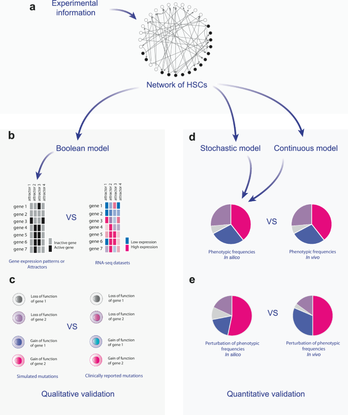
In this work a we used information available in the specialized literature to build a network of interactions present in the differentiation process of HSCs. From this network, three mathematical models were built: a qualitative Boolean model, a quantitative continuous model, and a quantitative stochastic model. b The Boolean model was evaluated by comparing the patterns of genes on and off against RNA-seq data. c In addition, the response of the Boolean model when simulating the loss or gain of function of some genes was compared with experimental data. d On the other hand, the quantitative models were validated by comparing the wild-type frequencies of phenotypes predicted by them against real data obtained through in vivo assays. e Finally, the change in phenotypic frequencies predicted by quantitative models was compared with data obtained from in vivo datasets.

Full size image

The first aspect that we addressed with our network 21-node model or regulatory core was to determine if differentiation is a strictly hierarchical process, excluding plasticity phenomena between common progenitors (Fig. 9a). To explore this assumption, we ran a series of stochastic simulations based on Markov chain approaches and noted that the derived transition probabilities between cell fates qualitatively recover the developmental pathways and temporal patterns observed in vivo. Also, our model recovered plastic dynamic patterns of differentiation rather than a terminal static one (Fig. 9b). While the final size of the common progenitors pool heavily depends on the cell proliferation rate⁸⁸, differentiation probability and cell plasticity are relevant factors during normal hematopoiesis supporting that common progenitors contribute to adult hematopoiesis¹⁰⁵.

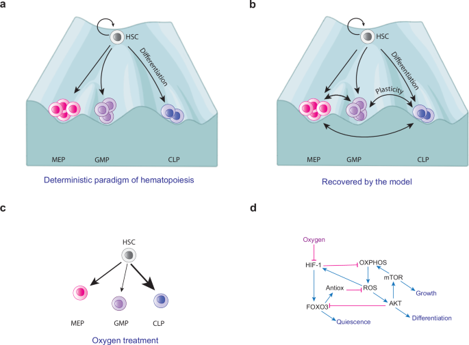
a Deterministic paradigm of hematopoiesis. This conceptual model indicates that hematopoietic lineages do not present plasticity. b In this work we found that hematopoietic progenitors present plasticity among them due to stochasticity. c We found that oxygen exposure increases differentiation rate towards hematopoietic progenitors, which highlights the importance of hypoxia in maintaining physiological conditions within the HSCN. The thickness of the arrows qualitatively represents the frequency of common progenitor cells induced by oxygen treatment. d Molecular mechanism that explains the effect of oxygen on HSCs. This mechanism, derived from our GRN, indicates that oxygen is able to reprogram cell fate decisions through metabolic regulation and ROS production. Blue arrows represent positive interactions; pink lines represent negative interactions. Created with BioRender.com.

Full size image

Single Cell analyses have shown that HSCs comprise a heterogeneous population and that differentiation is preceded by an increased cell-to-cell transcriptional heterogeneity¹⁰². However, the causes and consequences of such heterogeneity are poorly understood. To further investigate the effect of heterogeneity during HSCs differentiation we simulated developmental trajectories of a heterogeneous HSCs pool. We found that stochastic fluctuations of the inactive nodes at the expression configuration that corresponds to the HSC state are necessary to recover all common progenitors, indicating that cell fate determination results from a stochastic process (Fig. 6b, d).

Interestingly, our model predicts that HSC will differentiate at a higher proportion into MEP and CLP than into GMP (Fig. 6b, c). There is evidence suggesting that granulopoiesis is disengaged from HSCs differentiation and that hematopoiesis is sustained mainly by common progenitors^98,105, in line with the results obtained by our model where GMPs differentiated at a lower proportion. While the cellular contribution of HSCs and common progenitors during hematopoiesis under homeostatic conditions is still a matter of debate⁹⁵, our model recapitulates experimental evidence and provides a dynamic mechanism to explain the importance of transcriptional heterogeneity in HSCs differentiation.

Next, we addressed the effect of the microenvironment on hematopoiesis. To this end, we simulated the effect of varying oxygen availability in the HSCN. We found that oxygen was capable of increasing the differentiation speed of hematopoietic precursors while reducing the pool of HSCs (Fig. 7). In this sense, the results indicate that the presence of oxygen in the HSCN is sufficient to promote HSCs differentiation (Fig. 9c). To further identify the molecular cause underlying this phenomenon, we analyzed which regulatory motifs within the GRN (Fig. 2) explain the role of oxygen on HSCN differentiation (Fig. 9d). Naturally, H₂O₂ activates growth and differentiation by stimulating AKT, which in turn triggers the activation of differentiation circuits in HSCs. However, the hypoxic context inhibits these indirect functions of ROS (Fig. 9d). On the other hand, the presence of oxygen abrogates this inhibition mechanism, allowing ROS to increase through the action of OXPHOS (Fig. 9d). Contrary to what was thought about ROS, at controlled levels, they participate as a second messenger to control HSCs differentiation.

Furthermore, our results also suggest the existence of an alternative mechanism that reduces HSC quiescence and links transcriptional heterogeneity and metabolism. To be precise, we observed that the frequency of the HSC phenotype is reduced by increasing transcriptional noise (Supplementary Fig. 134), which also occurs by increasing the oxygen availability in the HSCN (Fig. 7a–c). Consequently, it is possible that the augment in oxygen availability triggers transcriptional fluctuations as a side effect. We think that such a mechanism is feasible since it has been reported that in oxygen-exposed bacterial cultures, the transcription is highly heterogeneous compared to anaerobic cultures¹¹⁷. Perhaps hypoxia is a control factor to keep the plasticity of HSC differentiation limited, in order to provide physiological stability to the production of the different lineages derived from these cells. Collectively, these mechanisms open the door to the possibility that metabolic modifications could serve to control the hematopoietic processes of cellular differentiation and plasticity, as some have recently suggested¹¹⁸.

In conclusion, in this work, we used a system biology theoretical and integrative approach by proposing a set of mathematical and computational models to study HSCs proliferation and differentiation in the HSCN. We found that hematopoiesis is a plastic process that is strongly influenced by external factors including the bioavailability of growth signals such as cytokines and oxygen within the HSCN microenvironment. Hence, we provide here a model of a dynamic complex network of 21 nodes as a key regulatory mechanism involved in HSCs dynamics and the physiological importance of maintaining the HSCN under hypoxia. Our results also suggest that the observed patterns of HSC maintenance and differentiation result from a stochastic resonance process that involves deterministic network interactions coupled with random fluctuations.

Construction of the network

We performed a manual search in the literature and databases Harmonizome 3.0¹¹⁹ and Kyoto Encyclopedia of Genes and Genomes (KEGG)¹²⁰ to identify key molecules in the regulation of metabolic and differentiation processes of HSCs. As a result of this search, it was possible to build a GRN of interactions between 200 main biological components that regulate the differentiation of HSCs (Supplementary Data 1). The complexity of Boolean networks increases exponentially as the node number rises, making the dynamical analysis of large networks computationally unfeasible. However, research has demonstrated that within such large biological networks, it is possible to identify smaller regulatory cores that are both modular and robust, and still comprise the functional regulatory feedback loops that are responsible for the network´s stable states or attractors^36,37,77. These properties allow the reduction of large networks into smaller ones that recover the attractors and dynamic behavior of the original network by collapsing its linear pathways. To this end, we used the GINSIM³⁵ software to reduce the 200-node network to a regulatory core of 21 nodes.

Boolean modeling of the network

After obtaining the reduced interaction network, we searched for biological information to apply Boolean formalisms to model it. In this sense, Boolean networks are composed of nodes that, in the context of biological GRNs, represent regulatory molecules such as transcription factors, metabolites, or signaling molecules. Every node can be associated with only two discrete states, either 0 or 1, depending on its functional activity. When a node is active, it has a value of 1; otherwise, it has a value of 0. The state of a node at a specific time step depends upon the activation state of its regulators in the previous time step. This value is expressed by a Boolean function, also called a logical rule, which is expressed with the logic operators AND, OR, and NOT, these logical rules take the general form:

where x_i(t+1) represents the state of node x_i at time t+1, and x₁(t),…,x_k(t) represents the activity states of its regulators at time t. A Boolean function was defined for each node based on experimental data. When no post-transcriptional regulation data is available, a transcription factor is considered active if its expression is detectable. For ROS molecules, which often exhibit a graded distribution, we considered their lowest concentration as 0 and the highest concentration as 1. Enzymes and signaling molecules are considered active when they exert their catalytic function.

The corresponding Boolean functions of the reduced network, known as the GRN of HSCs, are shown in Table 1. The experimental evidence supporting the logic rules is provided in Supplementary Note 1. We used both synchronous and asynchronous updating schemes to exhaustively explore all possible initial states of the system. From each initial state, we iteratively applied the logical rules until the system reached a stable activity configuration, known as a steady state or attractor. In molecular networks, attractors are associated with gene expression configurations that characterize specific cell states or phenotypes^57,58,121. Simulations using the synchronous updating scheme frequently result in the recovery of multiple cyclic attractors, which are not observed when employing the asynchronous updating scheme^89,122,123. Unlike the synchronous updating scheme, asynchronous updating more closely resembles biological processes that occur at different time steps¹²⁴, such as transcriptional regulation, phosphorylation, or redox reactions^125,126,127. Fixed-point attractors are generally understood as stationary robust phenotypes, whereas cyclic attractors are interpreted as recurring patterns of molecular activation^57,58. Therefore, for further analysis, only fixed-point attractors were used. A full set of attractors recovered by synchronous and asynchronous schemes is provided in Supplementary Information and Fig. 3, respectively. These analyses were conducted with the R package BoolNet¹²⁸.

Selection of genetic markers

To identify and interpret the results obtained through Boolean modeling of the GRN, four genetic markers were selected to identify the differentiation fates that HSCs might present. To label the attractors corresponding to HSCs, GATA2 was selected as a marker, because its importance in the functioning of these cells has been demonstrated⁶⁴. To identify the attractors that correspond to MEPs, GATA1 was selected as a molecular marker since this gene actively participates in maintaining the main functions of this cell type⁶¹. On the other hand, to identify GMPs, the PU.1 marker was selected, since it has been shown that its expression is essential to regulate the functions of this cell type⁶². Finally, to identify the attractors that correspond to CLPs, the marker Gfi1 was selected since it has been seen that this gene actively participates in the specific regulation of this phenotype⁶³. Therefore, in this work, HSCs are identified as GATA2⁺ cells, MEPs as GATA1⁺ cells, GMPs as PU.1⁺ cells, and CLPs as Gfi1⁺ cells.

Validation protocol for Boolean modeling

For the perturbation analysis, we simulated 10³ random networks of the same size as the HSC regulatory network. For structural perturbations, we randomly modified the Boolean functions of each random network one hundred times. We then recorded the percentage of original attractors recovered and compared this with the performance of the HSC regulatory network. For dynamic perturbations, we generated a separate set of 10³ random networks. In each network, we randomly selected 10³ states, induced random bit flips, and measured the Hamming distance between the successor states of the perturbed and unperturbed networks.

To further validate the Boolean model of the GRN, a series of gain-of-function (GOF) and loss-of-function (LOF) experiments were performed to simulate the emergence of mutations in the overall network structure. We implemented these simulations by setting the value of the mutated node to 0 for LOFs or 1 for GOFs with the R package BoolNet¹²⁸. Mutant simulations were conducted using both synchronous and asynchronous updating schemes (see Supplementary Information). Next, the effect of each mutation on the attractors landscape, measured as changes in the basin of attraction of each cell type, was analyzed and compared with available information to determine whether the model could reproduce the reported findings (Table 2 and Table 3). The basin of attraction is defined as the set of initial conditions in the state space that converge to the same steady state. It can be computed under a synchronous updating scheme, where any initial state can be assigned to a particular stable state.

Additionally, the gene expression patterns corresponding to the wild-type network and its differentiation fates were compared with data obtained from RNA-seq, in order to test the existence of the behaviors predicted by the model in nature.

Processing RNA-seq datasets

To compare the expression patterns predicted by the Boolean model with data obtained from RNA-seq, we first searched GEO (Gene Expression Omnibus) for RNA-seq data corresponding to the phenotypes studied by the GRN. In this case, we used purified and publicly available data of HSCs, MEPs and GMPs. Concerning to these databanks, the dataset of HSCs was obtained by Bloom et al.⁶⁷(accession number: GSE213596); The MEPs dataset was obtained by Lu et al. ⁶⁸ (accession number: GSE112692), and the GMPs’ dataset was obtained by Yáñez et al.⁶⁹ (accession number: GSE88982). Next, we normalized these data using the Transcripts Per Million (TPM) convention¹²⁹. We repeated this procedure for the housekeeping genes GAPDH, TBP, CYC1, and HPRT¹³⁰, and we compared the values of the genes belonging to the GRN against the RNA-seq datasets. If the value of each gene was lower than the expression value of the normalized housekeeping genes, then a value of zero was assigned to the gene evaluated. Otherwise, the value of one was assigned to the evaluated gene.

Continuous modeling of the network

To extend our Boolean model into a continuum formalism, we translated the discrete Boolean functions into continuous form using Zadeh’s fuzzy logic operators as previously implemented^89,131,132. For example, the Boolean expression A AND B is true when both A and B are true. This expression is replaced by the fuzzy logic operator min(A,B). The idea behind this translation is that in a continuous system, the truth value of A AND B is as small as the lesser of the two individual truths. Following this logic, A OR B is replaced by max(A,B), and the Boolean expression NOT A is replaced by 1-A. Consequently, in the continuous model, the state of each node is described by the following ordinary differential equation:

The first part of the equation is a sigmoid function that describes the production rate of x_i. The parameter h determines the strength of the interaction and controls the shape of the sigmoid function. For values around 100, the curve approximates a step function, while for values around 50, the shape resembles a logistic curve. w represents the logical function in continuous form, translated with fuzzy logic operators. The second part of the equation is a linear term representing the decay rate of x_i with the parameter γ. We obtained the frequency of each stable state by sampling the state space from 10⁵ random initial conditions (see Supplementary Information). This analysis was implemented in R.

Stochastic exploration of the network

To analyze differentiation probabilities between steady states, we simulated 10⁶ stochastic trajectories using a Kinetic Monte-Carlo algorithm applied to the asynchronous Boolean dynamics, following the protocol reported by Stoll et al.⁹¹. This algorithm associates a transition rate to each node, based on Boolean logic rules, and given a set of probabilistic initial conditions, produces stochastic trajectories used to compute transition probabilities. The probability of the system being in a state S at a discrete time τ is given by the following equation:

where Δt is the length of a continuous time interval, and P[s(t) = S] represents the probability of the system being at a state S at any time t within this interval. Instantaneous probabilities converge to a stationary distribution after a certain amount of time. From the stationary distribution, the probability of a specific cell type can be computed by clustering the individual probabilities of states that have non-zero values in the selected markers (see Supplementary Information).

Entropy, H, represents the disorder within the system. In this context, a system where all states have equal probability has maximum entropy. Conversely, a system where a single state has a probability of one has zero entropy. Entropy can be calculated with the following equation:

where P[s(τ)=S] is the probability of the system being in state S at time τ. In contrast to entropy, which measures the whole system’s disorder, transition entropy (TH) measures a single trajectory. Given a state S, there is a set of transitions (S,to S^{prime}) with a probability ({PS}to S^{prime}). The following equation allows to compute TH for each state:

Transition entropy allows us to assess how deterministic the system’s dynamic is; a system that can only make a single transition has zero transition entropy. In conjunction, entropy and transition entropy provide a global characterization of the system’s dynamics. Stochastic explorations, entropy, and transition entropy calculations were performed with the MaBoSS software⁹⁰.