A unified deep framework for peptide–major histocompatibility complex–T cell receptor binding prediction

Antigenic peptides presented by the major histocompatibility complex (MHC) can induce immune responses by being recognized by T cell receptors (TCRs), which carry the CD8 antigen on the surface of T cells¹. Investigating the binding mechanisms among peptides, MHCs and TCRs is of great importance for cancer immunology, autoimmunity antigen discovery and vaccine design². However, due to the intrinsic complexity of such binding mechanisms, the experimental detection and determination of the binding among peptides, MHCs and TCRs are time-consuming and expensive³. To solve these problems, computational methods have been developed in recent years.

In peptide–MHC–TCR (P–M–T) binding, the interaction between the peptide and MHC plays an important role. There are two main computational methods for the prediction of peptide–MHC (P–M) binding: scoring-based methods and learning-based methods. Scoring-based methods utilize multiple statistical scoring functions to calculate the binding probability of the input sequences^4,5. Learning-based methods learn representations for input sequences via deep neural networks such as attention networks, long short-term memory networks and transformers to model interactions between peptides and MHCs^{6,7,8,9,10,11,12}. To achieve effective peptide–TCR (P–T) binding prediction, computational tools such as TEIM³, TCR-AI¹³ and PanPep¹⁴ have been proposed. These methods apply machine learning techniques to predict the interaction between a CDR3 sequence (one of the core binding regions) and a peptide sequence. Instead of predicting the pairwise binding possibility, such as P–M and P–T, there are works that take the peptide, MHC and TCR sequences as the input, and directly predict the binding possibility of P–M–T. For example, pMTnet¹⁵ uses the transfer learning technique to train a model, which can predict the TCR binding specificity of peptides presented by a specific class I MHC.

With the accumulation of data and the development of the aforementioned deep learning techniques, the predictive performance of P–M–T, P–M and P–T has improved. However, in cancer immunotherapy and other related immune therapies, there is still an urgent need to further improve the binding prediction accuracy, especially for the P–M–T binding prediction. Existing approaches typically focus on only one of the three interaction types (P–M–T, P–M or P–T), resulting in the incomplete utilization of available multifaceted binding information. For example, in P–T binding prediction, the P–M binding information is usually neglected. We claim that the binding mechanisms among peptides, MHCs and TCRs are mutually related, and the accurate binding prediction of P–M–T, P–M and P–T may boost the overall performance. Simultaneously, effective learning of these three tasks can mitigate, to some extent, the scarcity of existing datasets, which is a notable challenge in this field.

In this work, we introduce UniPMT, a unique unified multitask learning model using heterogeneous graph neural networks (GNNs) for predicting the TCR binding specificity of pathogenic peptides presented by class I MHCs. Our model provides an example of unification on three critical levels. First, at the data level, we collect a unified dataset that enables the integration of diverse nodes (P, M and T) and edge types (P–M–T, P–M and P–T), thereby reflecting a comprehensive manner for synthesis. Second, at the framework level, UniPMT uses a heterogeneous GNN, providing a unified and cohesive structure that effectively captures the intricate interactions among peptides, MHCs and TCRs. This framework underscores our integrated approach to model complex biological interactions. Finally, at the training level, UniPMT adopts a multitask training strategy, utilizing both deep matrix factorization (DMF)¹⁶ and contrastive learning¹⁷ to facilitate a cross-featured learning process. This tripartite approach to unification in UniPMT not only highlights the versatility and sophistication of our model but also sets a precedent in the realm of immunological prediction models.

We systematically validate the performance of UniPMT using P–M–T, P–M and P–T validation datasets and demonstrate its advances over previous works. The proposed UniPMT consistently achieves state-of-the-art performance in P–M–T, P–M and P–T binding prediction tasks, where the promising improvement on P–M–T is 15% in area under the precision–recall curve (PR-AUC). At the same time, we demonstrate its feasibility in clinical applications, such as the prediction of neoantigen-specific TCR binding, T cell cloning and prediction of potential P–M–T binding triplets. These applications, especially potential P–M–T binding triplet prediction, have an irreplaceable role in special clinical immunotherapy application scenarios, such as TCR-gene-engineered T cells, in situations where tumour-infiltrating lymphocytes are difficult to sort. In general, UniPMT focuses on the long-standing problem of P–M–T binding prediction, revealing biological insights on antigen presentation and immune stimulation, which can serve as a basis for constructing biomarkers to predict the immunotherapeutic response.

UniPMT overview

UniPMT is a multitask learning framework using GNNs to predict the TCR binding specificity of pathogenic peptides presented by class I MHCs. UniPMT innovatively integrates three key biological relationships—P–M–T, P–M and P–T—into a cohesive framework, utilizing the synergistic potential of these relationships¹⁸. As shown in Fig. 1, UniPMT comprises a structured approach beginning with graph construction, where biological entities (evolutionary scale modeling (ESM)¹⁹ is applied to learn the initial embedding of P and T, and the TEIM method is applied to obtain the pseudo-sequence of M) are represented as nodes and their interactions are represented as edges. This is followed by graph learning via GraphSAGE²⁰, which learns robust node embeddings. Finally, UniPMT uses a DMF-based learning framework¹⁶ to unify binding prediction tasks for P–M–T, P–M and P–T interactions, harnessing a comprehensive and integrated learning strategy. Following differential training, the prediction output was generated comparatively. UniPMT outputs a scalar value as the binding probability between 0 and 1, where higher scores represent higher binding probabilities. Unlike existing works that focus only on one binding prediction task, our proposed UniPMT performs the P–M–T, P–M and P–T binding prediction tasks in a unified manner. With the multitask learning strategy and the elaborately designed model structure, UniPMT achieves state-of-the-art performance on all three binding prediction tasks.

The P–M–T, P–M and P–T relationships are first represented as a graph, where the initial embedding of P and T is learned via ESM¹⁹, and that of M is its pseudo-sequence³. Then, a GNN is applied to learn the embeddings of each input node. Finally, a DMF-based learning strategy is applied to unify the binding prediction tasks for P–M–T, P–M and P–T. w and y denote the weights and prediction scores, respectively.

Full size image

Performance on P–M–T binding prediction

In this section, we investigate the performance of UniPMT on P–M–T binding prediction on the dataset in pMTnet, including 29,342 positive training pairs and 551 positive testing pairs (we keep those pairs with class I MHC pseudo-sequence available). More details of the dataset and data splitting are summarized in the ‘Data processing’ section. We compare our proposed method with pMTnet, TEIM and PanPep, where TEIM and PanPep are retrained on the dataset. We summarize the results of UniPMT and the baselines in Fig. 2a,b, where the results of pMTnet are derived from the predictions of the original work¹⁵. In general, UniPMT achieves an average of 96% in the area under the receiver operating characteristic curve (ROC-AUC) and 72% in PR-AUC, which outperforms baselines by at least 4% in ROC-AUC and 15% in PR-AUC. Achieving this improvement is possible because our multitask learning strategy—as the P–M–T binding prediction task—relies on all three types of binding information.

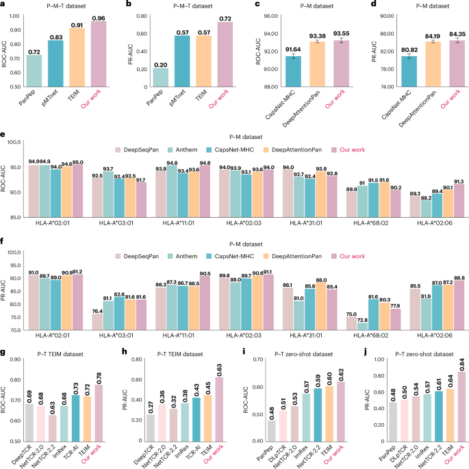
a,b, ROC-AUC (a) and PR-AUC (b) of UniPMT and the baselines on the P–M–T dataset. c,d, ROC-AUC (c) and PR-AUC (d) of UniPMT and the baselines on the P–M dataset (shown as mean values ± s.d.). e,f, ROC-AUC (e) and PR-AUC (f) of UniPMT and the baselines on the P–M dataset and among the seven alleles with more than 1,000 pairs in the testing set. g,h, ROC-AUC (g) and PR-AUC (h) of UniPMT and the baselines on the P–T TEIM dataset. i,j, ROC-AUC (i) and PR-AUC (j) of UniPMT and the baselines on the P–T zero-shot dataset.

Source data

Full size image

We further compare our UniPMT with pMTnet, TEIM and PanPep on the neoantigen P–M–T testing set, which is generated from the original P–M–T testing set by restricting the negative T to known neoantigen-specific Ts and not shuffling P–M in negative sampling. The P–M–T training set remains the same. More details of the dataset and data splitting are summarized in the ‘Data processing’ section. We present the results of UniPMT and the baselines in Table 1. In general, UniPMT achieves 72.14% in ROC-AUC and 28.36% in PR-AUC, which outperforms all baselines by at least 8.86% in ROC-AUC and 5.58% in PR-AUC. We observe that the performance on the neoantigen dataset is lower than the previously reported P–M–T binding prediction results, which is consistent across all baselines. This can be attributed to two main reasons. (1) Fixing P–M and shuffling T increases the difficulty of prediction by removing the influence of easier P–M binding patterns. (2) The neoantigen dataset is relatively small, which might result in weaker learning of this specific subset during model training.

Performance on P–M binding prediction

In this section, we investigate the performance of UniPMT on P–M binding prediction. We compare UniPMT with CapsNet-MHC⁷, DeepAttentionPan¹⁰, Anthem⁴ and DeepSeqPan²¹ on the Immune Epitope Database (IEDB) dataset (MHC class I binding prediction)²², where Anthem and DeepSeqPan can only be evaluated on a specific allele. We keep those pairs with class I MHC pseudo-sequence available, resulting in 156,844 pairs. We randomly split the dataset into five folds and take one of the five folds for testing and the remaining four folds for training. More details on the dataset and data splitting are demonstrated in the ‘Data processing’ section. We show the averaged results of UniPMT and the baselines in Fig. 2c,f. UniPMT achieves 93.55% (s.d., 0.27) in ROC-AUC and 84.35% (s.d., 0.79) in PR-AUC, DeepAttentionPan achieves 93.38% (s.d., 0.17%) in ROC-AUC and 84.19% (s.d., 0.52%) in PR-AUC and CapsNet-MHC achieves 92.85% (s.d., 0.32%) in ROC-AUC and 83.21% (s.d., 0.57%) in PR-AUC. In general, UniPMT outperforms state-of-the-art baselines by at least 0.17% in ROC-AUC and 0.16% in PR-AUC. We further take the seven alleles with more than 1,000 pairs in the test dataset for analysis (taking one of the five folds as an example), and UniPMT achieves the best performance on four out of the seven alleles in both ROC-AUC and PR-AUC. The results demonstrate that our proposed model achieves promising results in the P–M binding prediction task.

Performance on P–T binding prediction

In this section, we investigate the performance of UniPMT in P–T binding prediction. We investigate UniPMT under two settings: the general setting and the zero-shot setting. All baselines are retrained on our datasets.

For the general setting, we use the dataset in TEIM, which contains a total of 19,692 positive P–T pairs. Unlike TEIM, we randomly split the dataset into five folds, where a P in one fold also occurs in the remaining four folds in general. We follow the same strategy for five times more negative P–T pair generation and validation as that of TEIM. The baselines we compare include NetTCR 2.2 (ref. ²³), TEIM, TCR-AI, ImRex²⁴, NetTCR 2.0 (ref. ²⁵) and DeepTCR²⁶. We summarize the results of UniPMT and the baselines in Fig. 2g,h. In general, UniPMT achieves an average of 78% in ROC-AUC and 63% in PR-AUC, which outperforms the baselines by at least 5% in ROC-AUC and 18% in PR-AUC. In addition to the privilege of our proposed model design, we owe this promising result to the P–M and P–M–T information that UniPMT further captured, which implicitly boosts the learning of P–T binding prediction.

For the zero-shot setting, we use the dataset in PanPep, which contains a total of 32,080 positive P–T pairs, including 31,223 pairs in the training set and 857 pairs in the testing set. Unlike PanPep, we generated the same number of negative P–T pairs via random shuffling instead of using a control set. More details of the dataset and data splitting are summarized in the ‘Data processing’ section. We compare our proposed method with NetTCR 2.2, TEIM, ImRex, NetTCR 2.0, DLpTCR and PanPep. We present the results of UniPMT with the baselines in Fig. 2i,j. In general, UniPMT achieves an average of 62% in ROC-AUC and 84% in PR-AUC, which outperforms the baselines by at least 2% in ROC-AUC and 20% in PR-AUC.

Ablation study

To demonstrate the superiority of our multitask learning strategy, we generate three variants of our UniPMT named P–M–T only, P–M only and P–T only. P–M–T only denotes that we only consider the P–M–T edges when generating the input graph and only learn the P–M–T binding prediction task. The other two variants are similarly defined. We evaluate all three variants together with our UniPMT on the P–M–T dataset, P–M dataset and P–T zero-shot dataset. The results of UniPMT and its three variants are summarized in Table 2. We observe the following. (1) For the P–M–T binding prediction, all three types of edge provide valuable information for the target task. P–M–T and P–T information show greater importance than the P–M information, which aligns with the biological understanding that the P–T and the overall P–M–T interactions are more directly relevant to the final binding outcome. P–T edges are valued most for the P–M–T binding prediction task. This may be because the P–T learning in UniPMT is derived from P–M–T learning, which considers all M possibilities and captures more generalized P–M–T binding patterns. In addition, the P–T dataset is labelled (both positive and negative samples), providing more accurate binding signals. (2) For the P–M binding prediction, P–M edges are valued the most, and the P–M-only variant even achieves on-par performance with the full model. This is because the P–M binding prediction in UniPMT is taken as a sub-step for the P–M–T and P–T predictions, making the P–M edges offer a positive influence on both P–M–T and P–T predictions. However, there is no direct inverse influence from the P–M–T and P–T edges to the P–M binding prediction. This conforms to the results in the ‘Performance on P–M binding prediction’ section, where our proposed UniPMT achieves limited improvements compared with models based on learning P–M information only. The P–M–T-only and P–T-only variants achieve similar results, which may be because they contain a similar amount of valuable information (either direct P–M binding information from P–M–T edges or hidden P–M information from P–T edges) for P–M binding prediction. (3) For the zero-shot P–T binding prediction, the P–T pairs in the training and testing sets are mutually exclusive. This is why the P–T-only variant achieves inferior results. The P–M-only and P–M–T-only variants involve the labelled P–M edges that may contain hidden information relating to the P–T binding prediction in the testing set, thereby achieving better performance.

Clinical applications of P–M–T binding prediction

Adoptive cell transfer shows great potential as a cancer immunotherapy approach, whereas its effect largely relies on the selective expansion of tumour-specific T cells within the graft^27,28. The critical factor in optimizing adoptive-cell-transfer-based immunotherapy is the precise identification of T cells that recognize and respond to specific neoantigens^29,30. We collected 312 P–M–T binding triplets from our base dataset, where the neoantigens, their presenting MHCs and binding TCRs were experimentally validated. Following the ‘Performance on P–M–T binding prediction’ section, ten times more negative triplets were generated by random shuffling. We test whether the immune-responsive T cells were correctly identified by UniPMT and compare its results with PanPep, pMTnet and TEIM. As shown in Fig. 3a,b, our UniPMT achieves the best performance with ROC-AUC of 94.29% and PR-AUC of 72.15% for immune-responsive T cell identification of neoantigens, which is 2.91% and 17.62% better than the previous best results, respectively. These results demonstrate the superiority of our model in yielding important implications for both cancer vaccines and associated immunotherapies.

a,b, ROC-AUC (a) and PR-AUC (b) of UniPMT on a clinical dataset of neoantigen-specific TCRs. c,d, Correlations between the clonal ratio of T cells and our predicted binding score (c) and the UMI count (d) in the log–log scale.

Source data

Full size image

Indicative result on clonal expansion of T cells

As TCRs exhibiting higher binding affinities are more likely to undergo clonal expansion, the predicted binding scores by UniPMT may indicate the expansion ratio of T cells. To demonstrate the indicative role of our model in the diverse expansion of global T cell clones, we analyse a single-cell dataset derived from a healthy donor without any known viral infection, containing profiles of CD8 antigen T cells that are specific for 44 distinct P–M complexes³¹. For each T cell in this dataset, we predict its binding score to the 44 P–M complexes and compute the Spearman correlation coefficient with the clonal expansion ratio. The same correlation analysis is also performed using the original unique molecular identifier (UMI) count. As illustrated in Fig. 3c,d, the predicted binding scores show a positive correlation with the clonal expansion ratio of T cells (with a correlation score of 0.2553). By contrast, the correlation between UMI count and clonal expansion is considerably weaker (with a correlation score of –0.07), suggesting that the UMI-based indicator is not suitable for qualitatively reflecting the clonal expansion of T cells. These results suggest that UniPMT can be a clonally expanded indicator in a qualitative manner to a certain extent.

Crucial sites analysis in P–M–T binding

To show the interpretability of our embedding learning module, we predict the key binding sites of CDR3 β and the peptide in P–M–T binding according to the importance of each amino acid. The importance of each amino acid is computed by the difference between the initial sequence embedding and the sequence embedding after alanine substitution^32,33 (replaces an amino acid with alanine (A) and examines the variant’s binding energy between P–M and TCR β by structural simulation). We take 1QRN and 2PYE as two examples, and summarize the binding energy distribution before and after the alanine substitution of 1QRN in Fig. 4a. The ‘base’ denotes the binding energy of the original model of 1QRN based on its three-dimensional (3D) complex structure. R3, L6 and Q13 are the predicted key sites, and R3A, L6A and Q13A denote their corresponding binding energy distribution after alanine substitution. G9 is a randomly selected site from the remaining sites, and G9A denotes its corresponding binding energy distribution after alanine substitution. As shown in Fig. 4a, variants on the predicted key binding sites show a much higher binding energy difference to the base than that of the predicted unimportant binding sites.

a, Structure-based crucial site evaluation on 1QRN. b, Enlarged views before and after alanine substitution on 1QRN. c, Correlation between the 15 predicted P–M–T triplet ranks and their binding energy. d–f, Detailed structure-based binding energy of 3 out of the 15 selected triplets in Fig. 4c at different intervals: 1–10 (2nd) (d), 10–100 (81st) (e) and 100–1,000 (597th) (f). Elect., electrostatic energy; vdW, van der Waals energy.

Source data

Full size image

In addition to the binding energy analysis, we also analyse the distance between the atomic hydrogen bonds and α carbon atoms in the detailed structural diagram. As shown in Fig. 4b(i), we examine the hydrogen bond and α carbon atom distance between the peptide and CDR3 β before and after the alanine substitution on 1QRN. The enlarged view in Fig. 4b(ii) shows the interactions of R95, L98, Q106 and G101 (corresponding to sites R3, L6, Q13 and G9, respectively) with the peptide before alanine substitution. Figure 4b(iii) shows the interactions of position R95 (R95A), L98 (L98A), Q106 (Q106A) and G9 (G9A) with the peptide after alanine substitution. Taking R95A as an example, we find that the closest hydrogen-bond distance between TCR-R95 and peptide-Y5 changed from 2.1 to 5.0. For L98A, the distance between the α carbon atom of TCR-L98 and the peptide-Y8 shows a slight change from 6.5 to 6.4. However, the interaction distance between the hydrogen atoms becomes much larger (from 2.0, 3.6 and 4.2 to 3.0, 4.6 and 4.4, respectively), which may lead to better binding. As a control, the distance between the α carbon atoms is slightly reduced (from 5.6 to 5.4) for G9A, and the interaction distance changes between the hydrogen atoms before and after substitution is also relatively small (from 3.9, 4.6 and 4.6 to 2.3, 3.2 and 3.1, respectively), leading to a slight change in binding energy (from –62.5582 to –65.3066). The above analysis showcases the critical role of our embedding learning module in the prediction of key sites in P–M–T binding. Similar results can be witnessed on 2PYE (Supplementary Section 1).

P–M–T binding discovery

In T cell therapy, the P–M–T binding prediction is especially important for tumour-infiltrating lymphocytes that are not well enriched and cannot be screened for antigen-specificity binding experiments. In this section, we evaluate the ability of our model on potential P–M–T binding triplet prediction. For the validated neoantigen dataset in the Cancer Antigens Database³⁴, we selected neoantigen peptides that intersected with our dataset and obtained a total of 43 peptides. We enumerate all possible P–M–T triplets according to the MHCs and TCRs in our collected base dataset. For all possible P–M–T triplets, we predict their corresponding P–M–T, P–M and P–T binding scores, and keep those with valid predicted scores (larger than 0.5) on P–M–T, P–M and P–T binding only, resulting in 139,348 potential pairs ranked according to their predicted P–M–T binding scores. We take the predicted peptide and the potential CDR3 as the model and calculate the binding energy between the peptide-HLA and TCR β to check whether the binding energy is positively correlated with the predicted P–M–T score. For an accurate energy calculation, we select 15 sequences that are similar to the template molecules in the Protein Data Bank library for modelling and performing energy optimization comparisons. As shown in Fig. 4c, the correlation between the rank of the 15 selected sequences and their structure-based binding energy is 0.796, demonstrating that our predicted binding score can serve as a good indicator for estimating the binding energy of P–M–T triplets. Figure 4d–f shows the detailed binding information of three examples from different ranking intervals out of the 15 selected sequences.

Owing to the broad clinical applications of recognizing the TCR binding specificity of pathogenic peptides presented by class I MHCs, there is an urgent need for effective P–M–T binding prediction. We propose UniPMT, a universal framework for a robust P–M–T binding prediction model for various settings, including P–M–T, P–M and P–T binding predictions. The advantage of UniPMT lies in its holistic approach, integrating distinct datasets and learning tasks within a single model. This integration allows for a comprehensive understanding and prediction of the binding phenomena, enhancing the applicability of the model in immunotherapy prediction, and revealing deep biological insights.

Although UniPMT outperformed other methods in the prediction of P–M–T, P–M and P–T binding predictions, several aspects can be further improved. (1) UniPMT relies on heterogeneous GNN training, where the performance can be further improved when more training data are available. (2) UniPMT considers the interaction of the CDR3 β chain of TCR with the peptide only, which is the same as most of the previous studies^14,15. However, catch bonds in other chains may also play an important role in the TCR prediction of neoantigens. Therefore, considering more information, such as the α chain, is expected to further improve the model’s performance. (3) With the increasing 3D crystal structure data, further embedding the 3D data of peptides, MHCs and TCRs may also help with the P–M–T binding prediction.

Data processing

Base dataset processing: we collect a base dataset, in which the P–M binding dataset is obtained from BigMHC³⁵; the P–T binding dataset is obtained from PanPep, DLpTCR³⁶ and NetTCR³⁷; and the P–M–T binding dataset is obtained from ERGO³⁸ and pMTnet. To further expand the number of P–T pairs, we downloaded the TCR-full-v3 dataset from the IEDB database²², and amalgamate all peptides and TCRs involved in the dataset. Following data collection, we uniformly preprocess all datasets to ensure the consistent formatting of peptides, MHC and TCR. We remove duplications and anomalies, such as garbled characters and incomplete MHC subtypes. We compile all datasets to obtain three edge datasets, namely, P–M–T, P–M and P–T, saved as three separate files. On the basis of the compiled edge dataset, peptides, MHCs and TCRs are uniformly processed as follows:

• Extract and deduplicate all peptides involved in P–M–T, P–M and P–T, encoding them as ({p}_{1},{p}_{2}ldots ,{p}_{{k}_{p}}).

• Extract and deduplicate all MHC subtypes involved in P–M–T and P–M, encoding them as ({m}_{1},{m}_{2}ldots ,{m}_{{k}_{m}}).

• Extract and deduplicate all TCR β sequences involved in P–M–T and P–T, encoding them as ({t}_{1},{t}_{2}ldots ,{t}_{{k}_{t}}).

The above process ensures the creation of a comprehensive and well-structured dataset for subsequent analysis. The created dataset contains 291,632 peptides, 208 MHCs, 144,053 TCRs, 593,109 P–M–T edges, 70,112 P–M edges and 155,479 P–T edges. The statistics of the generated dataset are listed in Supplementary Table 1.

P–M–T dataset processing: we obtain the dataset from pMTnet, which contains 30,801 triplets in the P–M–T training set and 619 triplets in the P–M–T testing set. Following pMTnet, we keep those triplets with class I MHC pseudo-sequence available, resulting in 29,342 positive triplets in the P–M–T training set and 551 positive triplets in the P–M–T testing set (186 out of 219 Ps are unseen in the training set). For each positive triplet in the P–M–T training set, ten times more negative triplets were generated by random shuffle (the P of a positive triplet is fixed, and we randomly select an M and T among all Ms and Ts) to obtain the overall P–M–T training set. The manner of generating the P–M–T testing set is the same as that for generating the P–M–T training set. Our model requires not only the P–M–T triplets but also the corresponding P–M and P–T pairs. To obtain the corresponding P–M training set, we search for the P–M pairs in our collected base dataset, where their Ps are within the P–M–T training set and omit those pairs in which their Ms only exist in the P–M–T testing set (2,060 pairs). To obtain the P–T training set, we search for the P–T pairs in our collected base dataset, where Ps are within the P–M–T training set and omit those pairs in which Ts only exist in the P–M–T testing set (33,995 pairs, including 33,959 positive pairs and 36 negative pairs, and 33,959 negative pairs are generated via random shuffling). Note that this negative sampling strategy, which fixes P as M and T are randomly selected, may generate negative samples that are relatively easier to predict. For instance, if a P–M pair is readily predicted as non-binding, the corresponding P–M–T triplet might be directly classified as negative. However, this does not affect the fairness of our evaluation, since both our model and baselines encounter the same set of negative samples generated through this strategy. The statistics of the P–M–T dataset we use and the number of positive interactions in the P–M–T training set for Ts in the P–M–T testing set are shown in Supplementary Tables 2 and 4.

P–M–T neoantigen dataset processing: the P–M–T training set and its corresponding P–M and P–T training sets are the same as the above processed P–M–T dataset. We obtained the P–M–T neoantigen testing set (12 positive and 96 negative pairs via random shuffling) by restricting the Ts to neoantigen-specific Ts and not shuffling the P–M pairs in the negative set. Specifically, we identified 12 neoantigen triplets from the original P–M–T testing set, forming the positive sample set. From the neoantigen-specific Ts present in the P–M–T dataset, we identified 36 unique Ts with the available embeddings. For each positive sample, we fixed Ps and Ms as all possible Ts are shuffled to generate the negative samples, ensuring that the generated negative P–M–T triplets did not overlap with any positive pairs.

P–M IEDB dataset processing: same as CapsNet-MHC, we retrieve the sequence-level binding data of P–M from IEDB (MHC class I binding prediction)²². The P–M dataset named BD2013 is downloaded from http://tools.iedb.org/main/datasets/, where both immunogenicity prediction and antigen presentation data are involved. On the basis of the dataset that contains 186,684 pairs, the description of HLA alleles belonging to HLA-I was retained, and we kept those pairs with class I MHC pseudo-sequence available. In the end, the dataset contains 156,844 pairs, and we randomly select 80% data (125,475 pairs) for training and the remaining for testing (31,369 pairs, where 2,357 out of 14,608 Ps are unseen in the training set). Notice that we retain the P–M pairs in which the peptide length is nine for training and testing DeepSepPan and Anthem. Our model requires not only the P–M pairs but also the corresponding P–M–T and P–T pairs. To obtain the corresponding P–M–T training set, we search for the P–M–T pairs in our collected base dataset in which both peptide and MHC are within the P–M training set and omit those pairs in which Ps or Ms only exist in the P–M–T testing set, resulting in 45,227 positive pairs. The same number of negative pairs were generated via random shuffling (the P of a positive pair is fixed, and we randomly select an M among all Ms). To obtain the corresponding P–T training set, we search for the P–T pairs in our collected base dataset in which their Ps are within the P–M training set and omit those pairs in which Ps only exist in the P–M testing set (117,699 pairs). The statistics of the P–M IEDB dataset and the seven alleles with more than 1,000 test pairs used for further analysis are summarized in Supplementary Tables 2 and 3.

P–T zero-shot dataset processing: we obtain the dataset from PanPep. The zero-shot dataset contains 699 unique peptides, 29,467 unique TCRs and 32,080 related P–T binding pairs, including 31,223 pairs in the P–T training set and 857 pairs in the P–T testing set (all 543 Ps are unseen in the training set and 410 out of 543 Ts are unseen in the training set). Unlike PanPep, which selects the negative samples from a control set, for each positive pair in the P–T training set, we generate the same number of negative samples via random shuffling (the P of a positive pair is fixed, and we randomly select a T among all Ts) to obtain the overall training set. The manner of generating the testing set is the same as that for generating the training set. Our model requires not only the P–T pairs but also the corresponding P–M–T and P–M pairs. To obtain the P–M–T training set, we search for the P–M–T triplets in our base dataset that both peptides and TCRs are within the P–T training set (25,929 positive pairs and the same number of negative pairs generated via random shuffling). To obtain the P–M training set, we search for the P–M pairs in our base dataset in which the peptide is within the P–T training set (1,641 pairs). The statistics of the P–T zero-shot dataset we use and the number of positive interactions for Ts in the P–T zero-shot training set are shown in Supplementary Tables 2 and 5.

P–T TEIM dataset processing: we obtain the dataset from TEIM, which contains a total of 19,692 positive P–T pairs. For the zero-shot setting, we split the dataset into five folds with no overlapping of Ps between different folds. Following TEIM, five times more negative samples were generated through random shuffling (the P of a positive pair is fixed, and we randomly select a T among all Ts) to obtain the overall training and testing dataset. For the general setting, we randomly split the dataset into five folds, and different folds may contain the same P. Our model requires not only the P–T training set but also the corresponding P–M–T and P–T training sets. To obtain the P–M–T set, we search for the P–M–T triplets in our base dataset that both peptides and TCRs are within the P–T set (12,397 positive pairs and the same number of negative pairs as those generated via random shuffling). To obtain the P–M set, we search for the P–M pairs in our base dataset in which Ps exist in the P–T set (1,633 pairs). The P–M–T and P–T training sets are then adjusted to guarantee that only pairs in which Ps are within the training set are kept according to the fivefold cross-validation. The statistics of the P–T TEIM dataset we use and the number of positive interactions for Ts in the P–T TEIM dataset are shown in Supplementary Tables 2 and 6.

Evaluation methods

P–T TEIM evaluation: same as TEIM, we adopt a cluster-based strategy for fivefold cross-validation splitting, where the similarity between sequences in training and validation datasets is guaranteed to be less than a threshold. The similarity of two TCR (or peptide) sequences s_i and s_j is computed as (frac{{rm{SW}}({s}_{i},{s}_{j})}{sqrt{{rm{SW}}({s}_{i},{s}_{i}){rm{SW}}({s}_{j},{s}_{j})}}), where SW denotes the Smith–Waterman alignment score calculated from the SSW library³⁹. We chose the similarity thresholds of 0.5 for the sequence-level dataset and 0.8 for the residue-level dataset, which is the same as that for TEIM.

Structure-based model evaluation: we take the 3D complex structures of 2PYE and 1QRN as the two test models, where the model of peptide and HLA was taken as one molecule and the model of TCR β chain was taken as the other. On the basis of the consistent-valence forcefield, the 3D structures of peptide-HLA and TCR β were optimized via the steepest descent method (convergence criterion, 0.1 kcal mol^–1; 8,000 steps) and conjugate gradient method (convergence criterion, 0.05 kcal mol^–1; 10,000 steps), respectively. The TCR β mutants were optimized using the same method. We calculate the binding energy of the predicted P–M–T triplets between their peptide-HLA and TCR β. When selecting the predicted P–M–T triplets for validation, we established the following principles. (1) From the random sampling perspective, we aimed to cover the ranges of 1–10, 10–100 and 100–1,000. (2) To ensure the accuracy of structural modelling, we selected P–M–T triplets that have strong template complex molecules for peptide, MHC and TCR in the Protein Data Bank database. (3) To minimize the errors arising from the homology modelling process, we use a unified template for the selected triplets. On the basis of the above fundamental principles, we selected 15 triplets from the predictions of UniPMT and used 7RTR (Protein Data Bank ID: 7RTR) as the homologous modelling template (7RTR serves as the optimal structural template for 12 out of the 15 triplets). The frameworks of TCR β are determined by BLASTp (https://blast.ncbi.nlm.nih.gov/Blast.cgi?PROGRAM=blastp&PAGE_TYPE=BlastSearch&LINK_LOC=blasthome). The 3D structure of the complex between TCR β and peptide-HLA is modelled using SWISS-MODEL to calculate their binding energy. All computational methods were used with InsightII 2000 and performed on a Sun workstation, and PyMOL was used for visualization.

Model architecture

In this section, we introduce UniPMT, a multifaceted learning model using GNNs to predict the TCR binding specificity of pathogenic peptides presented by class I MHCs. Our model innovatively integrates three key biological relationships, namely, P–M–T, P–M and P–T, into a cohesive framework, capitalizing on the synergistic potential of these relationships. UniPMT comprises a structured approach beginning with graph construction, where biological entities are represented as nodes and their interactions as edges. This is followed by graph learning via GraphSAGE, which learns robust node embeddings. Finally, the model uses a DMF-based learning framework to unify the binding prediction tasks for P–M–T, P–M and P–T interactions, harnessing a comprehensive and integrated learning strategy. UniPMT outputs a continuous binding score between 0 and 1, reflecting the binding probability. Higher binding scores will have higher binding probabilities (clonally expand) for each P–M–T, P–M and P–T pair.

Graph construction

We represent the complex interplay of P–T, P–M and P–M–T interactions in UniPMT as a heterogeneous graph ({mathcal{G}}({mathcal{V}},{mathcal{E}})). The node set ({mathcal{V}}) is defined as

where p_i, m_j and t_k represent peptides, TCRs and MHCs, respectively. The edge set ({mathcal{E}}) comprises

This structure effectively encapsulates the intricate molecular interactions essential for understanding the binding dynamics in immunology. We use a GraphSAGE-based GNN model²⁰ for learning node embeddings, capturing the intricate relationships and properties of the p, m and t nodes:

where ({{bf{h}}}_{{n}_{i}}^{(l+1)}) is the updated embedding of node n_i at layer l + 1.

Multitask learning

Our UniPMT model provides an example of an end-to-end multitask learning framework, simultaneously addressing the P–M–T, P–M and P–T binding prediction tasks.

P–M binding prediction task learning: for this task, we first generate a vector representation v_pm by inputting the embeddings of P and M nodes into a neural network (for example, a multilayer perceptron), denoted as f_pm:

To get the P–M binding probability, we map v_pm to a scalar value in the range [0, 1]. We use a linear mapping layer w to transform v_pm into a scalar, followed by a sigmoid function:

where σ denotes the sigmoid function. This probability is then used for cross-entropy loss minimization with respect to the actual binary label. We optimize the models of the P–M binding prediction task through cross-entropy loss:

where ({{mathcal{L}}}_{{rm{pm}}}) represents the cross-entropy loss for the P–M binding prediction task. The summation iterates over all N_pm samples in your dataset. For each sample i, ({y}_{{rm{pm}}}^{(i)}) is the true label (0 or 1 for a binary classification task) and ({P}_{{rm{pm}}}^{(i)}) is the predicted probability that the ith sample belongs to the positive class. The loss is computed as a sum of the negative log-likelihood of the true labels, effectively penalizing predictions that diverge from the actual labels.

P–M–T binding prediction task learning: for the P–M–T binding prediction task, we first reuse the representation v_pm learned in the P–M binding prediction task. To learn the M–T representation v_mt, we use a similar approach using a neural network f_mt:

This process ensures that both v_pm and v_mt are learned in a consistent and comparable manner. We assess the binding affinity between v_pm and v_mt using a DMF-based approach¹⁶. The DMF approach is particularly well suited for modelling the P–M–T binding interactions. DMF can learn refined latent variables v_pm and v_mt from high-dimensional sparse data, capturing the intricate associations between P–M and M–T. Moreover, DMF offers flexibility in modelling the interactions between these latent variables, aligning with the biological mechanisms of P–M–T binding. Specifically, our approach models the P–M–T binding score as the interaction between v_pm and v_mt. First, it performs an element-wise product between the two embeddings called bilinear interaction⁴⁰. Then, a neural network is used to model the nonlinear interactions between v_pm and v_mt and output the binding score. Finally, we map the score into the binding probability through a sigmoid function:

where v_pm is parameter-efficiently shared from the P–M binding prediction task, ⊙ represents the element-wise product of two embeddings and f_DMF is a multilayer perceptron.

Given the general absence of negative labels in the P–M–T data, we implement negative sampling to generate negative instances. Furthermore, we adopt the information noise contrastive estimation learning approach to optimize the learning process, enhancing the model’s ability to distinguish between positive and artificially generated negative samples.

To optimize the P–M–T binding prediction model, we use the information noise contrastive estimation learning loss¹⁷, which is designed to distinguish between positive and negative samples. The loss function is defined as follows:

where ({{mathcal{L}}}_{{rm{pmt}}}) represents the information noise contrastive estimation learning loss for the P–M–T binding prediction task, N_pmt is the number of positive samples in the dataset, ({P}_{{rm{pmt}}}^{(i)}) denotes the binding probability of the ith positive sample obtained by applying the sigmoid function to the output of f_DMF with the concatenated embeddings ({bf{v}}_{{rm{pm}}}^{(i)}) and ({v}_{{rm{mt}}}^{(i)}), ({P}_{{rm{pmt}}}^{(i,,j)}) represents the binding probability of the ith positive sample’s v_pm embedding concatenated with the jth negative sample’s v_mt embedding, K is the number of negative samples for each positive sample and τ is a temperature hyperparameter that controls the distribution concentration.

The numerator of the fraction inside the log represents the exponential of the binding probability for the positive sample, whereas the denominator is the sum of the exponentials of the binding probabilities for the positive sample and K negative samples. By minimizing this loss, the model learns to assign higher probabilities to positive samples compared with negative samples, effectively distinguishing between them. The negative samples are generated using negative sampling techniques, where for each positive sample, K negative samples are randomly selected from the dataset. This process helps the model learn to differentiate between true P–M–T interactions and artificially generated negative instances.

P–T binding prediction task learning: for the P–T binding prediction task, following the aggregation of results across all possible MHCs, we use cross-entropy loss to optimize the model. The loss function is defined as follows:

where ({{mathcal{L}}}_{{rm{pt}}}) represents the cross-entropy loss for the P–T binding prediction task, N_pt is the number of samples in the dataset, ({y}_{{rm{pt}}}^{(i)}) is the true label of the ith sample (0 or 1) and ({P}_{{rm{pt}}}^{(i)}) is the aggregated binding probability of the ith sample, calculated as

where M is the number of MHCs considered, and ({P}_{{rm{p}}{{rm{m}}}_{j}{rm{t}}}^{(i)}) is the binding probability of the ith sample with respect to the jth MHC.

Integration of three tasks: finally, we integrate the three losses to simultaneously optimize the three tasks. The losses from each task are combined to form a unified learning objective. Specifically, the total loss ({mathcal{L}}) is computed as a weighted sum of the individual task losses ({{mathcal{L}}}_{{rm{pm}}}), ({{mathcal{L}}}_{{rm{pmt}}}) and ({{mathcal{L}}}_{{rm{pt}}}):

where λ_pm, λ_pmt and λ_pt are the weighting factors that balance the contribution of each task to the overall learning process. This multitask framework ensures that each task benefits from the shared learning, leading to a more robust and generalizable model.

Reporting summary

Further information on research design is available in the Nature Portfolio Reporting Summary linked to this article.