Active ice sheet conservation cannot stop the retreat of Sermeq Kujalleq glacier, Greenland
Introduction
Ice loss from Greenland ice sheet is raising global mean sea level by ~0.8 mm yr-1 since 20021,2,3. The mass loss of the Greenland ice sheet has been attributed to two separate processes over the 1972–2018 period4 about 2/3 controlled by glacier dynamics (ice mass flux into the ocean) through its marine-terminating glaciers, and about 1/3 controlled by surface mass balance (SMB; surface accumulation minus runoff and other forms of ablation) from enhanced surface melt. Furthermore, although surface melting has increased since 2000s, ice dynamics is expected to remain the primary driver of Greenland ice sheet mass loss over 21st century 5. Oceanic forcing impacts ice dynamics through submarine melting and calving, while atmospheric forcing directly impacts surface melt and ice calving by filling crevasses with melt water. The two forcings are coupled, because ocean heat can warm the coastal atmosphere, on the other hand, ocean-driven melting can be heavily influenced by subglacial discharge which may be increased by surface runoff even in the absence of ocean warming. Both forcings also impact the buttressing provided by the ice mélange that fills the fjords in front of actively calving outlet glaciers6,7.
Air temperatures respond rapidly to changes in radiative forcing, hence the acceleration of surface runoff can be slowed by following more stringent greenhouse mitigation pathways. But the rates can only be slowed relative to the present by reducing forcing below present levels, which is not expected for existing international agreements on limiting greenhouse gas emissions, before midcentury at best8. However, radiative forcing can be lowered by reducing incoming solar radiation (solar geoengineering), which is simulated to lower both surface runoff9,10,11 and dynamic ice losses12 relative to pure greenhouse gas scenarios, but ice losses and sea level contributions will still rise relative to present-day values. Since more than 90% of the excess heat accumulated since the industrial revolution is stored in the oceans, ocean heat content cannot be reduced rapidly.
Ice shelf basal melt driven by ocean thermal forcing reduces the buttressing as contact area between shelf and the topography it sits in are reduced and may trigger grounding line retreat. If a glacier retreats inland into deeper water, it will be subject to increased ocean thermal forcing as deep waters are warmer than at the surface in the polar regions due to their higher salinities, and the pressure-induced freezing point depression of ice. Initial retreat onto a reverse-sloping bed can lead to Marine Ice Sheet Instability (MISI)13. The retreat will continue until the terminus reaches a prograde slope unless large enough additional buttressing is provided, for instance, by lateral friction in a fjord, at the deep bed of the glacier, or sea floor high spots. High basal melt rates increase the formation of channels and crevasses, which affect the topography, roughness, and stability of ice shelves14,15, and atmospheric warming increases surface meltwater supply that percolates through the surface crevasses. Both sets of crevasses weaken the ice and influence calving rates16.
One way to provide buttressing might be to lower the ocean thermal forcing, allowing the glacier to thicken, and potentially increase friction, such as by thickening any floating ice shelves that might reground on sea floor high spots. Wolovick and Moore17 used a suite of coupled quasi-2-D ice–ocean simulations to explore whether targeted geoengineering using either a continuous artificial sill or isolated artificial pinning points could counter a collapse of Thwaites Glacier. This was developed further in an engineering feasibility study18 and an elementary cost-benefit analysis19 for the Amundsen Sea outlets. Moreover, the local acceptability and sustainability aspects that determine the societal feasibility of the seabed anchored curtain were studied in Ilulissat Icefjord (also known as Kangia). Blocking warm water inflow to Greenland outlet glaciers has been suggested20, but without any simulations of the impacts on outlet glaciers.
In this study, we explore whether blocking the warm water by a barrier at the fjord mouth could mitigate retreat and mass loss of the Sermeq Kujalleq (Jakobshavn Isbræ in Danish) glacier in western Greenland. Multiple forms of hypothetical subsea barriers have been proposed as a means to block deep warm water from reaching vulnerable glaciers, including earthen dams17, rigid steel plates20, or flexible buoyant curtains18. We do not explore the details of barrier design in this study; our model simply assumes that an engineered barrier blocks exchange between the fjord and the external ocean below a specified blocking depth, and we explore the impact of this blockage on fjord properties and glacier dynamics. Sermeq Kujalleq (Fig. 1) has been the fastest and largest (by ice discharge volume) glacier in Greenland over recent decades except for a few brief intervals4,21. In common with most outlet glaciers in Greenland, Sermeq Kujalleq terminates in a fjord (Ilulissat Isfjord). The fjord is 8 km wide and about 800 m deep7 but has a sill reducing the depth of the entrance to about 250 m (Fig. 1). The fjord basin water is mixed and renewed by ambient water in Disko Bay flowing over the sill, subglacial discharge plume from beneath the glacier terminus and glacier submarine melt7,22. The circulation is also substantially modified by icebergs23.
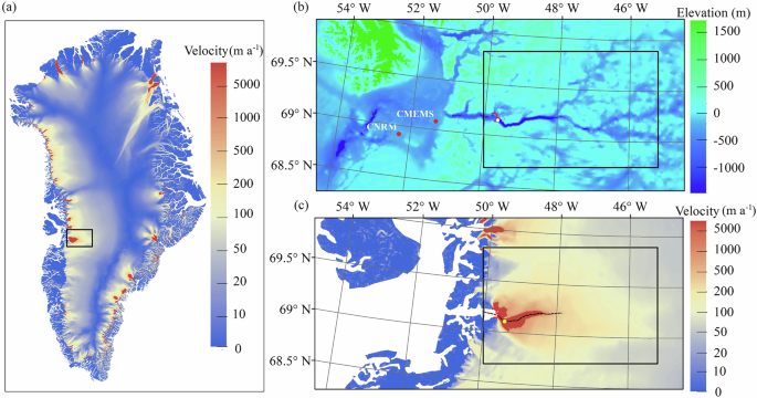
Surface velocity is in the year 2009 from MEaSUREs Greenland Ice Sheet Velocity Map63. The rectangular region in (a) is our model domain, enlarged in (b) with bed elevation map from BedMachine V381, showing the deep trough that defines the main trunk of Sermeq Kujalleq and (c) with the surface velocity. The white circle in (b) is the sampling location of surface runoff (Fig. 4). Red circles in (b) are locations of 250-m-depth ocean temperature modelled by CMEMS and CNRM-ESM2-1. Yellow circle in (c) is the velocity sampling point. Black dashed line in (c) represents the central flowline, which is used to calculate terminus position, defined as the distance along the flowline from the starting point on the left side of flow line to the intersection point of flowline and updated ice front. The glacier terminus position in July 2009 is marked in red near the white circle in (b).
The terminus position of Sermeq Kujalleq was relatively stable between 1950 and 1996 with seasonal fluctuation of about 2.5 km24. Sermeq Kujalleq thickened substantially from 1991 to 1997, and rapidly thinned after 1997. The glacier flowed into a 15 km floating ice tongue before 1997, which then retreated and finally disintegrated in the early 2000s25. Holland et al.6 suggested that warm water originating from the Irminger Sea enhanced basal melting of the ice tongue and triggered its break up in 1997. The glacier has accelerated since 2004 and reached maximum velocities of 17 km yr−1 in 2012 and 201326. The acceleration may have been facilitated by anomalously high surface melting27,28. The glacier then decelerated after 2012 but significant seasonal variability in ice velocity remained29. The thinning rates slowed from 2014, and the glacier thickened and re-advanced between 2016–201930. This deceleration coincided with a period of cooler ocean waters in Disko Bay which connect to Ilulissat Icefjord, when ocean temperatures in Disko Bay’s upper 250 m cooled to those of the mid 1980s30. Joughin et al.31 suggested that the ocean’s dominant influence on Sermeq Kujalleq is through its effect on winter mélange rigidity, rather than summer submarine melting.
The observed historical variability of Sermeq Kujalleq correlated with ocean temperature motivates us to explore the lowering the oceanic thermal forcing by simulating a raised sill at the fjord mouth under a range of climate warming scenarios (SSP2-4.5 and SSP5-8.5) and with historical ocean and air temperatures. Here we simulate the effects of an artificial barrier on the top of the sill at the fjord mouth of various heights on the fjord water properties and glacier basal melt rate, to examine if such an intervention might mitigate retreat and mass loss of Sermeq Kujalleq.
Result
Fjord water temperature and melt rate evolution under different scenarios
We first describe the fjord water temperature evolution in the absence of any barrier. The ocean water near the fjord mouth at 150–250 m depths was relatively cool during the years 2015–2019 (Fig. 2), which led to the modeled fjord water temperature being noticeably lower at the same time (Fig. 3). There is no significant trend for fjord water temperature under SSP2-4.5 for the remainder of the century. However, under SSP5-8.5 there is clear warming trend in the fjord water, especially during 2070–2100, though with seasonal fluctuation and inter-annual variability. Surface runoff greatly increases after 2070 under SSP5-8.5, leading to more subglacial discharge at the grounding line (Fig. 4), which enhances the mixing of plume and fjord water, and results in more melt of the glacier terminus (Figs. 3, 5).

January (top row), April, July and October (bottom row) from CMEMS (location shown in Fig. 1b) for the period 1993–2019, and from bias-corrected CNRM-CM6-1-HR model output (Fig. 1b) for the period 2020–2100 under SSP2-4.5 and SSP5-8.5.

The temperature profiles as a function of depth are shown in Supplementary Fig. 1.
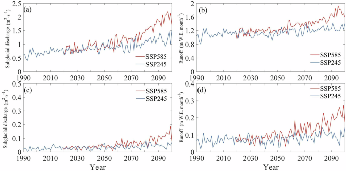
Blue curves represent SSP2-4.5 and red curves SSP5-8.5. Subglacial discharge (a, c) is calculated on a unit grounding line by dividing the total surface runoff over the modelled domain by 5 km, the width assumed of the water sheet released at the grounding line. Monthly total surface runoff (b, d) is over the ice front region from MARv3.11.311 (the white circle in Fig. 1b). Note the differences in the ranges and units of the y axes.
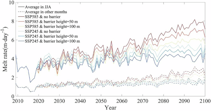
The solid lines represent JJA, and dashed lines other months.
Higher barriers yield cooler fjord water (Fig. 3) and reduced melt rates at the ice front (Fig. 5). We report results with barrier heights of 50 and 100 m. We did explore higher barriers but we do not have confidence in the fjord model simulation of the two-layer exchange flow when the fjord mouth is reduced to less half of its the present-day opening, so we only discuss the 50 and 100 m results compared with no barrier. The 0~250 m depth-averaged fjord water temperature in July 2100 under SSP2-4.5 and SSP5-8.5 drops by ~0.4 °C and ~0.6 °C respectively for every 50 m increase in barrier height. Melt rate at the ice front in summer (June-July-August, JJA) is much larger than in other seasons (Fig. 5), due to the presence of subglacial discharge and higher water temperature.
Glacier evolution under different scenarios
The glacier is subjected to both atmospheric forcing (surface runoff, SMB) and ocean forcings (basal melt rate, ice mélange buttressing effect in calving). We use the moderate SSP2-4.5 forcing (Ex1; Table 1) and the SSP5-8.5 high end forcing (Ex2) outputs from MAR11 and CNRM-CM6−1-HR32. We also explore how ocean and atmospheric forcing compare by keeping ocean forcing under SSP5-8.5 but replacing elements of the atmospheric forcing (Table 1). The three extra forcings are: (i) Ex3: repeated surface runoff in 2010–2019 and SMB under SSP5-8.5, (ii) Ex4: repeated surface runoff and SMB in 2010–2019, (iii) Ex5: repeated surface runoff and SMB in 1990−1999. We also do another experiment (Ex6) using repeated ocean forcing in 1993–2002 (cool ocean) and repeated surface runoff and SMB in 1990–1999.
Figure 6 shows that modeled ice front position in July retreats in response to different atmospheric and ocean forcings in the experiments (Table 1). More surface runoff boosting the development of surface crevasses, increases ice front calving frequency, intensifies glacier retreat, and also yields more subglacial discharge thus enhancing the basal melt rate at the ice front. The fjord water temperature increases with warmer ocean water near the fjord mouth, causing more melt at the ice front. Meanwhile, the ice mélange inside the fjord gives less buttressing to the glacier terminus as fjord water warms (Eq. (5)). In general, the modeled glacier terminus retreats more with warmer atmospheric forcing (more surface runoff; less SMB) or warmer ocean temperature forcing.
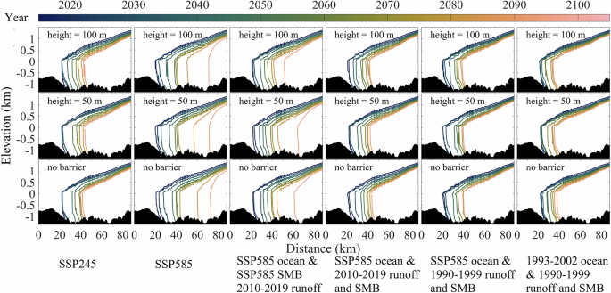
Barrier heights of 100 m (top row), 50 m (middle row) and no barrier (bottom row) under various experiment with oceanic and atmospheric forcing as labeled and shown in Table 1. The distance is in reference to the starting point on the west end of the flowline (Fig. 1c).
With no barrier at the sill, the glacier retreats 19.91 km under SSP2-4.5, and 51.39 km under SSP5-8.5 from 2020 to 2100. Modeled ice front retreats by 22.11 km and 18.94 km with barrier height of 50 m and 100 m under SSP2-4.5, and 51.24 km and 50.66 km with barrier height of 50 m and 100 m from 2020 to 2100 under SSP5-8.5. Therefore, barriers with height up to 100 m make little difference to the glacier terminus retreat under these future climate scenarios.
In Ex3 (3rd column of Fig. 6) surface runoff under SSP5-8.5 is replaced with that from 2010–2019. Comparing Ex3 with Ex2, annual mean subglacial discharge during 2020–2100 has a reduction of 19%, and JJA-mean subglacial discharge during 2020–2100 has a reduction of 35%. The subglacial discharge since 2060 under SSP5-8.5 is significantly higher than that in 2010–2019 (Fig. 4). The subglacial discharge in JJA months during 2060–2100
in Ex3 has a reduction of 48% compared with that under SSP5-8.5. The glacier retreats noticeably less after 2060 in Ex3 than under SSP5-8.5 in Ex2: at 2100 by 40 km, 41 km, and 30 km, with barrier heights of 0 m, 50 m, 100 m. Reduced runoff at the ice front (Fig. 4) since 2060 leads to less ice calving and also contributes to the deduction of glacier retreat in Ex3.
In Ex4 (4th column of Fig. 6) we replace both surface runoff and SMB under SSP5-8.5 for 2020–2100 with repeated data for 2010–2019 (an increase in SMB of 41%), which reduces glacier retreat to 23 km, 20.35 km and 19.77 km, with barrier heights of 0 m, 50 m and 100 m. As with the other experiments, the largest reduction in glacier retreat occurs during 2070–2100. Comparing Ex4 result with Ex3, indicates the importance of maintaining positive SMB to stabilize the glaciers.
Comparing Ex4 with Ex1 without barrier in which they have the similar SMB and runoff in a cold atmospheric scenario but different ocean forcing, we can see the glacier is more unstable and retreats at earlier years on the retrograde slope when subject to warmer ocean thermal forcing. The averaged relative temperature of the inflow ocean water in JJA with respect to freezing point at 250 m depth is 4.6 °C in Ex4 under SSP5-8.5 in the period 2070–2100, while it is 3.4 °C in Ex1 under SSP2-4.5 (Supplementary Fig. 2). This leads to more retreat in Ex4 since 2070 with ocean thermal forcing under SSP5-8.5, although the glacier sits on a prograde slope. Comparing results in Ex5 with Ex6 without barrier leads to a similar finding.
In Ex5 (5th column of Fig. 6) we replace surface runoff and SMB under SSP5-8.5 in 2020–2100 with repeated data from 1990–1999, in which the subglacial discharge is 0.4~0.88 m2·s-1 (48.5% lower) and surface runoff at the ice front is 0.82~1.27 m w.e. month-1 (27% lower). The glacier retreat is again further reduced to 19.49 km, 19.49 km, 18.48 km with barrier heights of 0 m, 50 m, 100 m by 2100.
In Ex6 (6th column of Fig. 6) we replace ocean temperature under SSP5-8.5 in 2020–2100 with repeated data from 1993–2002, but keep the same atmospheric forcing as in Ex5. The glacier retreat is 15.54 km, 12.47 km, 12.91 km with barrier height of 0 m, 50 m, 100 m at 2100. Cooler ocean temperature reduces retreat by a further 20.27%, 36.02%, 30.14% with barrier height of 0 m, 50 m, 100 m relative to Ex5 under the same atmospheric forcing.
The plane view of glacier terminus position evolution in different experiments is shown in Fig. 7. Under SSP2-4.5 forcing the basin retreats from the coastal margins, but under SSP5-8.5 the dramatic retreat along the sub-glacial central trough is much more apparent. This retreat is largely prevented under the conditions in Ex4, 5 and 6. The barrier makes little discernible difference to the pattern of retreat under all experiments. The modeled result using the second best set of parameters are α1 = 0.5, α2 = 0.11, β = 36 (Supplementary Figs. 3 and 4) is close to that using the best set of parameters with differences in retreat of typically 1–6 km by 2100.

The dotted black curve is along the central flowline. The cyan area represents ocean, and the white area represents the ice sheet in 2020.
Discussion
The mean fjord water during the 2080–2100 is 0.5 °C, 1.1 °C cooler with barrier heights of 50, 100 m than that without barrier under the SSP5-8.5 scenario. We investigated the mechanism behind the sill cooling fjord water temperature. The thermal forcing in the inflowing layer over the sill during the 2080–2100 period is reduced by 23% with a barrier height of 50 m and 48% with a barrier height of 100 m relative to the period 2009–2019 with no barrier. The exchange flow changes are much smaller: increases of 2% with a barrier height of 50 m and a decrease of 2% with a 100 m barrier. Hence, the sill largely acts via cooling water temperatures behind the barrier rather than altering exchange fluxes.
Climate-ice sheet intervention aims to tackle the global-scale impact of climate warming on sea level rise. This might be done by local engineered methods at a handful of high-leverage locations, such as ice streams and outlet glaciers that are subject to MISI. Several marine-terminating Greenland outlet glaciers have their terminus in deep fjords that extend far inland of the coast. A leading cause of these outlet glacier retreats is the warm subsurface water into the fjords from the North Atlantic Ocean6,33,34 coupled with vigorous circulation driven by subglacial discharge plumes35, which results in undercutting at glacier termini, and contributed to the loss of almost all Greenland ice shelves, which then leads to widespread glacier retreat and ice flow acceleration. This motivates the exploration of an intervention we simulate here.
There are other issues that would need to be considered before any such intervention were done including social acceptability and political feasibility of the method to the Greenland authorities, and by local communities. These communities exploit the rich fishing that has increased in value as the fresh water supply from beneath the marine-terminating glacier has increased, bring more deep nutrients into the photic zone supporting more phytoplankton36. The warming Atlantic waters have also introduced new commercially important species such as Greenland halibut to the Disko Bay region36,37,38. But any such considerations depend on the question of whether the intervention may feasibly reduce global sea level rise. If the intervention is unlikely to be successful, then the other considerations are moot. Our simulations suggest that an intervention to block warm water intrusion is unlikely to prevent the further retreat of Sermeq Kujalleq. While additional uncertainty remains, and no one modeling study should ever be taken as the final word, these results do suggest that this glacier may have passed the point at which an ocean-focused intervention can save it. Future research into glacial interventions should aim to constrain when different glaciers will pass the point at which interventions will no longer help.
Some uncertainty of the model result comes from the choice of climate forcing data. We only used modeled ocean temperature from CNRM-CM6-1-HR due to its high resolution, after bias-corrected using reanalysis data. Some uncertainty also comes from the use of calving parameterizations, but the comparison between the best and second best set of parameters (Figs. 6 and 7 with Supplementary Figs. 3 and 4) shows qualitatively similar results, but with some difference in the duration of stability on the small prograde bedrock slopes during retreat. This suggests that the results are not particularly sensitive to the selection of the model parameters used. For the treatment of calving in BISICLES, we use a calving parameterization depending on the crevasse penetration depth, which relies on surface runoff. After tuning the parameters, the model did not do a particularly good job of fitting the observed calving front position and motion. But calving is a hard problem for all ice sheet models. Many models struggle to reproduce steady-state calving front positions, let alone the dynamic history of ice front position. Several calving parameterizations have been proposed, including a calving law depending on crevasse depth39, along- and across-flow strain rates (eigencalving)40, and the von Mises tensile stress41. Choi et al.42 evaluated four calving laws over nine tidewater glaciers of Greenland, and found von Mises calving law generally produces terminus change closest to observed, and eigencalving the furthest. More simulations with other calving laws, and other mechanisms for coupling calving to ocean conditions, are needed to improve predictions of glacier dynamics and to improve our understanding of the responsiveness (or lack thereof) of glaciers to interventions.
Some uncertainty also comes from the submarine melting parameterization which we calculate at the vertical face of ice cliff in the fjord model. The plume model result depends on entrainment coefficients, drag coefficient, and turbulent transfer coefficients for heat and salt, etc. Almost all tidewater glacier studies with plume model use the standard set of values (e.g43,45,46,46.). But these coefficients are empirically derived, and have not been validated. For instance, the frictional drag at the ice-ocean interface is parameterized as a quadratic function of the plume speed with a drag coefficient. And the standard drag coefficient value comes from MacAyeal (1985)47 for simulations in which he ignored the Coriolis force. To match observations, Jackson et al.48 suggests that if the basic physics of plume-melt theory are correct, then critical parameters in the plume parameterization must be adjusted. Davison et al.49 varied the turbulence parameters for iceberg melt and showed that larger values of turbulent transfer enhance the impacts of icebergs. In our plume model, the subglacial discharge is assumed to be uniform across the width of water sheet released at the grounding line, hence it does not include entrainment in the across-fjord direction. But for a discrete localized source of subglacial discharge input at the grounding line, the half-conical plume model would be more appropriate based on localized runoff input at the grounding line44 using a different entrainment coefficient.
We find that the maximal monthly melt rate modeled by the fjord model in the summer months (JJA) can be approximated reasonably well by a function that has a nonlinear dependence on inflow water temperature with a power exponent of 0.46–0.55, and a nonlinear dependence on subglacial discharge with a power exponent of 0.23–0.24. The power exponent for dependence on inflow water temperature is about half that is found by Jenkins (2011)43, but he used ambient temperature which will be different from the fjord inflow water temperature that we use. The power exponent of dependence on subglacial discharge is slightly smaller than the 1/3 power found by Jenkins (2011)43. The approximation function we find for melt rate is
under SSP2-4.5 (R2 = 0.87) and
under SSP5-8.5 (R2 = 0.96), where e is the Euler number, m is the maximal basal melt rate at the vertical face of the ice cliff, Qsg represents subglacial discharge, Ta is the inflow temperature water at 250 m depth at the fjord mouth, and Taf is the freezing point of water at depth of 250 m, depending on the salinity of the inflow water. Using the above approximation, a reduction of 48% in JJA-mean subglacial discharge during 2060–2100 in Ex3 compared with Ex2 leads to a reduction of 14% in melt rate. A large fraction of glacial melt rate variability can be thought of as a function of subglacial discharge (e.g35,50.), which comes from surface meltwater. Hence, atmospheric forcing would still be a dominant factor for glacier retreat in the future. However, recent work51 also suggests that seawater intrusions underneath the floating portion Sermeq Kujalleq might contribute considerably to basal melt rates, so perhaps the use of a plume parameterization itself represents a large uncertainty. In addition, we do not use the melt rate at the vertical face of ice cliff in the ice sheet model. Instead, we use equivalent basal melt rate beneath the very short ice shelf. More simulations that implement melt rate at the vertical face of ice front are required to test if this makes significant differences to the modeled glacier dynamics.
The bedrock slope plays an important role in glacier evolution. The modeled glacier retreats in all the experiments we design under either cooler or warmer climates than at present. The fast retreat of the grounding line in the first few decades is partially because the glacier sits on a retrograde slope bedrock, which is consistent with previous studies of MISI (e.g13,52.). The glacier is also reacting to the loss of its ice shelf in 2003, and the warmer atmospheric conditions that appear to remove the winter short section of ice shelf that forms seasonally. The retreat under MISI is characterized by insensitivity to atmospheric forcing, and can only be stabilized by addition of buttressing, or when the glacier rests on a prograde slope at the terminus. This effect can be observed in the simulations where grounding line retreat is slowed on the prograde slope at about 40 km in Fig. 6. Under relatively cool atmospheric forcing (Fig. 6), the glacier does not retreat past this bump in the bed.
Our model appears more sensitive to atmospheric forcing than it is to ocean forcing. But keep in mind that ocean and atmospheric forcing are coupled in our model. Submarine melting of the glacier is influenced not only by ocean temperature coming through the fjord mouth, but also by the subglacial discharge which comes from surface runoff. Ice calving is also impacted by surface runoff in our crevasse depth dependent calving criterion. We may exercise some skepticism about over-interpreting results from this model as the simulations of the historical terminus position was not particularly good. The real glacier is sensitive to ocean forcing as well as atmospheric forcing; but it is not clear whether this sensitivity will continue in the future, even though we know that the central trough is deep and much of the ice discharge in the basin will remain in direct contact with the ocean even though the margins of the basin will retreat away from the ocean inland. So, the terminus will continue to be exposed to deep warm waters even after a large retreat.
Our model is an offline, asynchronous coupled ice sheet-plume model. To better understand the ice-ocean interaction at the glacier terminus, asynchronous or synchronous coupled ice sheet-plume models (e.g46,53,54.) and ice sheet-ocean models (e.g55,56,57.) have been developed over the last decade. Synchronously coupling the ice sheet model with a 3D ocean model is more computationally expensive and more challenging, since ocean models have difficulties accounting for continuously changing ice-margin geometry. But they can simulate both small- and large-scale spatial and temporal evolution of the basal melting beneath ice shelves. However, they require more oceanographic observations which are scarce, and more fjord bathymetry data which are mostly missing or inaccurate than the plume model, which questions the benefit of using computationally expensive 3D models for future predictions.
Conclusion
The barrier scheme we evaluated cannot stop Sermeq Kujalleq retreat in the next few decades under either cooler or warmer climates than present, because the glacier now sits on a submarine retrograde slope bedrock. Our simulations cannot stabilize the glacier even by using the repeated historical runoff and SMB during 2010–2019 or 1990–1999 – which is not very different from the 1960s forcings. However, use of historical atmospheric forcing can largely reduce the retreat especially during the 2070–2100 period, when there is a large increase of surface runoff under SSP5-8.5. This finding aligns with the assessment of the indigenous knowledge holders in Greenland: already before modeling was made, they expressed doubts on the effectivity of the curtain in Ilulissat Icefjord, because of surface melt58.
This result suggests that some glaciers undergoing rapid retreat at present cannot be stabilized under geoengineering scenarios, either by cooling the atmosphere such as with stratospheric aerosols geoengineering12, or by the targeted interventions explored by the barrier simulations here. This conclusion is commensurate with a study of local acceptability of an intervention in Ilulissat58. The locals fear that erecting a barrier would harm their traditional indigenous way of life and economy where fishing and hunting play important role. Other reasons include the distrust in the efficiency and technical feasibility of the curtain, the special value of the Icefjord locally and globally, and the fear of colonialism if a potentially harmful curtain was placed in Ilulissat for preventing global sea level rise. Hence, based on workshops, interviews and informal discussions with over 50 participants in Ilulissat and Nuuk between 2021–2023, there appears to be neither a local or global benefit from making an intervention in Ilulissat. However, there are several other fast flowing and notable outlets for global sea level in Greenland59. While human settlements in Greenland are typically located close to productive fjords38, it is plausible that there are other fjords that would be suitable for field tests, with the consent of Greenland authorities, where there are no local fishing communities relying on the productivity of fjords resulting from the enhanced nutrients supplied by accelerating melt and iceberg discharge. Several of these are in north and northeast Greenland where both oceans and atmospheric thermal forcing is less than for Sermeq Kujalleq. It may be possible to prevent retreat in a MISI regime, such as forecast for Zacharia glacier60. Recent observations of the 79 N glacier61, located next to Zacharia glacier suggest that its fringing ice shelf is being rapidly thinned by warming Atlantic waters. Thus, a barrier may have better potential in stabilizing that glacier than others in Greenland. In any case it appears that Sermeq Kujalleq already passed the tipping point of MISI, and the time for an intervention to make a difference to Sermeq Kujalleq is gone.
Method
Glacier data and Climate Forcing data
The bedrock elevation comes from IceBridge BedMachine Greenland, version 3 at a resolution of 500 m (Fig. 1; Table 2). We take the year 2009 as our initial conditions for simulations. The ice thickness comes from IceBridge MCoRDS L362 at a resolution of 500 m for the year 2009. The observed surface velocity in the year 2009 is from MEaSUREs63 at a resolution of 200 m. The observed terminus positions for the period 2009–2021 are from TermPicks64 and Loebel et al.65 The observed surface velocity for the period 2009–2023 is from MEaSUREs Greenland Ice Velocity, version 466.
The modeled evolution of Sermeq Kujalleq over the 21st century is driven by surface runoff, SMB and ocean thermal forcing. Surface runoff and SMB for the period 1990–2100 are from monthly outputs of regional surface mass and energy balance model MARv3.11.3 with 20 km resolution11. MARv3.11.3 is driven by historical forcing data for the period 2009–2014, and CNRM-ESM2-1 for the period 2015–210067 under SSP2-4.5 and SSP5-8.5 scenarios. Figure 4 shows that almost all surface runoff and meltwater discharge at the grounding line occurs in summer (JJA).
The water in Disko Bay can flow over the 250 m deep sill at the mouth of Ilulissat Fjord. The ocean temperature and salinity above 250 m depth and close to the fjord mouth comes from the monthly reanalysis data CMEMS (https://marine.copernicus.eu/) at spatial resolution of 0.083° × 0.083° for the period 2009–2019, and bias corrected modeled monthly outputs of CNRM-CM6-1-HR for the period 2020–2100. We select CNRM-CM6-1-HR because this has very high resolution for the ocean (25 km) compared with other climate models around Greenland. We do bias correction to the modeled monthly ocean temperature and salinity using the equidistant cumulative distribution functions (CDF) matching (EDCDFm) method. This follows standard procedures in bias correction which tries to account for probability distribution changes, as well changes to mean, between the projection and baseline periods for the modeled variable68. There is an apparent 3-year ocean water cooling period 2016–18 which can be most easily seen at depths greater than 100 m shown by the reanalysis data CMEMS. And there is abrupt ocean water warming, most obvious in January and April, starting in 2019 (Fig. 2), due to switching the ocean forcing data.
Ice sheet model
We model Sermeq Kujalleq using the ice sheet model BISICLES69,70. BISICLES employs a vertically integrated ice flow model based on Schoof and Hindmarsh71 which includes longitudinal and lateral stresses and a simplified treatment of vertical shear stress which is best suited to ice shelves and fast-flowing ice streams.
The ice thickness h and horizontal velocity u satisfy a two dimensional mass transport equation
and two dimensional stress-balance equation
where a is surface mass balance (SMB), M is the oceanic met rate only applied to the ice shelf bottom, φ is the stiffening factor, (hbar{mu }) is the vertically integrated effective viscosity, (dot{{{boldsymbol{epsilon }}}}) is the horizontal strain-rate tensor, I is the identity tensor, ({rho }_{i}) is the ice density, g is gravity acceleration, s is the surface elevation69. The submarine melt rate in Eq. (3) beneath the ice shelf of Sermeq Kujalleq is not estimated by a simple parameterization, but using the output of a fjord model described later.
BISICLES employs adaptive mesh refinement to obtain fine spatial resolution in fast flow region and coarse resolution in low flow region. We use 500 m in the region of grounding line, and 1 km upstream and 2 km far inland (Supplementary Fig. 5).
We use a crevasse-based calving criterion that calves ice where the crevasse penetration depth, ds, is greater than upper surface elevation, which is based on the idea that the downglacier velocity gradient and the ice elevation above the waterline are the primary controls on glacier terminus position72. We also include the effects of surface runoff in the opening of crevasses and the rigid ice mélange in suppressing calving on Jakobshavn Isbræ73,74. Then ds is estimated as
where S is the magnitude of tensile stress and R is surface runoff; α is a tuning coefficient, which is linearly dependent on ocean temperature to represent the buttressing of ice mélange in the fjord:
where To is the average water temperature above 250-m-depth in the Ilulissat Fjord, μ and ({sigma }^{2}) are mean and variance values of To during the simulation period respectively; β is a tuning parameter of runoff. The parameters α and β are tuned to best reproduce the observed calving front position for the period 2009–2019.
A linear Weertman sliding relation is used for grounded ice to define the basal friction:
where ({{{boldsymbol{tau }}}}_{b}) is the basal shear stress, ({{{bf{u}}}}_{b}) is the basal velocity, and C is the basal friction coefficient.
The basal friction coefficient C and the stiffening factor φ (Eq. 4) are fixed throughout the simulations and obtained simultaneously by solving the inverse problem70 with bedrock topography, ice thickness and ice surface velocity in the year 2009 (Table 2).
Fjord model
We consider an elongated fjord roughly representative of the geometry at Illulissat Icefjord in front of Sermeq Kujalleq (Fig. 1). This picture (Fig. 8) is inspired by the detailed observational and modeling description of Ilullissat circulation in Gladish et al.7 That paper described a fjord whose properties and internal overturning circulation are essentially determined by two competing plumes: at the seaward end, dense inflowing water cascades over a shallow sill to fill the deep basin of the fjord, while at the glacier end, buoyant meltwater creates a buoyant upwelling plume. Our model is customized to capture these specific dynamics.

The red bar at the left side of (a) represents the barrier; the exchange flow details over the sill or barrier are shown in (b).
In our model, the seaward end of the fjord consists of a shallow sill, while the landward end is the ice sheet terminus. At the seaward end, a two-layer exchange flow with the surrounding ocean results in dense water entering the fjord at relatively shallow depths. This inflow is denser than the ambient fjord properties and thus it cascades down the spillway slope at the back of the sill as a negatively buoyant turbulent plume. When this plume reaches its level of neutral buoyancy, its outflow spreads horizontally into the ambient fjord waters. At the glacier end of the fjord, fresh subglacial discharge triggers another plume, this one positively buoyant. The glacier plume entrains ambient deep water from the body of the fjord; the heat from this deep water triggers melting at the ice face, and the mixture of entrained water and ice melt is upwelled and then discharged into the ambient shallow layers of the fjord. As the two outflows spread out horizontally at their levels of neutral buoyancy within the fjord, they displace ambient water masses up and down to maintain a stable stratification. The vertical stratification of the fjord is thus determined by the balance between entrainment and outflow of these two plumes, and our model therefore consists of three coupled 1D models: two plume models (a positively buoyant one at the glacier face and a negatively buoyant one on the sill spillway), that communicate with each other via a vertical advection-diffusion equation for keeping track of the ambient fjord properties in the middle.
In our simplified model, the ambient vertical profiles of water properties within the fjord are determined by the solution to the 1D vertical advection/diffusion equation, with source and sink terms corresponding to the entrainment and outflow of the two plumes, and an additional term to account for parameterized iceberg melt. The evolution equations for conservative temperature ({{Theta }}) and absolute salinity S in depth z and time t are thus:
where wf is the fjord upwelling velocity; us and ug are the outflow velocities from the sill and glacier plumes, respectively, with associated outflow temperature and salinity given by Θs, Θg, Ss, and Sg; mi is the iceberg melt rate, described below; Θi=−L/cp is the equivalent water temperature of frozen ice, where L is the latent heat of melting and cp is the specific heat of seawater (the salinity of frozen glacier ice is assumed to be 0); l is the fjord length from glacier to sill; and κ = 10-3 m2s-1 is a vertical diffusivity added to stabilize the problem.
The fjord upwelling velocity is computed by integrating the net entrainment and outflow of the two plumes:
where es and eg are the entrainment rates of the sill and glacier plumes, respectively, and zb is the depth of the fjord bottom. Note that, while we do not explicitly impose the boundary condition that w=0 at the sea surface, we implicitly enforce this condition by the fact that both plumes conserve mass, such that the integrated entrainment and outflow terms balance.
The two plumes follow the turbulent buoyant plume model of refs. 43,75. They are governed by four equations describing the conservation of mass, momentum, heat, and salt. At the ice face the plume model uses the simplified two-equation melt model from Jenkins43. We use the parameter values from Table 1 of Jenkins43 for both plume models. For the sill plume we disable melting and integrate the plume model downwards along the spillway, with an assumed slope of 3.4°. The initial conditions for the sill plume are derived from the sill exchange model, described below. For the glacier plume, we integrate the plume equations upwards along the vertical ice face starting from an initial subglacial discharge. The plume model continues integrating beyond the neutral buoyancy depth so as to capture the magnitude of dynamic overshoot; this overshoot is used to compute a vertical spreading function which determines the depth distribution of the plume outflow into the rest of the fjord (see Supplementary Information).
The final component needed by our model is an expression for the exchange flow over the sill that connects the fjord with the surrounding ocean. This two-layer critical flow provides the starting boundary conditions for the dense sill plume. For this purpose, we use a theoretical treatment for critical exchange flows inspired by Farmer and Armi76. The geometry of the two-layer exchange flow is shown in Fig. 4b. For any given value of the interface height, we can define layer thicknesses h1 and h2, along with average densities ρ1 and ρ2 given by the properties of either the fjord profile (for the outflow layer 1) or the external ocean (for the inflow layer 2), averaged over the appropriate depth range. The densities can be used to compute a reduced gravity, g’=Δρ/ρ0. Our unknowns are u1 and u2, the exchange velocities. To conserve the overall mass of water in the fjord, the exchange velocities are related by,
where q0 is the net barotropic flux out of the fjord (this term is necessary to balance the inflowing ice, but in practice it is quite small in comparison to the exchange fluxes). The condition that the flow over the sill must be a hydraulically controlled critical flow, as observed by Gladish et al.7 can be expressed as:
where G is the composite Froude number of the exchange flow, composed of the Froude numbers for the individual layers F1 and F2. Using mass conservation to express u1 in terms of u2, we can then rearrange the above equation to form a quadratic equation for u2:
We test all possible interface heights between the top of the sill or barrier and the sea surface, and compute u2 (and thus u1) for each of them. Finally, by making the assumption that the system will maximize entropy production when the magnitude of the exchange flow is maximized, we can select the interface depth that separates the inflow and outflow layers, thus completing the problem. If a barrier is placed at the sill the calculation of exchange flow is the same, except confined to a shallower region above the barrier.
We assume the runoff at the glacier surface is all discharged at the grounding line, which drives the plume near the ice front. We assume the subglacial discharge comes out from the grounding line through a 5 km wide water sheet. We use the subglacial discharge per kilometer (Fig. 4). The modeled melt rate at the ice front given by the fjord model is at the vertical cliff face of the ice terminus. It primarily depends on fjord water temperature and subglacial discharge which drives circulation. Melt rate can be increased by an increase in either variable, although it increases linearly with fjord water temperature and only sub-linearly with subglacial discharge (e.g35.). We convert the maximum melt rate at the vertical ice front to an equivalent melt rate beneath the seasonal ice shelf using the grid cell size and ice thickness ratio.
The fjord model we use is adapted specifically for the conditions in Ilulissat Icefjord: the glacier end of the fjord is a nearly vertical ice cliff, justifying the use of a vertical plume model; the fjord itself is narrow and choked with icebergs, inhibiting the formation of eddies or large-scale cross-fjord structure; and the entrance has a relatively shallow sill, with two-layer hydraulically controlled exchange flow occurring in the space above the sill7. This model would be inappropriate to use for fjords where these conditions are not met, for example if the sill is deep enough to permit three-layer or more complex exchange flows (e.g77.). We acknowledge that this fjord model is simple and neglects important fjord parameters including the effects of mixing at sills the earth’s rotation, and fjord-wide circulation. Slater et al.45 suggests plumes can drive an energetic fjord-wide circulation which effectively doubles the glacier-wide melt rate compared to estimates of melting within plumes alone, and melting driven by fjord-scale circulation should be considered. However, the primary goal of the fjord model is to modify an ocean temperature boundary to produce a thermal forcing on the glacier and not to recreate fjord circulation perfectly. This is like other glacial fjord box models and parameterizations (e.g78,79,80.). Nevertheless, we would welcome 2D and 3D ocean general circulation models, off- or on-line coupled to an ice sheet model to repeat the work and compare with our result.
Initialization, calibration and coupled model scheme
We assume that the bedrock topography beneath the ice sheet is unchanged in decades. We used bedrock topography in the year 2017, ice thickness and velocity in 2009 (Table 2) to provide a state in 2009. The initialization and calibration was performed as follows.
-
1.
We solved the inverse problem for basal conditions (Eq. 7) and stiffening factor following Cornford et al.70 Supplementary Fig. 6 shows the discrepancy between observed velocity field63 and the velocity derived from the inversion.
-
2.
Using φ and C from the inversion of Step 1, we performed a surface relaxation for 0.1 years to reduce errors caused by inconsistencies in data coverage and observation time.
-
3.
We ran the fjord model over the 2009–2019 period to produce water temperatures inside Ilulissat Fjord needed for Eq. (5), and the monthly basal melt rate at the ice front, forced by the water properties and velocity at the fjord mouth, and subglacial discharge through the grounding line.
-
4.
We used many individual decade simulations to determine the parameters α1, α2 and β, which represent mélange buttressing and crevasse depth sensitivity to surface runoff. We minimized that mismatch between observed and modeled monthly calving front position during the period 2009–2019.
The best set of parameters are α1 = 0.6, α2 = 0.15, β = 34 (Fig. 9). The second-best set of parameters are α1 = 0.5, α2 = 0.11, β = 36 and these we use in a sensitivity analysis of glacier response to parameter selection. The modeled timings of maximum extent and minimum extent each year are in satisfactory agreement with observations, and the error distribution shows a single minimum (Supplementary Fig. 7). The glacier terminus reaches maximum extent with slowest ice velocity in December and January, and minimum extent with highest velocity between June and August. The modeled calving front shows net retreat with seasonal fluctuations, and retreats 3.5 km from summer of 2009 to the summer of 2015, which is consistent with observations. Ocean temperature cooling from 2015 to 2017 (Fig. 2) triggered substantial advance of calving front (Fig. 9), demonstrating the sensitivity of our ice mélange buttress parameterization to ocean forcing. Data from after 2019 were not included in the parameter fitting, but the model captures the calving front position and velocity reasonably well (Fig. 9), and better than the second-best parameter set (Supplementary Fig. 8).

a Observed calving front position (black circles) from TermPicks66, compared with simulated calving front position (red line). Observed calving front position in 2009–2019 are used for parameter tuning in the calving parameterization. b Measured monthly mean ice flow speed68 near ice front (black circles) taken at the yellow circle location in Fig. 1c, compared with modeled speed (red line). c Residuals (modeled minus observed) of monthly calving front position. d Residuals (modeled minus observed) of monthly velocity.
We use asynchronous coupling between the ice sheet model and the fjord model for the projections from 2020 to 2100. The water temperature inside Ilulissat Fjord and basal melt rate under the ice shelf from 2009 to 2100 come from the fjord model. The time step of the fjord model is 1/4 day, while that of BISICLES is one month. The monthly basal melt rate is used for forcing the ice sheet model. The ice sheet model yields the glacier terminus position change, which corresponds to the fjord length change. Fjord length essentially controls how quickly fjord properties can change in response to changes in the incoming fluxes. Small changes of fjord length have little influence on the modeled fjord water properties. We chose to update the fjord length every 10 years to balance computation cost and accuracy of the evolution of glacier terminus, but we use the modeled monthly basal melt rate from the fjord model to drive the ice sheet model.
We designed the following scheme for coupling the ice sheet model BISICLES and the fjord model for the period 2020–2100:
-
1.
We repeated the year 2020 drivers for 3 years to spin-up the fjord model. We then run the fjord model for the first decade: 2020–2029.
-
2.
We applied the monthly average of modeled water temperature and basal melt rate from the fjord model to the ice sheet model BISICLES, and run BISICLES for 10 years. This produced the modeled glacier velocity and the evolution of glacier geometry including glacier terminus position.
-
3.
We updated the length of fjord with the last glacier terminus position from step 2, then repeated steps 1 and 2 for the next decade. Each new decadal simulation is preceded by a 3-year spin up of fjord model with repeated forcing from the last year of the last decade.
Responses