Advanced machine learning for regional potato yield prediction: analysis of essential drivers

Introduction
Ensuring accurate predictions of potato yield is vital for addressing the challenges of food security and adapting to global climate change1. With potatoes being a staple crop in many regions, reliable yield forecasts empower farmers to optimize their practices, enhance economic stability, and contribute to global food security. Traditional methods in agricultural yield prediction, such as statistical regression, primarily utilize historical yield data and climatic variables to forecast outcomes2. These conventional statistical approaches often struggle with non-linear and complex environmental interactions, limiting their ability to accurately predict crop productivity3,4. In addition, process-based models, which simulate the biological and physical processes affecting crop growth, offer a detailed mechanistic understanding. However, these models require extensive parametrization and are highly sensitive to the accuracy of these parameters5. The assumptions underlying these parameters, such as those simplifying genotype influence, can restrict the applicability of models in dynamic agricultural environments, as yield is affected by many genes6. The challenge of calibrating and validating these parameters across different crops and locales often leads to a compromise between model complexity and operational utility5. Moreover, regional crop models are computationally expensive due to their complexity and the need to capture spatial variability in soil and climate conditions. The application of process-based models is further limited because they require detailed data on management practices, which are often unavailable, forcing reliance on scenario-based assumptions7. The recent accelerated use of machine learning (ML), along with readily available Earth observation data, has led to improved yield predictions8. Our study extends the frontier of agricultural forecasting by integrating machine learning techniques that harness a comprehensive array of data streams. The adoption of these techniques is crucial for addressing the limitations of process-based modeling, especially at regional scales, and for overcoming the constraints of traditional statistical methods, which typically aim to estimate underlying data distributions based on predefined assumptions. Machine learning models, in contrast, do not rely on such assumptions and are more capable of capturing nonlinear and complex interactions among numerous environmental variables that affect crop yields. This allows machine learning approaches to offer more flexible in the face of such complexity9,10.
Earth observation data, integrated with statistical methods and machine learning techniques, has been used to predict crop yields both globally and within Canada11,12,13. The Canadian Crop Yield Forecasting (CCYF) system is a geospatial modeling tool that employs statistical methods to predict yields at the Census Agricultural Region (CAR) scale across Canada for most crops. While CCYF has shown to be effective in predicting yield a month before harvest, its performance needs improvement, particularly in Central Canada and the Atlantic provinces14. The Atlantic province of Prince Edward Island (PEI) plays a crucial role in Canada’s agriculture, particularly in potato production, which is a key component of both local and national markets. PEI is one of top producer of potatoes in Canada, with its potatoes being exported to over 40 countries globally. In 2019, PEI dedicated 85,500 acres to potato farming, representing the largest share of potato acreage in Canada15,16. The island’s agricultural success is largely due to its unique climate and committed farming practices, which are well-suited for potato cultivation. However, because PEI relies on non-irrigated fields, predicting yield is challenging due to dependency on natural water sources and rainfall patterns. This unpredictability highlights the need for advanced predictive tools to provide reliable yield forecasts, aiding in better resource planning and management strategies17,18. Here, we aim to address the shortcomings in yield prediction in the Atlantic provinces by utilizing soil, climate, and Earth observation datasets19,20,21, and employing a novel method. Our method diverges in two key aspects: 1) it is applied specifically to potatoes-a new crop focus utilizing data at the postal code level, and 2) it utilizes advanced machine learning techniques rather than the traditional statistical methods11,22,23. ML was previously employed for potato yield prediction in Atlantic Canada using limited field-scale data, and it was found that large datasets are essential for achieving meaningful results24. Our localized approach at the postal code level provides detailed insights into the main drivers of yield prediction and allows for the extrapolation of our findings to the provincial level, underscoring the significance of such granular data in agricultural research. This approach provides a novel, localized perspective that contrasts markedly with broader-scale agricultural studies25. To demonstrate our model’s performance, we have utilized over three decades of yield data at the postal code level from Prince Edward Island (PEI), a leading potato production province in Canada.
Our study employed various linear, tree-based, and ensemble models to predict crop yields at the postal code level in PEI. To ensure both robust and accurate model predictions, we implemented two preprocessing techniques, combined with Grid Search and cross-validation across different model configurations and pipelines26. Robustness was evaluated by testing the model’s consistency and performance stability across different data subsets, while accuracy was measured by comparing predictions to observed yields using the Mean Squared Error (MSE) as metric27. Notably, different models identified various key predictors, with water stress emerging as particularly significant due to PEI’s reliance on non-irrigated fields. This variability highlights the necessity for localized predictive tools that are tailored to specific agricultural contexts, underlining the importance of advanced modeling techniques in improving yield forecasting accuracy28.
Results
Correlation analysis between yield and agroclimatic features
We conducted an analysis to uncover the relationships between crop yield (measured in tonnes per acre, t/ac) and various derived input values. For each postal code, we generated numerous features from the primary data collected. For a complete list of all features and their descriptions, refer to Supplementary Table S1 in the supplementary materials. In total, we derived 58 features from the three main data sources, which were then categorized into climate, soil, and NDVI groups. Figure 1 displays a heatmap of the pairwise Spearman correlations among various features. The colors in the heatmap represent the strength of these correlations, providing insights into the environmental and agricultural dynamics at each postal code level, specifically focusing on crop yield in t/ac.

The colors on the heatmap denote the strength of these correlations, providing valuable insights into the interactions between environmental and agricultural factors. Figure created using R.
We assessed the correlation between various features and average crop yield. The average yield, referred to as Yield Avg, is calculated as the mean yield across all reported years for each postal code. Unlike Yield, which represents the average potato yield for a specific postal code in a particular year and serves as the target variable, Yield Avg reflects the overall average yield across all available years for each postal code, capturing long-term yield trends rather than annual variations. We found that base saturation demonstrated a weak positive correlation of 0.150 with average yield, suggesting that higher levels of soil base saturation, which indicates soil fertility, are beneficial for crop productivity. Additionally, late-season rainfall showed a weak positive correlation of 0.260, emphasizing the importance of water availability during critical growth stages. The start, middle, and end of season minimum temperatures had mixed correlations with yield: early season temperatures showed a very weak negative correlation of −0.092, while mid and late-season temperatures were positively correlated at 0.134 and 0.206, respectively, highlighting that warmer temperatures later in the growing season contribute positively to crop yield. Furthermore, the soil water stress index (SI) showed moderate positive correlations at the start, middle, and end of the growing season (0.399, 0.341, and 0.364). This indicates that effective water stress management, reflecting the balance between water availability and crop demand, is crucial for maximizing yield.
The correlation values obtained for total sand, silt, and clay content with both average yield in PEI highlight intriguing interactions between soil composition and potato yields, under conditions where there is no irrigation and crop rotation is practiced. Sand content shows a moderate positive correlation 0.336 with the average yield, suggesting that the well-drained nature of sandy soils might be particularly beneficial for potatoes, which are prone to diseases in waterlogged conditions. Conversely, both silt and clay content exhibit negative correlations −0.310, −0.320, which could indicate that while silt may impede drainage slightly, the high clay content might lead to poor soil aeration and drainage, counteracting the benefits of its higher nutrient retention capacity. These findings highlight the importance of adopting soil-specific agricultural practices in PEI. For sandy soils, enhancing soil organic carbon (SOC) through the addition of organic matter is crucial for improving water retention and nutrient availability, while in clay-rich soils, amendments can be used to improve structure, aeration, and drainage29,30,31. This nuanced understanding of soil properties and their impact on crop yields is crucial for developing sustainable agricultural policies and practices that optimize the diverse soil environments specific to regions like PEI.
Additionally, some unexpected correlations were observed. For example, the average range of NDVI showed a negative correlation of −0.011, indicating that greater variability in NDVI might be linked to lower yields, possibly due to inconsistent plant growth. Similarly, the peak NDVI had a weak positive correlation of 0.14, suggesting that higher peaks in NDVI correspond to higher yields. These correlations highlight the intricate interactions between climatic, soil, and plant growth factors and their collective impact on yield. Understanding these relationships aids in refining predictive models and improving agricultural practices for better yield outcomes.
Predictive modeling of crop yield at the postal code level
Our dataset, which integrates crop yield, climate, soil, and NDVI data, facilitated the development of predictive models aimed at understanding crop yield at a regional level. To ensure the accuracy of our predictions, we explored a diverse array of machine learning models that are adept at capturing both straightforward and intricate interactions within the data32. We constructed and evaluated eleven different models, categorized into linear, tree-based, and ensemble models, to predict crop yield for each year and postal code. For the linear models, such as Lasso, Ridge regression, Bayesian Ridge, and Orthogonal Matching Pursuit, we focused on feature selection and regularization to manage simpler relationships and reduce overfitting. The tree-based models, including Decision Tree and Random Forest, were selected for their capability to deal with non-linear relationships and complex data interactions. Additionally, we utilized ensemble methods like AdaBoost, Gradient Boosting, and others involving stacking, voting, and bagging techniques, which combine the strengths of multiple models to enhance prediction accuracy and model stability. To optimize the learning process, we applied two preprocessing techniques: polynomial transformations and power transformations33,34. These techniques are designed to capture different dimensions of the underlying patterns in the data, thereby improving the models’ performance in yield prediction scenarios.
To evaluate model performance, we utilized the mean square error (MSE) metric and cross-validation techniques27. Considering the temporal dependency of the yearly data points, cross-validation was employed to ensure that models were trained on past data and tested on future data. We implemented five splits or folds. After training the models on the training set, their performance was evaluated on the test set. The cross-validation results indicated that power transformation preprocessing technique was better than polynominal transformation as shown in Table 1. The cross-validation results indicated that the power transformation preprocessing technique outperformed the polynomial transformation, as shown in Table 1. While polynomial transformation generates new features based on the interaction between existing ones, it can amplify noise and overfit the model in some cases. In contrast, power transformation makes the data more Gaussian-like, stabilizing variance and reducing skewness, which is particularly effective for features with non-normal distributions. This leads to more robust models and improved prediction accuracy, especially in scenarios where non-linear relationships exist. Random Forest achieved the best performance, with an MSE of 0.014 (t/ac)2, a root mean square error (RMSE) of 0.119 (t/ac), and an R2 of 0.99. Gradient Boosting also performed exceptionally well, with an MSE of 0.037 (t/ac)2, an RMSE of 0.191 (t/ac), and an R2 of 0.99 (see Table 1). Among the linear regression models, Ridge Regression showed a respectable performance with an MSE of 0.410 (t/ac)2 and an R2 of 0.93, although it was not as effective as the tree-based models.
Ensemble techniques demonstrated improvements over linear models by combining the strengths of multiple models. The Stacking technique, which integrates the predictions of the best-performing tree-based and ensemble models (Random Forest, Gradient Boosting, and AdaBoost), achieved an MSE of 0.240 (t/ac)2, an RMSE of 0.489 (t/ac), and an R2 of 0.96. This approach involves training several models and then using another model to optimally combine their predictions. The Voting Ensemble also showed strong performance, with an MSE of 0.265 (t/ac)2, an RMSE of 0.515 (t/ac), and an R2 of 0.95. This method aggregates predictions by averaging (for regression), enhancing overall predictive performance by leveraging the diverse strengths of each model. However, ensemble techniques might have slightly less performance than Random Forest due to the additional complexity and the potential for overfitting in their process. Overall, the results indicate that Random Forest and Gradient Boosting Regressors provided the most accurate predictions for crop yield. Feature selection and transformation techniques used in the preprocessing steps were crucial in managing overfitting and capturing the dependencies in the data effectively.
Model error analysis by postal code
A granular analysis is provided to explain model errors in predicting crop yield at the postal code level, as shown in Fig. 2. This detailed analysis provides a clearer understanding of how different models perform across various geographic locations. Panel A illustrates the average difference between observed and predicted yields for each postal code, identifying the best-performing model for each location. The error varies across postal codes, with power transformation preprocessing consistently yielding the best results. Larger errors are associated with postal codes having fewer data points, which is often due to the density of agricultural areas. Postal codes with more farmers reporting data or higher agricultural activity tend to have lower errors, whereas postal codes encompassing more urban areas with less cultivation tend to have larger errors. Panel B categorizes yields into low, medium, and high values, calculated based on the 25th percentile (low), 75th percentile (high), and the interquartile range (medium). Generally, models tend to overestimate high yields, underestimate low yields, and are fairly consistent around zero for medium yields. This trend occurs because the dataset exhibits more medium values and fewer extreme values. Random Forest and Gradient Boosting models exhibit the best consistency across these categories, making them the most effective algorithms for yield prediction across all postal codes. This comparison offers insights into how model performance varies across different levels of crop yield, revealing which models are more robust and reliable across varying agricultural scenarios. Panel C presents scatter plots comparing observed versus predicted yields. Tree-based algorithms, particularly Gradient Boosting and Random Forest, demonstrate superior performance with less variation. On the other hand, models like Lasso and Ridge regression, as well as the Bagging technique, show lower performance and greater variation in the scatter plots. This analysis underscores the importance of selecting the appropriate model and preprocessing technique to achieve the most accurate yield predictions.
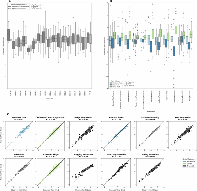
A Box plot showing the average difference between observed and predicted yields for each postal code, with preprocessing techniques distinguished by color. B Box plot comparing prediction errors of different models across low, medium, and high yield categories, providing insights into model performance under varying yield conditions. C Scatter plots showing the relationship between observed and predicted yields for various models, categorized into linear, tree-based, and ensemble models. Figure created using R.
Overall, these plots highlight the effectiveness of tree-based models, especially when using power transformation preprocessing, in accurately predicting crop yields across different postal codes. The results at the postal code level are consistent with the general findings, reinforcing the reliability of the tree-based models in diverse regional conditions.
Key features influencing crop yield identified by the model
In this section, we identify and rank the most influential predictors of crop yield based on our model analyses, as illustrated in Fig. 3. The analysis revealed a strong correlation between temperature-related variables and yield metrics, emphasizing the critical role of climatic conditions in agricultural productivity. Similarly, the relationship between rainfall and soil water retention highlighted the importance of efficient water usage. NDVI showed significant correlations with yield and growth rate, underscoring its utility in remote sensing for crop monitoring and yield forecasting. The bar plot in Fig. 3A ranks features by their average absolute SHAP values, identifying the most impactful variables in our model. For instance, the start of the season water stress index (SS SI) and the NDVI Fourier transform cosine (NDVI FT Cos) emerged as top predictors of crop yield. The SHAP summary plot in Fig. 3B further details the contributions of each feature, with color gradients indicating feature values and point density representing the concentration of SHAP values. Our analysis included aggregating SHAP values and feature importance scores across top-performing model predictions and preprocessing techniques, providing a comprehensive overview of the most influential factors. Features like temperature and rainfall, while directly affecting yield, also set the overall growing conditions. Maximum temperature during the growing season (Temp Avg Max) and accumulated rainfall (Rainfall Accum) were significant predictors, with high temperatures potentially causing heat stress and sufficient rainfall being crucial for soil moisture. The SHAP analysis revealed that certain features were highly influential on yield, despite not having high correlations in traditional analysis. For example, base saturation and very fine sand ranked 16th and 20th in SHAP analysis Fig. 3, but had low correlation coefficients of 0.15 and −0.03, respectively Fig. 1. Note that the very fine sand is a portion of total sand with smallest diameters. The models are effectively capturing these relationships, helping to accurately predict yield by leveraging these factors. These factors likely affect soil nutrient availability and water retention, indirectly influencing crop yield. Some features with high SHAP values showed low correlations in traditional analyses, indicating their subtle yet critical role in yield determination. NDVI metrics, for example, demonstrated strong predictive power in SHAP analysis, which may not be fully captured by simple correlation measures.

A Describes the bar plot showing feature importance based on average absolute SHAP values. This plot ranks features by their overall impact on the model output. B Describes the SHAP summary plot for the top 25 features. This plot provides a detailed view of how each feature contributes to the model’s predictions, with color indicating the feature value and density indicating the concentration of SHAP values. C Displays the Spearman correlation test results for the top 15 features, illustrating the correlation between these features and yield values. Each scatter plot shows the relationship between a specific feature and yield, with different colors representing different sources such as climate, crop, NDVI, and soil. Figure created using Python.
To further explore these relationships, we constructed scatter plots for various features, highlighting their influence on yield predictions, as illustrated in Fig. 3C. In these scatter plots, features like water retention at 0 KP appear as vertical dots, indicating discrete values. This pattern suggests that water retention measurements at specific pressure levels are categorized into distinct groups rather than forming a continuous range. This is likely due to the nature of soil water retention characteristics being measured at fixed pressure points, which are critical for understanding soil moisture dynamics and their impact on crop yield. The ρ values, representing Spearman’s rank correlation coefficients, indicate the strength and direction of the relationship between each feature and yield. For instance, a ρ value of 0.20 for soil saturation index (SI) suggests a moderate positive correlation, meaning that as SI increases, the yield tends to increase likely because higher soil saturation means better water availability for crops, promoting growth. Similarly, the ρ values for NDVI average range (NDVI Avg Range) and Fourier transform sine (NDVI FT Sin) components, which are 0.39 and 0.00 respectively, reveal interesting insights. The positive ρ for NDVI Avg Range indicates that this component is significantly correlated with yield, reflecting the importance of seasonal vegetation dynamics. In contrast, the ρ value of 0.00 for NDVI FT Sin suggests no correlation, indicating that this feature does not influence yield predictions. Additionally, features such as temperature and rainfall also exhibit notable correlations. For example, the ρ value of 0.16 for average maximum temperature (Temp Avg Max) implies a positive correlation, suggesting that while higher temperatures can benefit crop growth, the relationship is not strongly linear and other factors may moderate this effect. Conversely, a feature like growth rate, despite showing low traditional correlations, has a high SHAP value indicating its nuanced role in yield determination by affecting soil nutrient availability and water retention indirectly. These scatter plots, combined with SHAP analysis, offer insights not just into correlation but also into how features contribute to model predictions. For example, while features like water retention at specific pressure points show vertical clusters (indicating discrete measurements), SHAP values help explain how these features influence the model’s output, either positively or negatively. This is particularly useful for understanding model behavior, where traditional correlation analysis might not capture a feature’s actual impact on predictions.
These scatter plots and correlation values help us understand the complex interactions between different agroclimatic and soil features and crop yield. By visualizing these relationships, we can identify which features have the most substantial impact on yield predictions and refine our models accordingly. Moreover, the presence of no negative SHAP values across the models underscores that the identified features consistently contribute positively to yield predictions, enhancing the overall robustness and reliability of the models. Notably, while early-season NDVI offers valuable insights, its effectiveness wanes later in the season due to saturation. Incorporating additional indicators such as climate data could mitigate this limitation, potentially increasing the predictive power and accuracy of our the models.
Discussion
Predicting crop yield from climate, soil, and NDVI data is a major advancement for agricultural science, especially for regions like PEI and broader Canadian agriculture. Reliable models that link environmental and biological data to crop performance can greatly benefit precision farming, optimize resource use, and enhance food security. These tools offer an efficient and cost-effective alternative to traditional field trials and manual yield estimations, allowing farmers and policymakers to make better-informed decisions for sustainable agriculture35.
Our study demonstrated the effectiveness of modern machine learning models, particularly tree-based models like Random Forest and and ensemble models like Gradient Boosting Regressors, in predicting crop yield from a comprehensive dataset. By integrating climatic variables, soil properties, and NDVI data, our models achieved high accuracy and robustness across different environmental conditions. Our NDVI dataset from MODIS is available every 16 days, and we divided the growing season into three distinct phases to capture NDVI data during key growth stages. NDVI typically peaks during the maturation phase and then stabilizes until harvest. Although cloud cover may sometimes obscure satellite passes, the 16-day intervals provide multiple opportunities to capture the peak NDVI. By focusing on this peak and the trend leading up to it, our model enables accurate predictions of yield potential well before harvest, allowing for timely insights into crop performance. Importantly, our results matched or exceeded the accuracy of similar studies in potato yield prediction, demonstrating coefficients of determination (R2) and root mean square errors (RMSE) comparable to or better than those reported in other research (i.e., RMSE ranging from 1.76 to 3.94 t/ac and R2 ranging from 0.49 to 0.86)1,13,24,25. We note that the yield prediction discussed in this paper was based on data from the entire growing season and did not use partial-season inputs to assess how early and accurately the model could predict yield before harvest. Such an assessment can now be made by integrating these advanced models into the Canadian Crop Yield Forecaster (CCYF) for real-time application. The CCYF, as detailed in11, relies on a linear model and leverages short- and medium-term climate forecasts from Environment Canada or similar services to fill gaps in growing season data, such as precipitation, temperature, and GDD. For data that may not be available in near-real-time, such as NDVI, the models can either interpolate missing values based on prior seasonal trends or substitute alternative indices, such as vegetation health metrics. This integration is achieved through an Application Programming Interface (API), which allows real-time updates of the models with newly available data. The API facilitates either incremental model retraining or fine-tuning to maintain prediction accuracy throughout the season. By enabling yield forecasts at different timeframes, such as one month before harvest, this system provides timely insights to farmers. It supports their decision-making processes, helping them adapt to climate variability and enhance agricultural resilience and productivity for PEI and across Canada.
The analysis of SHAP values and feature importance further elucidates the key drivers of crop yield. Temperature variables, such as average minimum and maximum temperatures, and NDVI metrics emerged as significant predictors, emphasizing the critical role of climatic conditions and plant health in agricultural productivity. Similar findings have been reported in other research, such as the study by Vannoppen and Gobin (2022), which also identified the importance of weather variables and soil water conditions in predicting crop yields using NDVI data19. Other studies in Canadian regions have shown similar findings for these indicators14,23. Our study specifically highlighted the impact of water stress at the start of the season, maximum temperatures in the middle of the season, and rainfall every seven days during the late season on model predictability, aligning with findings that elevated temperatures and water-saturated conditions significantly affect yield variability36,37. This observation is particularly pertinent in August, where, as reported by Jiang, Yefang, et al., rainfall typically falls below plant water demands, necessitating supplemental irrigation during dry years to stabilize potato yields38. Additionally, our study revealed the significant influence of soil characteristics on yield predictions. Sand and clay content in the soil play a crucial role; high sand content was negatively correlated with yield due to poor water retention, while higher clay content improved yield predictions by enhancing soil water-holding capacity. These findings are consistent with previous research demonstrating the critical impact of soil properties on crop yield39. The use of SHAP values for detailed model interpretation, helped us to identify and understand the nuanced relationships between features and crop yield40. This approach enhances the practical applicability of our models, providing valuable insights for strategic agricultural planning and management.
In the context of PEI and broader Canadian agriculture, these predictive models hold particular relevance. The region’s climate and soil conditions present unique challenges and opportunities for crop production. By tailoring these models to local conditions, we can enhance their predictive power and practical utility23,35. For instance, the strong relationship between rainfall and soil water retention highlighted by our models is crucial for regions with varying soil types and water availability. This is especially important for non-irrigated areas in PEI, where irrigation is minimal and crop yield heavily depends on natural rainfall patterns and soil water retention capabilities. Jiang et al.’s study demonstrates the significant variation in potato yield response to growing season (GS) precipitation and emphasizes the potential benefits of supplemental irrigation to stabilize yields in dry years38. Their findings suggest that even slight modifications in water supply-whether through natural rainfall or planned irrigation-can lead to substantial differences in yield outcomes. In PEI, where the climate is changing and rainfall is becoming more unpredictable, strategic water management could mitigate risks associated with water deficiency, particularly during critical growth periods like August when rainfall often does not meet crop water demands41,42. This insight suggests that even minimal, targeted supplemental irrigation during critical periods could significantly enhance yield stability without the need for full-scale irrigation systems, thus conserving water resources and reducing environmental impacts.
The errors presented in our models, as detailed in Table 1, highlight the practical implications for farmers. For example, the difference in RMSE of Random Forest (0.11 t/ac) and best linear model, Lasso Regression, (0.71 t/ac) translates to a yield prediction error difference of 0.60 t/ac. Given the potato price of $320CAD per ton in 2020, this error difference can result in a financial impact of about $192 CAD per acre43. With the average farm size in PEI being 425 acres, this discrepancy could lead to a potential annual financial difference of approximately $81,600 CAD per farm, and total of $16,320,000 CAD per year for PEI with 85,000 acre of potato cultivating lands. These figures underscore the importance of using highly accurate models to minimize financial risks and maximize yield prediction reliability, thereby supporting more informed decision-making and efficient resource management.
The integration of remote sensing data offers a scalable solution for monitoring crop health and predicting yields across large areas. This approach reduces the need for extensive field surveys and provides real-time data to support dynamic decision-making processes. As climate change continues to impact agricultural systems, the ability to predict and adapt to these changes becomes increasingly important2. Our models are particularly useful for both pre- and post-harvest applications. For pre-harvest planning, they enable predictions at any point during the growing season, provided that forecasted data for the remaining season are used as inputs. For instance, if predictions are required in June, climate forecasts for July to October can be incorporated into the models to make accurate yield estimates. Similarly, for NDVI data, previous seasonal trends or alternative vegetation indices can be used to approximate missing values. These models were trained on a full season’s data, meaning that the input features must be consistent with the training setup. However, this does not preclude using forecasted values during the season. Although NDVI stabilizes after crop maturation, limiting its role in late-season predictions9, mid-season forecasts can leverage early NDVI values and projected weather data to guide interventions such as irrigation management, pest control, and nutrient application38. Agencies providing climate projections can support these mid-season strategies, allowing farmers to optimize yield outcomes by responding to anticipated weather patterns. For post-harvest planning, yield predictions generated one month before harvest allow farmers and agribusinesses to plan for storage, market timing, and distribution19. Accurate forecasts enable adjustments in market strategy, securing favorable pricing for lower yields or planning for sufficient storage and logistics when higher yields are expected. By addressing both pre-harvest interventions and post-harvest management, our models enhance resource efficiency, reduce waste, and support agricultural sustainability goals44.
One of the key limitations of this study is the exclusion of management practices, such as fertilization and crop rotation, which can significantly impact soil health and, consequently, yield potential. While management data is often unavailable at a regional scale, the use of Earth observation-derived products can help address some of these data gaps. These products, including those with red-edge bands, have shown strong correlations with crop nitrogen (N) content and can provide insights into N application practices45. Moreover, combining optical and radar Earth observation products with ML techniques can generate digital crop-type maps and extract information on crop rotation46. Another limitation is the reliance on historical climate data and trends for prediction. While the models provide robust results, they may struggle to capture abrupt or extreme weather events, which are becoming more frequent due to climate change. The models also do not account for potential future technological advancements in farming practices, such as new irrigation methods or genetically modified crop varieties, which could alter yield predictions over time. Finally, the SHAP analysis used for feature importance offers valuable insights into the model’s behavior by identifying the key factors driving yield prediction across the entire dataset. However, it does not track how the importance of these factors changes over time or whether certain factors were more influential in specific periods. Understanding these temporal shifts would require causal analysis to infer deeper relationships. Future work could focus on combining machine learning with causal inference techniques to better understand the mechanisms driving yield changes and enhance model interpretability.
Beyond immediate applications, this research opens avenues for future exploration and development. Future work could focus on incorporating additional data sources, such as other biophysical indicators from Earth observation data (e.g., leaf area index from sentinel 2), and sensor networks, to enhance model accuracy and resolution. Moreover, integrating socio-economic data could provide a more holistic understanding of the factors influencing agricultural productivity and sustainability. In conclusion, our study demonstrates the potential of machine learning models to revolutionize agricultural forecasting and management. By accurately predicting crop yields and identifying key drivers of productivity, these models can support more efficient and sustainable farming practices. The relevance of this research to PEI and Canada underscores its broader applicability and impact. As we continue to develop and refine these tools, they will play an increasingly important role in ensuring food security and agricultural resilience in the face of changing environmental conditions.
Methods
Study area
The focus of our study is PEI, recognized as a key player in Canada’s potato market due to its substantial contributions to national potato production15. PEI’s distinct geographical and climatic conditions make it a critical area for agricultural research, especially for russet potatoes, which are particularly sensitive to environmental factors36. The study utilizes postal code-level agricultural data, offering detailed insights that enhance the precision and applicability of our findings, highlighting the province’s pivotal role in shaping agricultural practices and policies tailored to potato cultivation.
Data collection and preprocessing
Historical yield data spanning from 1982 to 2016 were gathered across 19 different postal codes in PEI, stretching from the western to the eastern regions of the island (Fig. 4). Note that these 19 postal-code levels are spread across three main counties of PEI. Each postal code area represents the contributions of more than four farmers.Due to crop rotation practices, not every farmer grew potatoes every year, resulting in variability in the reported years for each postal code. The yield data for each postal code is aggregated annually as the average yield of the farmers within that postal code. This aggregated annual yield is referred to as Yield and serves as the target variable in our dataset, representing the average potato yield for a specific postal code in a given year. Consequently, each sample represents the average yield for a specific postal code in a given year, along with associated climate data, soil parameters, and the yield value as the prediction variable. This approach resulted in a total of 282 samples, each representing a year’s data for a postal code.
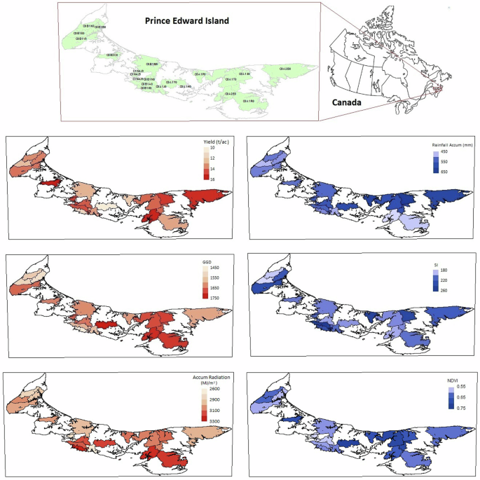
Map of PEI with selected postal codes with available data, and selected inputs averaged over years by postal code. Figure created using ArcGIS.
Local climate data (see Supplementary Table S1 for complete list) were meticulously collected from regional meteorological stations via Environment and Climate Change Canada, supplemented with sCAN (NASA Power) to ensure comprehensive coverage and continuity throughout the growing season47,48. Each farmer’s field location, identified by latitude and longitude, was matched to the nearest weather station within a 5 km radius. This comprehensive approach allowed us to capture the intricate details of the agroclimatic conditions influencing crop yields in PEI.This dual-source approach guarantees that our climate data are not only extensive but also accurately represent the microclimatic variations across different parts of the island. Our agroclimatic indices include effective growing degree days (GDD) above a base temperature of 5 °C, available soil water presented as the percentage of water holding capacity (PrcnAWHC), and the crop water stress index (SI), described in Eq. (3). Our dataset also includes average minimum and maximum temperatures, accumulated rainfall, average wind speed, and average rainfall with a 7-day lag.
Soil composition and health data were sourced from the Canadian Soil Information Service (CanSIS)49. We focused on characteristics crucial to potato cultivation, particularly in the top four soil layers (to a depth of approximately 44 cm), as this is where the plant extracts nutrients and water from the soil50. This aggregation closely reflects the root zone environment of russet potatoes. To assess plant health and growth dynamics across various stages of the potato growth cycle, satellite-derived NDVI measurements were obtained from the NOAA’s Global Vegetation Index (GVI) dataset. Weekly NDVI composites were acquired from May to the end of October, spanning from 2000 to 2016, with a spatial resolution of 1 km. These composites were quality controlled to remove cloud-affected pixels and averaged to represent each postal code area. This spatially detailed view of vegetation health was used as a critical input for predicting agricultural productivity51.
The evapotranspiration used in water balance for each field was calculated using the Penman-Monteith equation52, as shown in Eqs. (1) and (2), which has been adjusted for PEI conditions to account for local radiation, humidity, wind speed, and temperature53,54. We assumed that fields were at maximum water-holding capacity at the start of the season due to snowmelt and early precipitation. Subsequently, we calculated the percentage of water-holding capacity based on ongoing rainfall and the evapotranspiration of the plants. Evapotranspiration, a key factor in water balance, was computed using temperature data with a base temperature of 5 °C for growing degree days, ensuring accurate reflection of potato growth conditions.
Weekly NDVI composites were obtained from the MODIS platform, covering the growing season from May to the end of October (Julian Weeks 18–43), with a spatial resolution of 1 km across PEI’s agricultural regions. The data underwent quality control to remove cloud-affected pixels before generating the weekly composites14. To focus on potato-growing areas, a crop mask was applied to filter out non-agricultural and non-target pixels. The weekly NDVI values were averaged at the postal code level, and three-week running means were calculated and used as potential predictors. Additionally, the maximum and minimum NDVI values for each postal code during the growing season were extracted and included as potential predictors for yield modeling23.
To capture temporal variability, we divided the growing season into three periods: start season (SS) from May to June, mid-season (MS) from July to August, and late season (LS) from September to October. The growing season refers to the period when potatoes can grow in PEI, as the weather during these months is favorable for potato cultivation. While the exact timing of growth stages can vary each year depending on temperature and weather conditions, on average, seeding typically occurs in May and harvesting in October. The growing season was divided into these three periods based on domain knowledge of when the crop typically reaches different growth stages, with the early season generally covering the vegetative growth stage and the late season focusing on tuber maturation and harvest preparation. For each of these periods, we recorded maximum and minimum temperatures, rainfall, and soil indicators. The crop water stress index and percentage of water holding capacity were also categorized by these seasonal periods23. The indices were aggregated and averaged monthly to align with the growing season. We also calculated the standard deviations of daily precipitation, GDD, and SI for each month as potential predictors. The percentage of AWHC was computed by averaging these values for the entire season and then dividing them according to the three defined periods. For each period, we computed indicators such as the mean and the 7-day lag, which involved calculating a rolling window average to smooth short-term fluctuations and highlight longer-term trends.
Preprocessing and feature engineering
The data preprocessing began with scaling to minimize the influence of extreme values in variables like rainfall and temperature, ensuring stable and consistent data for model training. Standardization was applied to scale features like soil pH levels and NDVI measurements, ensuring that no single variable dominated due to scale differences. Feature engineering was focused on capturing temporal dynamics crucial to agricultural outputs. We crafted features to reflect the nuanced impact of seasonal climatic effects on potato growth. Rainfall data were segmented into start, middle, and late season accumulations to align with potato phenological stages, recognizing that water availability impacts tuber initiation, development, and maturation differently36. Similarly, temperature variables were segmented to account for their differing impacts on plant physiology, such as the influence of maximum and minimum temperatures on photosynthesis and metabolic rates. To provide a comprehensive view of the climatic conditions, we computed several derived features from the primary data. These included the mean minimum and maximum temperatures for the overall growing season, total rainfall accumulation, mean wind speed, and growing degree days above 5 °C (GDD5). Additionally, we calculated weekly lagged rainfall sums to capture short-term water availability dynamics. The growing season was divided into three critical periods: start, middle, and late. The start season encompassed May and early June, the middle season included June, July, and August, and the late season covered September and October. For each of these periods, specific metrics were computed, including temperature metrics that included the average maximum and minimum temperatures for each period, reflecting their different impacts on plant physiology37.
We employ a comprehensive set of climatic and soil moisture variables to assess their impact on crop yield across various growth stages. Key to our analysis is the calculation of evapotranspiration using the FAO Penman-Monteith method53, which integrates solar radiation, air temperature, humidity, and wind speed to estimate the reference evapotranspiration (ET0). This is represented by the equation:
where Δ denotes the slope of the vapor pressure curve, Rn is the net radiation at the crop surface, γ is the psychrometric constant, Tmean,K is the mean air temperature, u2 is the wind speed, es is the saturation vapor pressure, and ea is the actual vapor pressure.
The crop-specific evapotranspiration (ETc) is then computed as a product of ET0 and a dynamically adjusted crop coefficient (Kc), which varies with the accumulated growing degree days (GDD), reflecting the crop’s development stage:
Simultaneously, soil moisture dynamics are quantified using the crop water stress index23, defined as the ratio of actual evapotranspiration (AET) to potential evapotranspiration (PET), providing a direct measure of water stress experienced by the crop:
This index is critical for identifying periods of water deficiency which could impact crop health and yield. Additionally, the available water content, expressed as a percentage of the soil’s water holding the capacity (PctAWHC), is calculated to assess the soil’s ability to retain moisture, which is pivotal for irrigation management and drought assessment:
Where available soil water was computes as:
These metrics, derived from aggregated climate data by postal code and year, provide a detailed understanding of the interactions between climate variability, soil moisture status, and crop water needs. By integrating these variables into predictive models, we aim to enhance the accuracy of potato yield predictions, taking into account the complex interplay of environmental factors that influence agricultural productivity.
Research has shown that MODIS NDVI outperforms other indices, such as the National Oceanographic and Atmospheric Administration’s (NOAA) Advanced Very High Resolution Radiometer (AVHRR) NDVI, in capturing seasonal changes in vegetation, known as phenology55,56. MODIS-based NDVI is particularly effective in accurately reflecting seasonal variations across different biomes, making it highly reliable for monitoring crop growth stages and assessing plant health22. This high level of accuracy and reliability makes MODIS NDVI a valuable tool for improving the precision of our yield forecasting models. To derive NDVI features, we utilized several computational techniques to capture critical aspects of vegetation health and growth dynamics throughout the growing season. Starting with weekly NDVI data, we filtered for relevant weeks within the growing season, spanning from week 18 to week 42, to focus on the most agriculturally significant period. Missing NDVI values within each postal code and year group were handled using linear interpolation, followed by forward and backward filling to ensure continuity14. We engineered a suite of features to encapsulate the temporal patterns and variability in NDVI values. The peak NDVI feature, representing the maximum observed NDVI value within the growing season, and the corresponding time to peak NDVI were calculated to identify the period of maximum vegetative vigor. Intra-annual trends for NDVI metrics, such as minimum, maximum, and range, were computed using linear regression to capture the growth trajectory over time. To account for periodic patterns in vegetation growth, we added Fourier features by generating sine and cosine transformations of the day of the year (DOY), considering harmonics up to the third order57. This approach allowed us to model seasonal cycles effectively. Additionally, we incorporated rolling average features for NDVI metrics using a three-week window, smoothing short-term fluctuations and providing a more stable representation of vegetative health. The aggregated NDVI data were summarized by calculating mean values for NDVI metrics (Min, Max, Range), as well as their rolling averages and Fourier components, for each postal code and year. The resulting features included mean NDVI metrics, rolling averages, Fourier components, peak NDVI, time to peak NDVI, and intra-annual trends for each NDVI metric. This comprehensive set of NDVI-derived features enabled our models to capture complex patterns in vegetation growth and health, contributing significantly to the accuracy of our potato yield predictions.
Feature selection was a critical component of our preprocessing pipeline to optimize model performance. Initially, all 58 features were included for evaluation, but the number of features used in model training was later reduced using the Select K Best method. This feature selection process was embedded into our modeling pipelines and applied after scaling and other preprocessing steps. The Select K Best method was used with a range of K values (e.g. 20–58), and we utilized a Grid Search algorithm to tune K along with model hyperparameters. We implemented two primary preprocessing techniques:
-
1.
Polynomial Transformations
-
Normalization using StandardScaler to standardize the data.
-
Polynomial feature generation using PolynomialFeatures.
-
Feature selection with SelectKBest.
-
-
2.
Power Transformations
-
Robust scaling using RobustScaler to handle outliers.
-
PowerTransformer for Gaussian-like distribution transformation.
-
Feature selection with SelectKBest.
-
Model selection and training
We employed a machine learning strategy involving various predictive models, fine-tuned through comprehensive parameter optimization. These models were grouped into three categories: linear models, tree-based models, and ensemble methods. Linear models, such as Lasso and Ridge regression, were chosen for their simplicity and ability to manage overfitting through regularization. Tree-based models, including Decision Tree and Random Forest, were selected for their capacity to handle non-linear relationships and capture complex feature interactions, with Random Forest leveraging multiple decision trees to improve stability. Ensemble methods, such as AdaBoost and Gradient Boosting, were used for their strength in combining multiple models to enhance prediction accuracy. Techniques like voting, stacking, and bagging were applied to balance the insights of different algorithms, improving overall performance32. To further refine predictions, models like Decision Tree, AdaBoost, Random Forest, Gradient Boosting and Lasso Regression were combined using stacking, voting, and bagging techniques. Two distinct preprocessing pipelines were employed: the first created polynomial features after normalizing the data with Standard Scaler and selecting the top features; the second used robust scaling to handle outliers, followed by feature selection and transforming features into a Gaussian-like distribution using the Yeo-Johnson method33,34. Figure 5 shows the pipeline applied to our dataset for yield prediction, including data preprocessing, model training, hyperparameter optimization, model selection, evaluation, and final results.
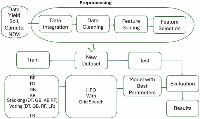
Data preprocessing, model training with multiple algorithms, hyperparameter optimization (HPO), testing, and evaluation. Figure created using PowerPoint.
To prevent data leakage, we employed cross-validation27. This method respects the temporal order of data by training models on past data and testing them on future data, thereby maintaining the chronological sequence and preventing the model from gaining undue information from future data points. This approach is crucial for ensuring that the model’s predictive performance is evaluated in a realistic setting, simulating how it would perform in actual deployment. Parameter tuning and validation were integral to our methodology. Detailed parameter tuning was conducted using Grid Search, which systematically explores combinations of parameters to identify the optimal configurations for each model58. For instance, the AdaBoost model was tuned with parameters such as the number of estimators, learning rates, and loss functions, while Bayesian Ridge and Decision Tree models had their respective parameters systematically adjusted. The Grid Search optimization algorithm iterates through the specified parameter grid and evaluates each combination using cross-validation to determine the best set of parameters. This process involved setting up a 5-fold cross-validation scheme, ensuring that each model was rigorously evaluated across different subsets of the data. This approach helps mitigate the risk of overfitting and provides a robust measure of model performance. All models, including the ensemble techniques, were trained with each of these preprocessing pipelines and optimized using a parameter grid through Grid Search optimization and cross-validation32,59. This approach ensured that we could identify the best-performing model configurations under different data transformations. The use of distinct preprocessing techniques allowed us to capture a wide range of feature interactions and distributions, enhancing the robustness and generalizability of our predictive models. By rigorously optimizing parameters and validating models across various data transformations, we ensured the reliability and accuracy of our yield predictions.
To interpret our models effectively and understand the influence of each feature on predictive outcomes, we employed two key techniques: impurity-based feature importance and SHapley Additive exPlanations (SHAP) values40,60. Impurity-based feature importance was used to identify key factors, where higher-ranked features are likely to directly or indirectly influence yield or interact significantly with other variables. SHAP values provided a per-sample breakdown of feature importance, allowing us to analyze the contributions of each feature to the model’s predictions. By aggregating SHAP values and feature importance scores across all model predictions and preprocessing pipelines, we gained a comprehensive overview of the most influential factors in predicting yield. This approach facilitated a deeper understanding of the underlying patterns in the data and the model’s decision-making process. These interpretative tools, combined with robust preprocessing and extensive parameter tuning, enabled us to develop highly accurate predictive models for potato yields in Prince Edward Island, providing valuable insights for strategic agricultural planning and management.

Responses