Advancing extrapolative predictions of material properties through learning to learn using extrapolative episodic training
Introduction
In recent years, machine-learning algorithms have demonstrated the potential to accelerate the discovery of new materials in diverse material systems such as polymers1, inorganic compounds2,3, alloys4, catalysts5,6, and aperiodic materials7,8,9. Central to this advancement is a rapidly computable property predictor obtained through machine learning that represents the compositional and structural features of any given material in the vector form and learns the mathematical mapping of these vectorized materials to their physicochemical properties. By employing such a property predictor with millions or even billions of candidate materials, novel materials with tailored properties can be effectively identified by navigating an extensive search space.
The most significant challenge in data-driven materials research is the scarcity of data resources10,11,12. In most research tasks, ensuring a sufficient quantity and diversity of data remains challenging. Furthermore, the ultimate goal of materials science is to discover “innovative” materials from an unexplored material space. However, machine-learning predictors are generally interpolative and their predictability is limited to the neighboring domain of the training data. Even large language models, which are currently revolutionizing various fields, are essentially memorization learners that make interpolative predictions based on a considerable amount of data13. Therefore, establishing fundamental methodologies for extrapolative predictions is an unsolved challenge not only in materials science but also in the next generation of artificial intelligence technologies14,15,16.
Research on extrapolative machine learning has progressed through various frameworks, including domain generalization17,18, transfer-learning19, domain adaptation20,21, meta-learning22, and multitask learning23, all of which are closely interrelated. These methodologies aim to overcome the challenge of limited data by integrating heterogeneous datasets with various generative processes in the source and target domains. Wu et al. (2019) employed transfer-learning to successfully discover three new amorphous polymers with notably high thermal conductivities1. Owing to the limited availability of thermal conductivity data for only 28 amorphous polymers in the target domain, they constructed a transferred thermal conductivity predictor by refining a collection of source models pretrained on other related properties, such as the glass transition temperature, specific heat, and viscosity, for which a comprehensive dataset existed. Remarkably, the dataset for the target task lacked similar instances for the three synthesized polymers. Nevertheless, the transferred model exhibited an extrapolative generalization performance owing to the presence of relevant cases in the source datasets. In materials research, several instances of using transfer-learning to successfully acquire extrapolative capabilities have been reported24,25. In the growing fields of artificial intelligence, such as computer vision and natural language processing, research on domain generalization is considerably more active than in materials science17,18,26,27. For example, in domain generalization, numerous sets of data from different domains, called episodes, are generated from an entire dataset, and the model repeatedly undergoes domain adaptation28,29. During repetitive training, the resulting model often acquires domain-invariant feature representations, thus achieving generalization for unseen domains. For example, a set of episodes can be generated by manipulating an original image by varying its appearance, brightness, and background. In materials research, different material classes, such as polyesters and cellulose, can correspond to different domains. However, it is uncertain whether generic domain generalization methodologies are effective for material-property prediction tasks. It is intuitively plausible that a domain-invariant representor or predictor exists across synthetically manipulated images. However, it is not obvious whether such invariance exists in different material systems.
In this study, we leveraged an attention-based architecture originally designed for few-shot learning, called the matching neural network (MNN)30, to learn the learning method for obtaining extrapolative predictors. We employed a meta-learning algorithm30,31,32,33,34, commonly known as “learning to learn,” to impart extrapolative prediction capabilities to the MNNs. Numerous episodes were generated from a given dataset ({{{mathcal{D}}}}), each comprising a training set ({{{mathcal{S}}}}) and test set ({{{mathcal{Q}}}}) containing instances outside the training domain ({{{mathcal{S}}}}). The objective was to learn a generic model (y=f(x,{{{mathcal{S}}}})) representing the mapping from material x to property y, where (x, y) belong to domain ({{{mathcal{Q}}}}). MNNs have a distinctive feature in that they explicitly include the training dataset ({{{mathcal{S}}}}) as an input variable, and instances of the input-output pair (x, y) are assumed to follow a distribution different from that of ({{{mathcal{S}}}}). Unlike other domain adaptation methods, MNNs explicitly describe the model (y=f(x,{{{mathcal{S}}}})) to predict y from x in an unseen domain for a given training dataset ({{{mathcal{S}}}}).
The following sections demonstrate how extrapolatively trained predictors acquire extrapolative capabilities through two property prediction tasks for polymeric materials and hybrid organic–inorganic perovskite compounds. For a given dataset, we can generate a set of episodes for extrapolative learning with flexible quantity and quality. This is considered a type of self-supervised learning. As elucidated later, the conditions for generating episode sets, such as the overall data and ({{{mathcal{S}}}}) sizes in the training and inference phases, significantly influence the generalization performance. Through various numerical experiments, we provide guidelines for appropriately configuring these parameters. Moreover, we used the extrapolatively trained predictor as a pretrained model for downstream tasks, adapting it to the target domain using data from an extrapolative domain of the material space. This predictor demonstrates higher transferability, requiring fewer training instances for downstream extrapolative prediction tasks compared to conventionally trained models.
Results
Methods outline
A conventional machine-learning-based predictor describes the relationship between input x and output y as y = fϕ(x). After training the model, the parameter ϕ is entered as an implicit function of the training dataset ({{{mathcal{S}}}}) as (y={f}_{phi ({{{mathcal{S}}}})}(x)). In contrast, the meta-learner (y={f}_{phi }(x,{{{mathcal{S}}}})) takes both the input–output variables (x, y) and the training dataset ({{{mathcal{S}}}}={{x}_{i},{y}_{i}| i=1,ldots ,m}) comprising m instances as the argument. In the context of meta-learning, ({{{mathcal{S}}}}) is referred to as a support set. From a given dataset ({{{mathcal{D}}}}={{x}_{i},{y}_{i}| i=1,ldots ,d}), a collection of n training instances, ({{{mathcal{T}}}}={{x}_{i},{y}_{i},{{{{mathcal{S}}}}}_{i}| i=1,ldots ,n}), referred to as episodes, is constructed to train the meta-learner. In this scenario, for each episode (xi, yi) and ({{{{mathcal{S}}}}}_{i}), tuples in an extrapolative relationship can be arbitrarily selected. For instance, (xi, yi) represents the physical property yi of a cellulose derivative xi, whereas ({{{{mathcal{S}}}}}_{i}) represents a dataset from other polymer classes, such as conventional plastic resins. Alternatively, (xi, yi) can correspond to a compound containing element species that do not exist in the training compounds comprising ({{{{mathcal{S}}}}}_{i}). An essential aspect is that such extrapolative episodes can be arbitrarily generated from any given dataset. This learning scheme is denoted as extrapolative episodic training (E2T) (Fig. 1).
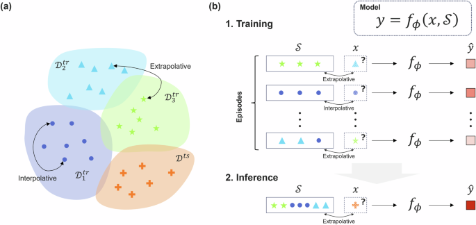
a Data partitioning to generate extrapolative training sets. b Training and inference procedures. E2T with MNNs involves the generation of numerous episodes from a given dataset, comprising a support set (({{{mathcal{S}}}})) and an input-output pair (x, y). By including many ({{{mathcal{S}}}}) and (x, y) with extrapolative relationships into the episode set, the trained MNN learns the general form (y=f(x,{{{mathcal{S}}}})) for extrapolatively predicting from x to y for any given ({{{mathcal{S}}}}).
This study focuses on a real-valued output (yin {mathbb{R}}) that represents a physical property. The proposed model is an attention-based neural network that associates the input and output variables as follows:
Output y is computed by considering the weighted sum of yi within the support set ({{{mathcal{S}}}}) using weight (a({phi }_{x},{phi }_{{x}_{i}})). The second equation is represented in the vector form by ({{{{bf{y}}}}}^{top }=({y}_{1},ldots ,{y}_{m})in {{mathbb{R}}}^{m}) and ({{{bf{a}}}}{(x)}^{top } = (a({phi }_{x},{phi }_{{x}_{1}}),ldots ,a({phi }_{x},{phi }_{{x}_{m}}))in {{mathbb{R}}}^{m}). Attention (a({phi }_{x},{phi }_{{x}_{i}})) evaluates the similarity between inputs x and xi in the support set through neural embedding ϕ.
In this study, we employed the following attention mechanism that resembles a kernel ridge regressor:
where ({{{{bf{y}}}}}^{top }=(1,{y}_{1},ldots ,{y}_{m})in {{mathbb{R}}}^{m+1}), ({{{bf{g}}}}{({phi }_{x})}^{top }=(1,k({phi }_{x},{phi }_{{x}_{1}}),ldots , k({phi }_{x},{phi }_{{x}_{m}}))in {{mathbb{R}}}^{m+1}), and Gϕ is a (m + 1) × (m + 1) Gram matrix of positive definite kernels (k({phi }_{{x}_{i}},{phi }_{{x}_{j}})) and is defined as
In Eq. (2), I is a (m + 1) × (m + 1) identity matrix and (lambda in {mathbb{R}}) is a controllable smoothing parameter. Note that a constant of 1 is included in y, g(ϕx), and the first row and column of Gϕ to introduce an intercept term into the regressor. Here, ({{{bf{a}}}}{({phi }_{x})}^{top }={{{bf{g}}}}{({phi }_{x})}^{top }{({G}_{phi }+lambda I)}^{-1}) according to Eq. (1). Bertinetto et al.35 proposed this model as a differentiable closed-form solver in the context of few-shot learning by using model-agnostic meta-learning (MAML)34 to obtain a meta-learner that is rapidly adaptable to various tasks.
E2T learning is formulated as ℓ2 loss minimization as follows:
In the two case studies employed in this study, we modeled the feature embedding ϕ using neural networks (more details are provided in the Methods section).
The method for generating episodes involved different strategies for each case study. Intuitively, it is natural to include both extrapolative and interpolative episodes in a dataset, rather than relying solely on extrapolative episodes. However, the mixing ratio of extrapolative to interpolative episodes influences the learning performance. It is important to note that the size of ({{{mathcal{S}}}}) can be arbitrarily adjusted. Particularly, the size of ({{{mathcal{S}}}}) can differ between the training and inference phases, and increasing its size increases the computational burden, particularly when calculating the inverse matrix in Eq. (2). To mitigate the computational cost, a randomly sampled ({{{mathcal{S}}}}) should be employed. However, the optimal size of ({{{mathcal{S}}}}) for the training and inference phases must be determined. To address this issue, we conducted various numerical experiments during the two case studies.
Experimental results
The learning behavior and potential mechanisms of E2T were experimentally investigated. This section presents the performance evaluation experiments that focused on extrapolative prediction tasks for amorphous polymers and hybrid organic–inorganic perovskites.
Prediction of polymer property across different classes
E2T was applied to a dataset of polymer properties calculated using the RadonPy software36 that automates the process of all-atom classical molecular dynamics (MD) simulations for various polymeric properties, including specific heat at constant pressure (Cp) and refractive index. The dataset included 69,480 amorphous polymers classified into 20 polymer classes, denoted by p01–p16 and p18–p21 where p17 is a missing class, such as polyimide, polyesters, and polystyrene, based on the chemical structures of their repeating units (Supplementary Table S1). Visualization of the chemical space using the uniform manifold approximation and projection (UMAP) method37 showed that these polymer classes were structurally distinct (Supplementary Fig. S1), indicating that the prediction tasks across different polymer classes were extrapolative. Here, it should be noted that the training and test data distributions are not completely separate.
To evaluate the prediction performance for an unseen polymer class, the following process was implemented: (1) a model was trained using randomly selected samples from 19 of the 20 polymer classes and (2) its generalizability was assessed using data from the remaining polymer class. Two tasks were performed to predict Cp and the refractive index. The chemical structure of a polymer repeating unit was encoded through Morgan fingerprinting38,39 into a 2048-dimensional descriptor vector, which served as the input for a three-layer fully connected neural network (FCNN) employed as the embedding function ϕ of MNN. As a baseline, a conventional FCNN with three hidden layers, which had an architecture similar to the embedding function of the MNN, was subjected to ordinary supervised learning.
We assessed the scalability of the model’s generalization capability with respect to the sample size of the training set ({{{mathcal{D}}}}) and support set ({{{mathcal{S}}}}). In each step of E2T, a training instance on (x, y) was sampled from a randomly selected polymer class, whereas the support set ({{{mathcal{S}}}}) was entirely sampled from the 19 polymer classes, including interpolative and extrapolative episodes. Throughout the training process, the size of the support set was fixed at m = 30, whereas during the inference phase, the overall training dataset, ({{{mathcal{D}}}}), was set to ({{{mathcal{S}}}}). The hyperparameter λ was set to 0.1, and its influence on the resulting extrapolative prediction performance was investigated through a sensitivity analysis, as described later. These experiments were independently repeated 10 times to calculate the prediction accuracy and its variability. Further details are provided in the Methods section.
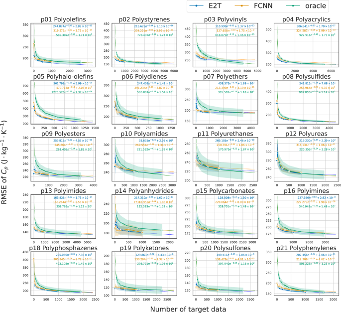
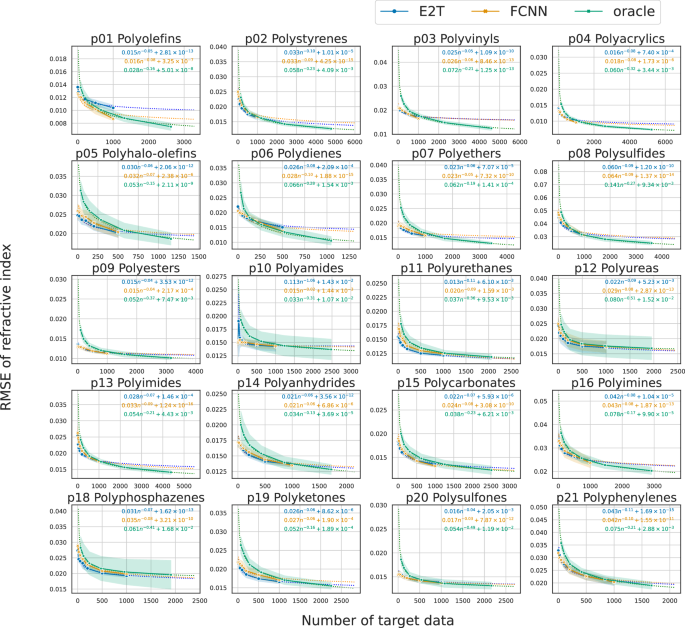
Figures 2 and 3 present the predictive performance for each of the 20 unseen polymer classes, exhibiting almost monotonical improvements with the increasing size of the training set ({{{mathcal{D}}}}). For each task in Cp (Fig. 2) or refractive index (Fig. 3), E2T consistently and significantly outperformed ordinary supervised learning with FCNN for most polymer classes across varying sizes of ({{{mathcal{D}}}}) in the range [950, 38000]. The generalizability of E2T was scaled according to a power law with an increasing training set size of approximately the same order of magnitude as that of ordinary supervised learning. In particular, there were no cases wherein E2T significantly underperformed ordinary learning. However, it did not show notable improvements in the Cp prediction for several polymer classes, such as polyimides (p13), polyanhydrides (p14), and polyphosphazenes (p18). Unfortunately, the underlying cause for this could not be identified. The distributional features of the property values for each polymer class, as presented in Supplementary Fig. S2, did not exhibit any notable patterns associated with the observed extrapolative behaviors. Additionally, structural visualization through UMAP projections, as shown in Supplementary Fig. S1, do not reveal any structural uniqueness in these polymer classes. For example, p14 and p18 exhibited no significant improvements in the Cp prediction task. However, E2T demonstrated a substantial improvement over ordinary learning for refractive index prediction on p14 and p18. This observation suggests that the potential gain in extrapolative prediction arises does not only from cross-domain similarities or differences in molecular structures, but also from the potential transferability determined by the presence or absence of a shared functional relationship (y=f(x,{{{mathcal{S}}}})) across domains.
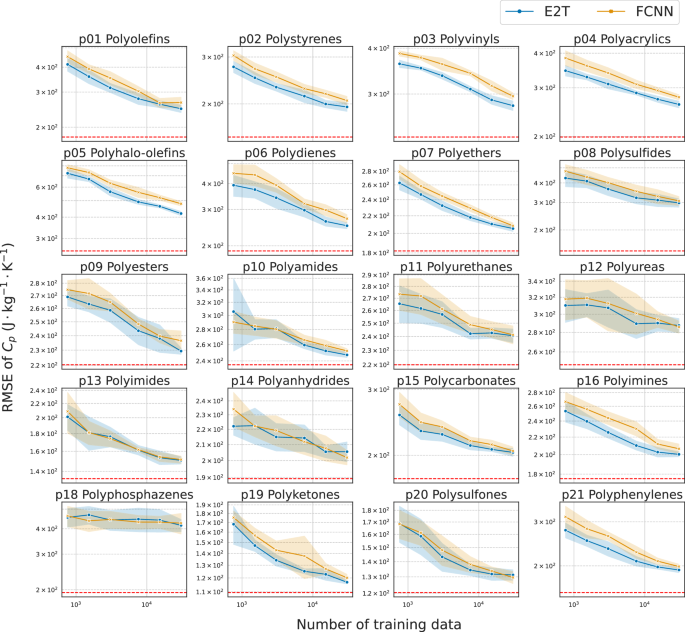
The RMSEs of MNNs trained with E2T and conventional FCNNs are indicated in blue and orange, respectively. The red dashed lines denote the generalization performance of oracle predictors derived from conventional domain-inclusive learning, which utilized data from all polymer classes. The shaded areas indicate the standard deviations.
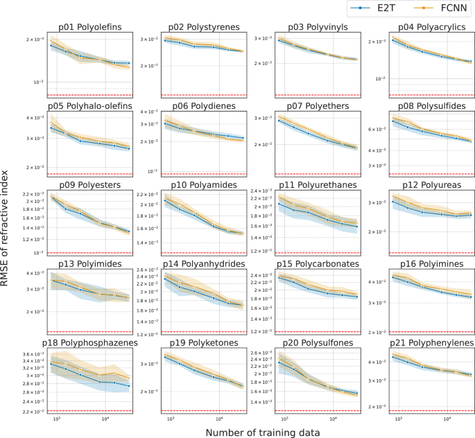
The RMSEs of MNNs trained with E2T and conventional FCNNs are indicated in blue and orange, respectively. The red dashed lines denote the generalization performance of oracle predictors derived from conventional domain-inclusive learning, which utilized data from all polymer classes. The shaded areas indicate the standard deviations.
The gain of E2T over ordinary supervised learning was substantially smaller for refractive index than for Cp (Figs. 2 and 3). This is likely because the refractive index prediction task is less challenging, allowing ordinary supervised learning to achieve high accuracy. Supplementary Figure S3 shows the prediction results for refractive index and Cp obtained from ordinary supervised learning: R2 reached 0.937 ± 0.003 for the refractive index with only 3435 samples.
Furthermore, we investigated the generalization performance of the FCNN trained on approximately 55,580 randomly selected samples from all polymer classes containing the target domain. Hereafter, we refer to these predictors as “oracles.” As shown in Figs. 2 and 3 with red dashed lines, for most polymer classes, the extrapolative capability of E2T could not match that of the interpolative prediction of the oracle predictors. This suggests that although E2T enhanced the extrapolative performance, it does not impart a fundamental extrapolation capability. However, as demonstrated later, E2T can attain a generalization performance similar to or significantly better than that of the oracle predictors with considerably fewer training samples when fine-tuned to the target domain. This implies that extrapolatively trained models can rapidly adapt to a target domain using a small dataset.
Bandgap prediction of perovskite compounds
To verify the generalizability of E2T, we conducted another experiment using a hybrid organic–inorganic perovskite (HOIP) dataset40,41, which includes 1345 perovskite structures and their properties, including bandgaps, as calculated through the density functional theory. Each perovskite comprises a combination of organic/inorganic cations and an inorganic anion. The inorganic elements in the cations are germanium (Ge), tin (Sn), and lead (Pb), whereas the element in the anion is given by fluorine (F), chlorine (Cl), bromine (Br), or iodine (I). Na et al.42,43 demonstrated state-of-the-art extrapolation performance using an automated nonlinearity encoder (ANE) on the HOIP dataset. ANE aims to enhance the extrapolative prediction performance by utilizing an embedding function of input crystal structures that are pretrained through self-supervised learning based on deep metric learning. Specifically, the embedding function was trained by minimizing the Wasserstein distance between two given instances in the embedding and property spaces, followed by ordinary supervised learning to predict the physical properties using the embedded crystal structures. They considered two tasks mimicking real-world scenarios for exploring novel solar materials: excluding perovskites containing both (1) Ge and F and (2) Pb and I from the training dataset. We refer to these tasks as “HOIP-GeF” and “HOIP-PbI.” As shown in Supplementary Figs. S4 and S5, the distributions of the training and test sets in both tasks were extrapolatively related in both the structure and property spaces. In particular, the bandgap distributions of HOIP-GeF and HOIP-PbI were significantly biased toward higher and lower tails, respectively. It should be noted, however, that the training and test data distributions are not perfectly distinct.
We performed numerical experiments using the same setting as that employed by Na et al.42,43. The HOIP dataset was divided into 12 groups based on the combinations of four anions and three cations. For creating a training episode, we excluded all samples with Ge and F or those with Pb and I and randomly selected 50 instances of (x, y) from one group while drawing ({{{mathcal{S}}}}) of size 50 from the 10 remaining groups. In total, 1248 or 1228 training samples were drawn from the overall data, respectively. Further experimental details are provided in the Methods section. During the inference phase, the entire training dataset ({{{mathcal{D}}}}) was assigned to ({{{mathcal{S}}}}).
We compared the performance of E2T with that of ANE and conventional supervised learning. ANE and E2T were modeled using an embedding function, followed by a regression header for computing the bandgap as the output. To embed the input crystal structures, a message-passing neural network (MPNN)44, which is a graph neural network, was used for ANE and E2T. As for the models used in the header part, ANE and E2T employed FCNN and kernel ridge regressor, respectively. Moreover, “MPNN-Linear” with a linearly modeled top layer and “MPNN-FCNN” were used as additional baselines.
The extrapolative prediction accuracies are summarized in Table 1. Similar to the polymer-property prediction tasks, the extrapolative prediction performance of E2T substantially surpassed that of conventional learning models (MPNN-Linear and MPNN-FCNN) for both HOIP-GeF and HOIP-PbI, and significantly exceeded that of ANE. Interestingly, although E2T did not obtain the baseline prediction performance of an oracle predictor with an ordinary FCNN trained on the entire dataset, including instances from the target domain, it achieved a remarkably close performance to it (Table 1). For example, the coefficients of determination (R2) of E2T and the oracle were 0.605 ± 0.057 and 0.766 ± 0.113 for HOIP-PbI, respectively, whereas R2 of ANE was 0.510 ± 0.108, which was similar to the results for HOIP-GeF, indicating that E2T acquired an outstanding extrapolative prediction mechanism.
We investigated the prediction performance of E2T in the interpolative domain by training the MNN using only extrapolative episodes sampled from the 11 groups, excluding the target domain, following the procedure described above. As a baseline, MPNN-Linear was trained on a dataset randomly sampled from the same 11 groups using conventional supervised learning. A test dataset was constructed by randomly selecting 20% of the dataset from the 11 groups to assess the interpolative prediction performance. For each of HOIP-GeF and HOIP-PbI, five independent trials were conducted to examine differences in average performance. As shown in Supplementary Table S2, the predictive performance of E2T in the interpolative domain was comparable to that of the baseline. This result suggests that prediction performance in the interpolative domain can be maintained even when the model is trained with extrapolative episodes.
In the episodic training framework, several hyperparameters, such as the size of the support set, must be adjusted. We conducted an ablation study using the HOIP dataset to investigate the influence of the training and inference support sizes, (leftvert {{{{mathcal{S}}}}}_{{{{rm{train}}}}}rightvert) and (leftvert {{{{mathcal{S}}}}}_{{{{rm{infer}}}}}rightvert), and the smoothing parameter λ for the ridge regressor head on the E2T performance.
As shown in Fig. 4a, the generalization performance tended to improve with an increase in the training support size (leftvert {{{{mathcal{S}}}}}_{{{{rm{train}}}}}rightvert); however, the scaling behaviors were unclear. Particularly, in the HOIP-GeF task with the optimal support size λ = 10 exhibiting the best performance among the trials, the generalization performance did not change monotonically with an increasing (leftvert {{{{mathcal{S}}}}}_{{{{rm{train}}}}}rightvert). In summary, it is appropriate to maintain a relatively small training support set while appropriately controlling the λ value.
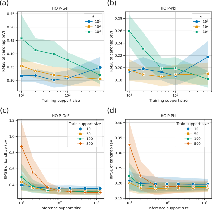
a, b RMSE variations according to varying training support sizes with the inference support size fixed at 1248 (a) and 1228 (b). c, d RMSE variations according to varying the inference support size at λ = 100. In (a, b), the colored lines indicate different smoothing parameters λ, whereas in (c, d), they represent different training support sizes. The shaded areas indicate the standard deviations.
By contrast, as shown in Fig. 4b, the generalization performance scaled monotonically with an increase in the inference support size (leftvert {{{{mathcal{S}}}}}_{{{{rm{infer}}}}}rightvert). However, the decay of the generalization performance nearly halted at approximately (leftvert {{{{mathcal{S}}}}}_{{{{rm{infer}}}}}rightvert approx 1{0}^{2}), regardless of the training support set size. Thus, the results of this test led to the conclusion that setting (leftvert {{{{mathcal{S}}}}}_{{{{rm{infer}}}}}rightvert approx 1{0}^{3}) is adequate for achieving satisfactory accuracy. In summary, it is preferable to use a large support set for inference, while ensuring an appropriate value for λ. In practice, (leftvert {{{{mathcal{S}}}}}_{{{{rm{infer}}}}}rightvert) should be sufficiently large relative to (leftvert {{{{mathcal{S}}}}}_{{{{rm{train}}}}}rightvert) under the constraint of the computational cost.
Fine-tuning to extrapolative domains
Thus far, we focused on scenarios wherein no data were available during episodic training for the target domain. Now, we focus on scenarios wherein a limited amount of data is available in the target domain; such scenarios are common in practical materials development. In such cases, leveraging data from a related source domain via transfer learning including fine-tuning is a pragmatic approach1,24. Moreover, meta-learning methods have proven effective in materials science, such as toxicity prediction45,46,47 and perovskite design48. Inspired by these studies, we adapted a pretrained meta-learner to the data from the target domain via fine-tuning, as detailed in the Methods section. The results of applying the proposed methodology to the two distinct problem settings are presented below.
Fine-tuning was performed on the RadonPy dataset. In this experiment, a pretrained E2T model with a source data size of 38,000 was fine-tuned on data from the target domain corresponding to a particular polymer class. To fine-tune a pretrained E2T, episodes (({x}_{i},{y}_{i},{{{{mathcal{S}}}}}_{i})) were randomly sampled from all data containing the polymer class of the target domain to modify the entire network. The pretrained FCNNs underwent fine-tuning across all layers of their respective networks using data from the target polymer class.
As shown in Figs. 5 and 6, the loss decreased almost monotonically as the data size in a target domain increased for E2T and FCNN. The differences between E2T and FCNN are evident in that E2T outperforms FCNN in most cases for Cp prediction, implying the superiority of E2T over ordinary supervised learning, even in fine-tuned scenarios. In particular, E2T scaled with no order-level differences but maintained constant gains as the trained data increased. Additionally, as observed with the pretrained models, the improvement of E2T over ordinary supervised learning is smaller for refractive index than for Cp, likely because predicting refractive index is easier, allowing ordinary supervised learning to achieve high accuracy (Supplementary Fig. S3).
The E2T results are depicted in blue, whereas the FCNN results are presented in orange. The scaling behavior of oracle is depicted in green. Each panel represents a different polymer class. The y-axis represents the RMSE with the standard deviation. The x-axis indicates the data size in each polymer class. Shaded areas highlight the standard deviations.
Here, a quantitative performance comparison is presented, including the oracle predictor trained on the entire dataset containing target domain samples. Figures 5 and 6 illustrate the scaling behavior of the baseline performance of the oracle relative to increasing data size in each polymer class. The E2T and fine-tuned FCNN models exhibited a downward convex pattern compared to the scaling curves of the oracle predictor, with stronger convexity indicating better domain adaptation. To quantitatively assess cross-domain transferability, we estimated a power-law function Bk(n) = Dn−α + C based on the observed scaling behavior of each algorithm k, where α represents the decay rate, C the achievable performance limit, and n the sample size per polymer class. Using the estimated lower area (int_{0}^{1000}{B}_{k}(n){{{rm{d}}}}n), the transferability was compared across E2T, fine-tuned FCNN, and oracle (Supplementary Table S3). The E2T fine-tuning model outperformed the oracle predictor in 20 and 18 of the 20 polymer classes for the Cp and refractive index prediction tasks, respectively. Furthermore, E2T outperformed the fine-tuned FCNN predictor for Cp and refractive index in 17 and 16 out of the 20 polymer classes, respectively. Few instances were observed where the performance of E2T was significantly lower than that of the oracle and fine-tuned FCNN. The smaller gain in refractive index prediction corresponds with the lower task difficulty, as previously noted.
The E2T results are depicted in blue, whereas the FCNN results are presented in orange. The scaling behavior of the oracle is represented in green. Each panel represents a different polymer class. The y-axis represents the RMSE with the standard deviation. The x-axis indicates the data size in each polymer class. The shaded areas represent standard deviations.
Similar experiments were conducted on the HOIP dataset, where MNNs pretrained with E2T on 1248 or 1228 source datasets were transferred to predict the target domains, namely HOIP-GeF and HOIP-PbI. Fine-tuning episodes were generated using samples from the source and target domains. In contrast, the pretrained MPNN-Linear model was fine-tuned on data from the target domain. The scaling behaviors are shown in Fig. 7, which highlight that E2T outperformed ordinary supervised learning, thereby supporting the conclusions of the experimental results obtained using the RadonPy dataset.
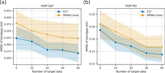
a, b The results for HOIP-GeF and HOIP-PbI, respectively. The results of E2T and MPNN-Linear are distinguished by blue and orange colors, respectively. The x-axis denotes the number of target samples used for fine-tuning, whereas the y-axis denotes the RMSE of the bandgap predictions along with the standard deviations.
Discussion
The goal of materials science is to predict material properties beyond the data distribution range. This study presented a machine-learning methodology to address this fundamental challenge. Previous approaches have relied on incorporating physical prior knowledge into models as descriptors, or employing known theories or empirical rules to model architectures through methods such as physics-informed machine learning, with the aim of achieving extrapolative predictability. In contrast, we aimed to achieve this through fully inductive reasoning without any physical insights. Specifically, we focused on the MNN architecture originally proposed for few-shot learning and used it as a meta-learner for extrapolative predictions. The meta-learner has been shown to acquire extrapolative prediction ability through numerous extrapolative tasks generated by the E2T algorithm. Although the generalization performance of the meta-learner in this study did not reach that of an oracle model learned on all datasets, including the target extrapolative domain, the significance of the extrapolative prediction performance improvement over the baseline model was substantial in most cases. Notably, there were almost no instances of significantly decreased predictive performance compared to conventional training, and the performance in the interpolation region was comparable to that of conventional training, offering a significant advantage in practical applications.
Furthermore, it was experimentally confirmed that meta-learners trained through extrapolative training can be quickly transferred to unexplored domains with a small amount of additional data, indicating the quick adaptability of learners trained to tackle challenging problems. In transfer learning research, it is theoretically and empirically demonstrated that increasing task diversity during pretraining enhances transferability to downstream tasks49,50. For instance, Mikami et al.50 showed that in vision tasks, augmenting the pretraining dataset with images of modified contrast or rotated and translated objects improves the scalability of transferred models in downstream tasks. A similar mechanism is expected to function in the fine-tuning of E2T. One of the expandable features of E2T is the flexibility in designing episode sets. For instance, although we fixed the size of the support set in this study, it is possible to include support sets of varying sizes, including extremely small data, in the training dataset to create a few-shot meta-learner. It would be intriguing to explore the predictive capabilities achieved with increased task diversity.
However, this study is just the first step in this domain, and several technical challenges and research questions remain to be addressed. The computation of MNNs requires storing past training data in memory as the support set, which limits the amount of data that can be retained and also raises privacy concerns. Additionally, as the data volume increases, the computational load of the kernel ridge regression header increases. Leveraging other meta-learning methodologies such as MAML or its derivatives could address these issues. Furthermore, various hyperparameters must be considered for designing the method of generating episode sets. Although E2T demonstrates better performance compared to conventional methods, the degree of improvement is limited, necessitating further tuning. In particular, the ratio of interpolative to extrapolative episodes in the episode set is expected to affect the generalization performance. For example, a learner that is primarily trained on extrapolative episodes may not exhibit satisfactory performance interpolative predictions. This relates to curriculum learning (easy-to-hard learning strategy)51 and hard example mining (focus on hard example)52. However, the optimal strategy remains unresolved. Furthermore, it is also intriguing to investigate whether the observed early adaptability of meta-learners to new tasks is universally valid.
Methods
Polymer property prediction
Data
In the polymer-property prediction experiments, 69,480 samples of Cp and 68,700 samples of the refractive index were used for the amorphous homopolymers. The data were generated using RadonPy36, which is a Python tool to construct a workflow for fully automated calculations of various polymeric properties using all-atom MD simulations. This dataset included 1078 samples provided by Hayashi et al. (2022)36 and those newly generated by the RadonPy consortium. Approximately 70,000 hypothetical polymers were generated using an N-gram-based polymer structure generator53 and classified into 20 polymer classes based on the classification rules established by PolyInfo54. A list of 20 polymer classes and their data sizes is presented in Supplementary Table S1.
Descriptor
The count-based Morgan fingerprint38, a type of extended connectivity fingerprint (ECFP)39, was utilized as a descriptor for the repeating unit of a homopolymer. The descriptor was calculated using RDKit55, with a radius of 3 and bit length of 2048.
Training of MNNs by E2T
The attention-based model, which resembles the kernel ridge regressor in Eq. (2), was implemented in PyTorch56. A three-layer FCNN with the rectified linear unit (ReLU) activation function was used as the embedding function ϕ to define the mapping from the 2048-dimensional descriptor to the 16-dimensional latent space. The layer structure of ϕ was configured with 2048, 128, 128, and 16 neurons, and the last 16-dimensional vector was normalized through layer normalization57. For the ridge regressor head, the smoothing parameter was set to λ = 0.1.
Data of 19 of 20 polymer classes were used for training, whereas the remaining class was used for testing to evaluate the extrapolative prediction performance of the model. To investigate the influence of the training dataset size on the generalization performance, the number of training samples was varied among (| {{{mathcal{D}}}}| in {950,1900,3800,9500,19000,38000}). The training set was generated from 19 polymer classes such that the number of samples from each class was the same. Each training set was further split into training ({{{{mathcal{D}}}}}_{{{{rm{train}}}}}) and validation ({{{{mathcal{D}}}}}_{{{{rm{val}}}}}) sets at a ratio of 80:20. In each step of E2T, a training instance on (x, y) was sampled from a randomly selected polymer class, whereas the support set ({{{mathcal{S}}}}) of size m = 30 was sampled entirely from the 19 polymer classes, including interpolative and extrapolative episodes. During the training process, the prediction performance was monitored using the validation loss.
Training was halted if no improvement was observed over 90,000 episodes. The training was performed with a dropout rate58 of 0.2 and constant learning rate of 2 × 10⁻⁴ using the Adam optimizer59. Hyperparameters were selected to stabilize the training based on a few preliminary runs. The trained model was evaluated using the data from the remaining polymer class. These experiments were repeated ten times for each condition using different random seeds.
Training of fully connected networks by ordinary supervised learning
Four-layer FCNNs configured with 2048, 128, 128, 16, and 1 neurons were implemented using PyTorch. ReLU was used as the activation function, and layer normalization was applied to the 16-dimensional hidden representation. Data from 19 of 20 polymer classes were used for training, and the remaining class was used to evaluate the performance of the extrapolative prediction. To investigate the influence of the size of the training dataset on the performance, different dataset sizes (leftvert {{{mathcal{D}}}}rightvert in {950,1900,3800,9500,19000,38000}) were sampled from the dataset in the 19 classes to ensure that the same number of samples were included from each polymer class; 20% of the training set was used for validation. Training was performed with a dropout rate of 0.2, batch size of 256, and constant learning rate of 2 × 10⁻⁴ using the Adam optimizer. Additionally, training was terminated when no improvement was observed over 50 epochs, and the trained model was evaluated using the data from the remaining polymer class. The experiment was repeated ten times for each condition using different random seeds.
Generalization performance of domain-inclusive learning
Four-layer neural networks were implemented to evaluate the generalization performance for domain-inclusive learning by using data from the entire chemical space. The entire data, including 20 polymer classes, were split into training, validation, and test sets at a ratio of 64:16:20. Using the training and validation sets, the networks were trained using the same procedure as that for training the FCNNs in the extrapolative prediction task. The trained model was evaluated on the test set for each polymer class. The experiment was repeated five times using different data splits.
Bandgap prediction of perovskite compounds
Data
The HOIP dataset40,41 contains 1345 perovskite compounds and their properties, including bandgaps, dielectric constants, and relative energies, calculated using the density functional theory. Each compound comprises an organic cation, inorganic cation, and inorganic anion. The inorganic elements comprise Ge, Sn, and Pb cations and F, Cl, Br, and I anions. In this experiment, similar to previous studies42,43, we performed two distinct tasks to assess the generalization performance of the model: (1) bandgap prediction of perovskite compounds containing Ge and F, and (2) prediction of perovskite compounds containing Pb and I. The former and latter sets exhibit extremely high and low bandgaps, respectively.
Embedding function of crystal structures
The MPNN44 was employed as the encoder for the crystal structures in all models. The MPNN architecture was designed in a manner similar to that proposed by Na and Park42, with an embedding size of 32. For more details, please refer to the following GitHub repository: https://github.com/ngs00/ane.
Training of MNNs by E2T
The attention mechanism using the kernel ridge regressor in Eq. (2) was implemented using PyTorch. In the experiment using the HOIP dataset, the MPNN was employed as an embedding function ϕ that transformed an input crystal structure into a 32-dimensional latent vector. The embedding variable was normalized via layer normalization and the smoothing parameter of the ridge regressor head was set to λ = 10.
We classified the HOIP dataset into 12 categories (or domains) based on a combination of four inorganic anions and three cations. Data from 11 of the 12 categories were included in the training dataset ({{{mathcal{D}}}}). To evaluate the model performance, 10% of the data in ({{{mathcal{D}}}}) were used for validation. In each step of E2T, a training instance at (x, y) was sampled from a randomly selected combination among the 11 anion–cation combinations, whereas the support set ({{{mathcal{S}}}}) with a size of m = 50 was sampled from the remaining ten combinations of anions and cations, resulting in the inclusion of only extrapolative episodes. The prediction performance was assessed on the validation set, and training was stopped if no improvement was observed over 150,000 episodes. Training was performed under a constant learning rate of 5 × 10⁻⁴ using the Adam optimizer. Hyperparameters were determined based on a few preliminary runs to stabilize the training process. The trained model was evaluated on the data from the remaining anion–cation combination, that is, HOIP-GeF or HOIP-PbI. The experiment was repeated 30 times for each condition with different random seeds.
ANE-MPNN
The ANE42 is the current state-of-the-art method for extrapolation tasks, as verified on the HOIP dataset in a previous study. Its training involves two stages: (1) pretraining through metric learning to obtain the feature embedding, and (2) supervised learning for training the header network that maps the embedded input to its output. In the previous study, an ANE with an MPNN encoder (ANE-MPNN) outperformed several other models. We trained the ANE-MPNN using the settings described in the original paper and the distributed code. Specifically, the MPNN encoder was trained with a learning rate of 1 × 10⁻³ and batch size of 32. The header network, comprising four layers of sizes 32, 356, 128, and 1, was trained using a learning rate of 5 × 10⁻⁴, an ℓ2 regularization coefficient of 1 × 10⁻⁶, and a batch size of 64. The models were trained over 500 epochs without early stopping. The experiment was conducted 30 times using random seeds.
Baseline: MPNN-linear and MPNN-FCNN
As a baseline for conventional feed-forward supervised learning, we trained two models comprising an MPNN encoder and FCNN or Linear header. The first model, serving as a counterpart to E2T, included a single linear layer as a header and was denoted as MPNN-Linear. The other model, MPNN-FCNN, employed an FCNN header with the same architecture as that of ANE-MPNN. In both models, layer normalization was applied to the embedding vector generated by the MPNN.
Data excluding compounds containing both Ge and F, or both Pb and I, were used from the training dataset. To monitor the changes in the generalization performance during training, 10% of the training dataset was used for validation. Training was performed with a batch size of 128 and constant learning rate of 5 × 10⁻⁴ using the Adam optimizer, and the training was terminated if there was no improvement over 300 epochs. The experiment was conducted 30 times using random seeds.
Generalization performance of domain-inclusive learning
An architecture similar to that of the MPNN-Linear model was implemented to evaluate the prediction performance for domain-inclusive learning. The entire dataset was divided into 72% for training, 8% for validation, and 20% for testing. Using the training and validation sets, the model underwent training following the same procedure as that for the extrapolative prediction tasks. The trained model was evaluated on the HOIP-GeF and HOIP-PbI compounds with unseen chemical elements. The experiment was conducted 30 times using different data-split patterns.
Sensitivity analysis of hyperparameters in E2T
The extrapolative prediction performance was evaluated by varying three hyperparameters: λ, (| {{{{mathcal{S}}}}}_{{{{rm{train}}}}}|), and (| {{{{mathcal{S}}}}}_{{{{rm{infer}}}}}|). The model was trained 30 times with different random seeds for each pair of λ ∈ {10, 100, 1000} and (| {{{{mathcal{S}}}}}_{{{{rm{train}}}}}| in {10,20,50,100,500}). The extrapolative prediction of each trained model was obtained with different sizes of the inference support set (| {{{{mathcal{S}}}}}_{{{{rm{infer}}}}}| in {10,20,50,100,500,1248}) or {10, 20, 50, 100, 500, 1228} for HOIP-GeF and HOIP-PbI, respectively. Additionally, the support set (| {{{{mathcal{S}}}}}_{{{{rm{infer}}}}}|) was independently sampled 10 times.
Fine-tuning experiments
Polymer property prediction
An MNN pretrained by E2T with a source data size of 38,000 was fine-tuned with data that included samples in the target domain. Half of the target data were reserved for performance evaluation, while 20–500 samples of the remaining data (specifically 20, 50, 100, 200, and 500 samples) were used for fine-tuning. Episodes (({x}_{i},{y}_{i},{{{{mathcal{S}}}}}_{i})) were sampled from the source and target datasets to modify the pretrained embedding function ϕ. To monitor the model performance during fine-tuning, 20% of the target dataset was used for validation, and training was stopped if no improvement was observed over 60,000 episodes. The learning rate was set to 10−5 and the size of the training support set was fixed to m = 20. The experiment was conducted across all combinations of five different source models independently pretrained on ({{{mathcal{D}}}}) with d = 38, 000 and nine different data splits, resulting in 45 runs for each polymer class and dataset.
As a baseline in the comparative study, an FCNN trained via ordinary supervised learning with a source data size of 38,000 was fine-tuned using the data from the target domain. Half of the target dataset was set aside for evaluation, with sample sizes ranging from 20–500 from the remaining data used for fine tuning. 20% of the fine-tuning data was used for validation, and training was stopped if no improvement was observed over 50 epochs. The learning rate was set to 10−5 and the batch size was set to one for fine-tuning with training data including 20 and 50 samples, whereas a batch size of 32 was used for larger fine-tuning datasets. The experiment was executed across five independently obtained models and nine different data splits, resulting in 45 runs for each polymer class and dataset.
Bandgap prediction of perovskite compounds
An MNN pretrained by E2T with a source data size of 1248 (HOIP-GeF) or 1228 (HOIP-PbI) was fine-tuned on data, including data from the target domain. Half of the target dataset was reserved for performance evaluation, whereas 10–40 samples from the remaining data were used for fine-tuning. Episodes (({x}_{i},{y}_{i},{{{{mathcal{S}}}}}_{i})) were sampled from the source and target datasets to refine the embedding function ϕ. The model was trained over 3000 episodes with a learning rate of 10−5. Early stopping was not applied in this experiment owing to the small size of the target data. The size of the training support set was fixed at m = 10. The experiment was conducted for each combination of ten independently obtained models and four different data splits, resulting in a total of 40 runs for each data size.
An MPNN-Linear model pretrained via ordinary supervised learning with a source data size of 1248 or 1228 was fine-tuned on data from the target domain. Half of the target dataset was used for performance evaluation, and a subset of 10–40 samples from the remaining data was used for fine-tuning. The models were fine-tuned over 300 epochs with a learning rate of 10−5 and a batch size of 10. The experiment was performed using ten different models and four different data splits.

Responses