Advancing transnational assessments of biodiversity drivers in European agriculture with an updated hierarchical crop and agriculture taxonomy (HCAT)

Since the 1960s, global agricultural production has increased by 2–2.5% per year. The main drivers for this development refer to additional land use, input intensification, breeding advances, and efficiency gains from technological innovations. At the same time, undesirable externalities of farming practices, such as water pollution, soil degradation, and greenhouse gas emissions, have drastically increased^1,2. For decades now, unprecedented rates of biodiversity loss have been recorded globally^3,4. Areas with more intense agriculture practices have thereby been associated with greater losses in biodiversity⁵.

One important sub-aspect characterizing the intensity refers to the shaping and arranging of the agricultural and natural landscape for productive farming. Historic developments such as the spatial separation of arable crops from animal husbandry, the diminishing diversity of cultivated crops, and the conversion of semi-natural land into crop fields have changed agricultural landscapes, particularly since the beginning of the 20th century^6,7. Next to changes in landscape composition, also the spatial arrangement and configuration of agricultural landscapes altered. Factors like labor rationalization through mechanization or land consolidation programs^8,9 led to increases in field sizes and reductions of field margins (e.g., grass trips and hedgerows), which caused the “mosaics of fields”⁶ to become more coarse-grained and monotonous with less diverse resources. Together with extensive transformations of natural areas into agricultural land, the clearance of the landscape and its entailed division into natural and crop management-related areas severely reduced the connectivity of ecosystems. This represents another driver for the degradation of functional ecosystems, as natural species—especially mobile species—significantly benefit from the interconnection of ecosystems^6,10,11,12.

Beyond pure spatial characteristics of agricultural landscapes, knowledge about the types of individual crops is another important information for ecological assessments. Already at the single-field scale, crop types can have varying impacts on the surrounding natural ecosystems. When grown in large areas, oilseed rape, for instance, is shown to weaken pollinator richness independently of the semi-natural areas in the surrounding landscape¹³. In contrast, late-flowering crops (e.g., clover) may provide valuable resources for wild pollinators late in the season¹⁴. Beyond assessments on the single-field level, recent years have produced significant progress on the landscape scale investigating the effects of varying crop types across several fields and surrounding semi-natural land. In 2014, Palmu et al. investigated the relationship between landscape-scale crop diversity, farming practices, and ground beetle diversity in Southern Sweden. They discovered a positive correlation between crop diversity and ground beetle richness, which was influenced by different levels of agricultural management intensity¹⁵. Aguilera et al.¹⁶ confirmed the positive correlation between crop diversity and natural biodiversity, additionally highlighting the positive influence of abundant semi-natural habitats¹⁶. Other studies focused on the geometry and arrangement of the cropland and semi-natural areas within a landscape. These showed the positive effects of more heterogenic and small-scale arrangements of cropland on non-crop abundance and diversity – even without creating additional field borders, or semi-natural habitats, i.e., without taking land out of agricultural production^6,17,18. The latter finding is particularly remarkable when it comes to balancing the conflict of goals between productivity and sustainability.

These studies highlight that having detailed information on the presence, diversity, and spatiotemporal arrangement of cultivated crops in a landscape can be a precious information source for explaining conditions and variations of ecosystems. However, when not collecting field data for country-overarching studies but using available data sources^17,19, study areas are often limited by regional or national political borders. Consequently, today’s literature on transnational, cross-border ecosystems affected by cropland is still limited despite the necessity for a better, comprehensive understanding of the complex interrelations between crop management practices and biological diversity^20,21,22,23. This knowledge would be fundamental for developing more holistic, transnationally coordinated policy recommendations on balancing crop production and environmental protection²⁰. The two primary reasons for the limited study areas in this context refer hereby to (1) the varying data access policy and (2) the lack of standardization of crop class nomenclature between countries³⁵. Researchers have tried to bypass these limitations by either focusing on only one country at a time^25,26 or by significantly reducing the number of classes³⁵.

In the European Union (EU), farmers are required to annually declare every crop that they grow on each field to receive subsidies within the framework of the common agricultural policy (CAP)^27,28. This data is centrally collected in the EU’s Integrated Administration and Control System (IACS)²⁹. This procedure produces data covering millions of geo-referenced fields across the entire EU, providing information on the exact location of fields and their respective types of cultivated crops. Even though the data is collected on the EU level, the data access policy is defined by each member country individually. Over the past years, several countries have decided to make their data publicly available, resulting in a leap of data-driven crop type monitoring with modern machine learning techniques and research in large-scale vegetation analysis^25,30,31. Unfortunately, not all member states have decided to take this opening step, and even if the data is published, each country utilizes different national crop schemas, taxonomies, and formats. Hence, transnational aggregations and comparisons become impossible if the data is not pre-processed and harmonized beforehand. Limiting study areas to only individual countries or a few manually selected, laboriously pre-processed crop sub-collections strongly hinders the research community from exploiting the full potential of the EU’s multinational crop data set. Transnational crop taxonomies are thereby identified as suitable means to overcome the abovementioned barriers. There are indeed schemes for the classification of land cover and land use on a European level, such as EAGLE or CORINE^32,33, which, however, lack detail when it comes to fine distinctions of agricultural crops. The Indicative Crop Classification (ICC) taxonomy of the United Nations Food and Agriculture Organization (FAO) depicts a general crop classification scheme, which hierarchically structures a wide range of agricultural crops and specifies related characteristics, including specific crop genus or species, product type, and growing cycle (temporary/permanent)³⁴. However, despite the apparent necessity for multinational analysis and research, there is, to our knowledge today, still no structured and consistent transnational taxonomy specifically for administrative crop declarations that enable the translation of national-specific crop types into transnationally harmonized crop notations.

The EuroCrops project represents an important initiative in this context, as it aims to build an EU-wide transnational data set for IACS data^24,35. One key element of this project represents the development of a harmonized crop taxonomy to bridge the above-mentioned barriers and to advance the transnationally seamless usage of the data. In 2021 the project presented the first prototypical Hierarchical Crop and Agriculture Taxonomy version 1 (HCATv1)²⁴. As this taxonomy was evaluated as not universal enough for cross-discipline purposes, we developed an updated transnational crop taxonomy, denoted Hierarchical Crop and Agriculture Taxonomy version 2 (HCATv2 or just HCAT). This renewed version aims to tackle the abovementioned challenges by harmonizing all crop classes in the datasets obtained from the authorities and paying agencies across the EU. HCATv2 enables cross-national research in agriculture and related fields while letting individuals choose the desired scale. Specifically, for agroecological research, HCAT-based datasets can now facilitate transnational comparisons and studies of cross-border ecosystems influenced by crop management activities in the EU. The aim of this work is (1) to discuss the common European crop taxonomy HCAT including the harmonization of administrative, and agricultural data from 16 EU member states within the already existing common dataset collection of publicly available national crop declarations being collected in the framework of EuroCrops³⁵, and (2) to investigate the potentials of HCAT for different applications domains, with a special focus on ecological research in the context of agricultural landscapes, among others by demonstrating an exemplary case study.

Hierarchical crop and agriculture taxonomy (HCAT)

The hierarchical crop and agriculture taxonomy version 2 (HCATv2 or HCAT) is a tree scheme structuring all crop classes present in publicly available European IACS (or Land Parcel Identification System (LPIS)) datasets into six levels (Fig. 1). The classification approach generally follows the biological grouping of crop species. Each HCAT class consists of a name in the English language and an identifier; the latter indicates the level of the current crop in the hierarchy. This way, it is possible to classify, e.g., winter barley (33-01-01-04-01) as a subclass of barley (33-01-01-04-00), which itself is a subclass of cereal (33-01-01-00-00). Level 2 (root node in Figs. 1) and 1 are given by the position of HCAT within the EAGLE classification scheme for land use and land cover³² and are kept constant with prefix 33 in HCAT. More details on the development process of HCAT can be retrieved from the Method section as well as from previous publications on HCAT and EuroCrops^24,35.

Description: All crop classes present in HCAT adhere to an internal, hierarchical structure. This hierarchy is shown here by a radial dendrogram where the start is in the center, and each layer represents one level of the taxonomy. The outer circle shows level 6 with the highest degree of detail to the type of crop. Levels 5 and 4 are represented by the circular representations going inwards. Level 3 is the coarsest level that still differentiates between crop type classes. Levels 2 and 1 are fixed across all HCAT classes and given by the position of crop types within the EAGLE land use and land cover taxonomy³² and summarized here visually in the root node (“HCAT”). This dendrogram’s contents, including complete crop-type denominations, can be investigated in Supplementary Table 1.

Full size image

Descriptive statistics of HCAT

Each sub-dataset in the EuroCrops dataset collection of EU countries’ crop declarations comes with an inherent level of detail of crop type denominations³⁵. Within the scope of data from 16 EU member states (Fig. 2), the maximum numbers of available crop classes range from 15 in Croatia to 326 in the Netherlands (Supplementary Table 1). As this is the original data from the countries, that is the finest possible distinction between crops. Harmonizing the respective datasets entailed a loss of information as the definition of classes does not address each country’s minor, very specific differentiations of crops (e.g., types of meadow). Building upon HCATv2 taxonomy and the scope of data providing countries (Supplementary Table 2), Supplementary Tables 3–5 show the bilateral comparisons between each of the participating countries for the three coarsest levels of the taxonomy, i.e., level 6 to level 4. Each number in the grid represents the count of mutually common crop classes of two countries, except the diagonals, which show the total number of crop classes of one country. With decreasing HCAT level, i.e., by reducing the level of detail in crop type denominations, the numbers of crop classes per country as well as the absolute frequency of mutually common crop classes between two countries decreases. Simultaneously, the relative frequency of common HCAT crop classes increases between countries and, by that, the degree of comparability. We define comparability hereby as the ratio of countries’ mutually present HCAT classes to the total number of classes of the considered countries. This trend is visualized in Fig. 3, where yellow to white connections indicate high similarities of crop taxonomies between two countries, while red connections indicate low similarities. With an increasing share of common HCAT classes between countries, the number of field parcels, respectively, and the size of the area that can be considered for analysis increases.

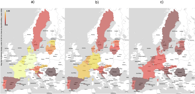
Description: These maps show each state’s number of differentiable crop classes when considering HCAT levels 6 (a), 5 (b), and 4 (c) (i.e., number on the diagonals of Supplementary Table 3, Supplementary Table 4, and Supplementary Table 5). A different way to obtain these numbers is by counting the maximum number of leaves (or most outer nodes) in the tree structure of Fig. 1 for each country. Level 6 includes all nodes; in case of level 5 and 4 the first respectively first and second outer rings are pruned off, and the resulting nodes represent the corresponding leaves. In some countries (e.g., Romania), most outer ring/level corresponds to level 4, which is why their counts don’t change when adding or removing hierarchy levels 5 and 6. In the case of Belgium, Germany, and Spain, the data was taken from the subregions for which, at the time of development, data was already provided. In this visualization, the range of the legends stays the same across all three maps, highlighting the increasing similarity of the set of crop types with decreasing HCAT levels. If the highest level of detail is chosen, the heterogeneity in sets of crop types is at its maximum, as shown in map (a). The more homogeneous crop taxonomies at level 4 (map (c)), enable larger spatial coverage in transnational analysis.

Full size image

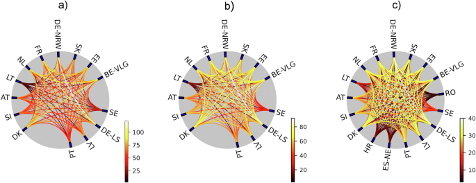
Description: The listed numbers of similar classes between two countries for HCAT levels 6 (a), 5 (b), and 4 (c) (corresponding to Supplementary Table 3, Supplementary Table 4, and Supplementary Table 5) are visualized in three-chord diagrams: Each bilateral connection is colored according to the similarity of crop taxonomy between the respective countries (EE Estland, SK Slovakia, DE-NRW North Rhine-Westfalia in Germany, FR France, NL Netherlands, LT Lithuania, AT Austria, SI Slovenia, DK Denmark, HR Croatia, ES-NA Navarra in Spain, PT Portugal, LV Latvia, DE-LS Lower Saxony in Germany, SE weden, RO Rumania, BE-VLG Flanders in Belgium). Yellow-to-white connections indicate high shares of common crop types in two countries’ taxonomies; red-to-black connections imply lower degrees of similarity.

Full size image

Case study

To showcase the potential of HCAT in facilitating research on crop-related diversity, we conducted a case study comparing crop diversity between exemplary regions at different HCAT levels (see Methods). For seven regions and the HCAT levels 4, 5, and 6, we calculated Shannon diversity ({{rm{H}}}_{{rm{i}}}) and the number of crop types ({{{n}}}_{{{c}},{{i}}}) for grid cells of 1 km × 1 km (Supplementary Fig. 1 and Supplementary Fig. 2). Having applied the same color scale across each metric, it can be observed that on average both the Shannon index ({H}_{i}) and the number of crop types ({n}_{c,i}) decrease with a lowering HCAT level. Further, we can see large differences for both metrics within (e.g., Austria and between regions (e.g., Navarra compared to Slovenia). The magnitude of these intra- and transregional differences appears to reduce, i.e., the regions increasingly assimilate and homogenize, with decreasing HCAT levels. These visual trends can also be quantitively observed for ({H}_{i}) and ({n}_{c,i}), in Supplementary Fig. 3 and Supplementary Fig. 4. With a few exceptions, we can see similar trends across the two considered metrics: Flanders stands out with the highest arithmetic mean value compared to Slovakia with the lowest values (Fig. 4, Supplementary Figs. 3 and 4). Austria shows the highest variability within the country, given in terms of the standard deviation and the extended interquartile range (whiskers range in boxplots). Figure 4 also quantitatively confirms the above-mentioned qualitative observation of a generally lowering heterogeneity between countries with decreasing HCAT levels. There’s also a distinct exception observable from the overall similar trends for the two metrics: Austria and Slovenia stand out with significantly lower mean values for ({H}_{i}) than for ({n}_{c,i}) compared to the other regions.

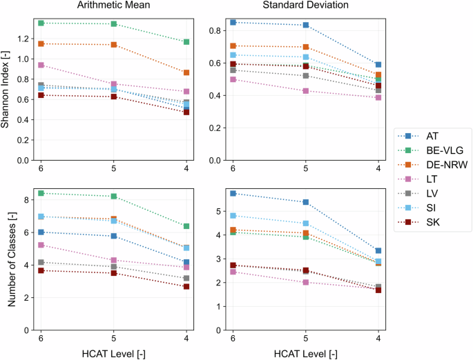
Description: Line graphs visualizing crop diversity per unit of area using arithmetic mean and standard deviation of the Shannon index H_i and of number of classes n_c,i per country and HCAT-level (4, 5, and 6) for seven considered regions/countries (AT Austria, DE-NRW North Rhine-Westfalia in Germany, LT Lithuania, LV Latvia, SI Slovenia, SK Slovakia, BE-VLG Flanders in Belgium).

Full size image

The number of crop types ({n}_{c,i}) represents an important factor for the ({H}_{i}) index. Yet beyond, also the size and number of fields per area (here discrete grid cells) influence the ({H}_{i}). Using Fig. 5 and Supplementary Fig. 5, we can observe that the regions differ partially significantly from each other with respect to the spatial characteristics of their agricultural landscapes, with some showing more than five times the average field sizes compared to other regions (e.g., Slovenia compared to Slovakia). The number of fields per grid cell generally shows an inverse trend compared to the median area of fields, i.e., regions with a relatively higher number of fields per grid cell show comparably smaller field sizes. It can further be observed that the number of crop types ({n}_{c,i}) correlates with the number of fields per area with a mean correlation coefficient of ({r}_{rm{mean}}=,0.70), and a certain heterogeneity within the considered scope or regions ranging from ({r}_{rm{LV}}=,0.61) to ({r}_{rm{SK}}=,0.76).

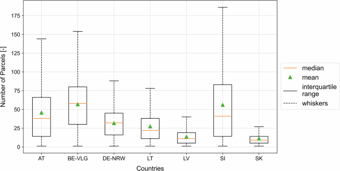
Description: Boxplots showing mean (green triangle), median (orange line), 25–75% interquartile range (IQR) (black lined box), and whiskers value range (dashed lines), defined as IQR ± 1.5 times IQR, of a number of parcels for the defined unit of area for seven considered regions/countries (AT Austria, BE-VLG Flanders in Belgium, DE-NRW North Rhine-Westfalia in Germany, LT Lithuania, LV Latvia, SI Slovenia, SK Slovakia).

Full size image

Despite the necessity of more quantitative information on farming activities and even though data on crop types are publicly available in the EU, there is today no structured taxonomy for administrative crop type notations across countries from multilingual language areas (see Introduction). With HCAT at hand, each EU country’s original, georeferenced parcel data can be enriched towards an extended version that additionally includes a direct translation of the crop type and the corresponding assignment to its corresponding HCAT class with name and identifier. Such enriched, harmonized data sets overcome the persisting language barriers (due to national-specific crop declarations) and can then be combined for transnational analysis.

Due to its hierarchical structure, HCAT allows for high flexibility during study design. The finest hierarchical level keeps the highest degree of detail. Decreasing the HCAT level entails a reduction of detail in crop denominations, and consequently introduces a loss of information. At the same time, the share of similar classes between countries increases, which enlarges the spatial potential for transnational analysis. To date, some countries/regions (Croatia, Navarra (Spain), and Romania) have only reported their taxonomy at a degree of detail corresponding to HCAT level 4, which enables transnational analysis including these countries/regions only at this coarser level of detail. Depending on their research objectives, scientists must carefully consider in advance to which spatial extent they want to use the data and which specific crop types they target, and accordingly identify the suitable HCAT level. Having outlined the significant potentials of HCAT for transnational, ecological studies in the EU, we, however, also want to discuss the currently given limitations and challenges of the taxonomy and the related usage of IACS data:

Despite IACS data often being utilized as reliable reference data for remote sensing applications^25,30,31, its limitations regarding correctness due to fraud or mistake need to be addressed and considered. Even though expert interviews with some control agencies in Germany have revealed empirical correctness levels above 95%, there is no official guarantee of EU-wide consistency in these terms. Consequently, analysis building upon the IACS data must be treated carefully, and methods applied that are robust to probably low but potentially existing declaration errors. Here the large size of the EU-wide EuroCrops data set offers an inherent countermeasure, as the relative importance of individual errors decreases with increasing data sets. Additionally, the subsidy does not rely on all crops cultivated over a year, so data collected within CAP usually only holds the primary or first crop grown on a particular parcel. Most of the time, this is enough information, but often, especially in warmer climates, it is known that there are several crop-growing cycles within one vegetation period. Any analysis that relies on the knowledge of conducted crop rotation is therefore limited to the presented type of data. Some member states like Austria and Portugal nevertheless have decided to release this information additionally, and even though we were not able to incorporate that into the vector data, we still attempted to provide translations to all specified crop types.

Regarding translations, it is also worth noting that even in the era of online dictionaries, most translation programs still struggle with national-specific agricultural terminology. This way, mistranslations soon became the central issue of the harmonization process and still hold the most significant potential of false classification of crops. Fortunately, several countries (Belgium, Croatia, Denmark, Estonia, France, Germany, Latvia, Portugal, and Slovenia) have decided to actively support us by providing corrections and feedback to our translation approach. Consequently, for these countries, the likeliness of mistranslations is at its lowest compared to other EU countries. The lowest error rates can also be expected for the most frequently and commonly cultivated crop types. To enable the possibility for individual quality assurance of HCAT-based experiments, we always provide the mapping of the HCAT classes next to the original, country-specific crop-type denominations.

Moreover, we also collected feedback from several collaborating institutions and potential users of HCAT regarding the taxonomy itself and provided them with discussion points for which we needed clarification. On purpose, stakeholders were chosen from different disciplines to help build the bigger picture of requirements. As expected, the results were laying on the entire spectrum of answers which resulted in the acknowledgment that there was not this one singular way satisfying both, e.g., the remote sensing community uniting with their focus on similar hyperspectral reflectance values of crops and the biologists with their clear-defined families and species of plants. Eventually, we decided to go for a compromise that both worlds might not consider perfect but are anyways willing to use and integrate into their domain-specific schemes. Independent from the applied compromises, if required, user can always identify the initial crop types through the provided raw crop denomination in their original and English language.

Across the above-mentioned aspects, we can see that HCAT fundamentally depends on the collaboration of the individual member states regarding the public provision of data and clarifications of national, domain-specific knowledge. So far, the majority of collaborating states are located in central and northern Europe. Contributions from southern and eastern EU countries would, therefore, be particularly beneficial for advancing the spatial representativeness of HCAT across the entire EU in future versions. Besides the quantity of data, we also encourage each country/region to further revise and enhance their ontologies, especially those countries that still report only at a coarse level of detail (e.g., Croatia at HCAT level 4). Yet, it’s also the public user and research community, which constantly contributes to improvements by providing feedback directly or via our community platform on GitHub³⁶. Among others, on this platform we provide latest updates on HCAT, users can share their suggestions and questions publicly via “Issues” or “Discussions”, or directly propose edited file versions via Git. Being maintained still for several more years, the EuroCrops project warmly welcomes further reviews and contributions specifically for version 3, currently under development and generally for improved, future HCAT versions. By letting HCAT evolve over the past years and being open to discussions and feedback, it was possible to develop a scheme that shows the possibility of building a meaningful transnational taxonomy that holds more classes than all previous attempts. The hierarchical structure, open-data policy, and substantial spatial and linguistic coverage represent key characteristics of a scheme that is unprecedented in the field of crop taxonomies.

Relating to applications of HCAT for agricultural and ecological studies, literature shows that precise knowledge of the presence, variety, and spatiotemporal organization of cultivated crops in a landscape can be a significant information source for elucidating ecological conditions and fluctuations on national and transnational levels. To outline technical considerations when working with HCAT and to demonstrate the usability of HCAT for crop-related diversity assessments, we conducted a case study comparing crop diversity at a landscape scale across seven EU regions. Having harmonized the national-specific datasets with HCAT, we first performed a comparison of crop diversity based on the Shannon index ({H}_{i}) and the number of crop types per spatial subunit ({n}_{c,i}) (here: 1 km × 1 km grid cell). We could thereby observe intraregional and interregional patterns in crop diversity, which both decreased in heterogeneity with lower HCAT levels. On an intraregional scale, this is an expected behavior as the overall number of crop types in each region’s taxonomy reduces with decreasing HCAT levels. On an interregional scale, this also holds true as the taxonomies increasingly align with each other with decreasing levels of detail in the crop-type denominations (see Fig. 3).

Taking the complete selection of regions without prior assessments allows, in any case, for studying qualitative trends between and within regions at varying HCAT levels. However, for a quantitative comparison of crop diversity across several regions, the scope of regions must be carefully selected with respect to the total number of crop types in their national declarations. As Supplementary Table 2 outlines, the number of crop types reported ranges from 15 in Croatia to 326 in the Netherlands. A comparison of the crop diversity as reported by the countries inevitably shows much lower crop diversity values for Croatia than for the Netherlands. Such differences can also be observed in the case study when comparing Lithuania (LI) with 24 classes compared to Flanders in Belgium (VLG) with 274 (Supplementary Figs. 1 and 2). There are two possible interpretations for these differences: (1) the diversity of cultivated crops is in reality higher for countries or regions such as Flanders in Belgium, or that (2) countries with a low number of crop types in their declaration taxonomies do not specify crop cultivations as detailed as others. Consequently, there would be a bias in the data when countries provide crop declarations only on a broader level, even though farmers might, in practice, cultivate more diverse sub-types.

Our case study provides evidence for both scenarios by documenting a variation in the similarity between regions when using crop types at higher HCAT levels (e.g., Lithuania compared to Austria (Fig. 4)) and also regions where the differences in crop diversity are apparent in all HCAT levels (e.g., Flanders and Slovakia). In the first case, differences in measures of crop diversity result from differences in the level of detail at which countries report the data and do not reflect real-world differences. In the latter case, differences in measures of crop diversity reflect differences in what farmers plant in the real world. Thus, when using these measures of crop diversity, e.g., as predictors in studies of biodiversity, we would expect meaningful relationships only in the latter case. Therefore, the similarity of crop declarations is an essential factor in the study design and evaluation process of studies relating, for instance, to biodiversity farming practices in studies that include areas of more than a single EU national state. Despite the Shannon index being defined both by the number of crop types per area and a factor describing spatial characteristics, interestingly, many regions (6 out of 8) strongly followed the patterns of the pure ({n}_{c,i})-based approach. Two countries (Austria and Slovenia) ({H}_{i}) indices were also dominated by spatial factors instead, showing deviating patterns compared to the other regions and the ({n}_{c,i}) -based approach. These observations outline that knowledge of the presence of cultivated crop types is key in the context of crop diversity assessments, but they also confirm literature’s reports on the importance of deriving landscape crop diversity together with its spatial characteristics^6,16,17,18. This further highlights the significance of joining HCAT with geodata, as it is established within the harmonized geodata set EuroCrops, which combines both spatial and harmonized crop data. HCAT served in this study as an accessible and user-friendly tool for analyzing crop management patterns in agricultural landscapes across various regions within the EU. These regions apparently exhibit distinct variations, which originate in practice from their characteristic socio-economic and geographic circumstances and, at an administrative level, from a country’s specific crop declaration system.

The presented case study concentrated solely on evaluating crop diversity, and on highlighting technical considerations when working with HCAT. We must emphasize, however, that with our chosen study design, there can not be drawn direct conclusions on biodiversity drivers without additional adjustments. This is mainly because we included all available crop types ranging from temporary, productive crops to permanent, non-cultivated vegetation types. Such an approach leads to an untraceable mix of crops regarding these two influential extra categories of cultivation intensity and retention period. Indeed, high values for our chosen crop diversity indices in one intensely cultivated area would indicate potentially more beneficial conditions for natural species compared to another area given the same level of cultivation intensity. Yet, areas with large, extensively cultivated, or even non-cultivated fields would show low crop diversity values but actually provide more beneficial conditions for biodiversity compared to highly crop-diverse but intensely managed fields. Consequently, for robust results, the selection of HCAT classes needs to be adjusted beforehand to a study’s application-specific objective by, e.g., additionally considering biodiversity-related factors, including habitat structure, cultivation intensity, or food resources.

We gave an idea of HCAT’s usage in the context of biodiversity research, yet HCAT’s low level of customization also offers potential for application in various other domains. HCAT can serve as a flexible starting point towards thematic taxonomies using domain-specific extensions. These extensions may include thematic extra attributes, e.g., as in the FAO’s ICC taxonomy³⁴, which would provide additional parameters for more customized application-oriented filtering or restructuring of the underlying data set. Taking the example of the three dimensions of sustainability, these extensions could range from economic masks that facilitate the evaluation of EU-wide food safety via social analyses on farm structures to tailored environmental studies on biodiversity considering the above-mentioned aspects. With the release of HCATv2, the EuroCrops project now increasingly intensifies communication and promotes the application of its results into various domains. Developing thematic taxonomies alone goes, however, beyond the current project team’s capacities and expertise; EuroCrops, therefore, encourages each discipline to interact with the project team and the HCAT community for discussions and collective developments on domain-specific extension forms (e.g., via the HCAT-GitHub repository³⁶). The exemplary assessment of crop diversity represents a showcase of HCAT’s applicability, we, however, want to highlight that the main result of our work is the taxonomy itself. Despite the mentioned limitations, this second version of HCAT offers significant potential for transnational analysis of spatiotemporal crop heterogeneity, diversity, and the structure of agricultural land, and by this, a meaningful source of information for transnational research on agricultural practices and related sustainability impacts.

Data collection

Within the scope of the EuroCrops project, data from the EU’s Integrated Administration and Control System (IACS) was collected to compile a transnational dataset for crop type classification³⁵. Depending on a country’s policies, it is possible to obtain geodata and related crop-type declarations via public websites or Web Feature Service (WFS); however, it was often necessary to contact the agricultural authorities directly. One integral property of the EuroCrops initiative is open and FAIR³⁷ access to all collections. We, therefore, ensured and communicated that all data given to us will be distributed under the Creative Commons Attribution International license CC BY-SA 4.0. After over one year of extensive outreach and communication, the resulting pool of gathered data exceeded our expectations: 13 countries and four subregions from three more countries contributed to the HCATv2 development by providing their geodata-based crop declarations including their national/regional crop taxonomies (compare Supplementary Table 2 and Fig. 2). The remaining EU members states were still in process or denied to publicly share the data. In theory, having the possibility to use a large-scale unified dataset could build the foundation of an endless number of applications and use cases, especially in machine learning and data-driven modeling. However, publicly available crop data naturally comes in the national language of the respective country and uses country-dependent agricultural terms, leaving even common translation programs clueless. Supplementary Table 6 gives an insight into the original data and highlights the importance and need for a common crop taxonomy when designing transnational studies. The HCAT-enriched version of this original data is displayed in Supplementary Table 7, showing the additional HCAT-specific attributes comprising a translation, unique name, and code.

The development of HCATv2 required a volume of data that (a) aimed towards a large and geographically diverse as possible coverage of the studied area, i.e., the European Union, and (b) is lightweight enough for reasonably fast processing. We therefore decided to use only selected periods of the comprehensive multi-year and multinational EuroCrops database: from the period 2018–2021 we selected for each country the one, most recent year of IACS data being available at the time of data collection in mid-2021. Apart from the original situation of some countries having published their data for only a single, or few, non-consecutive years, there’s also the aspect of some countries having released national datasets in retrospect with distinct delays (e.g., France). This is why the chosen base years for HCATv2 (a) can differ between countries/regions, and (b) may also deviate from the one that would be chosen based on the nowadays available database for the considered period. From this data collection, we subsequently extracted all available crop-type classes. The latter represents the set of data on which HCATv2 is based. Supplementary Table 2 displays the considered year for each country and gives an overview of the total number of crop parcels and occurring classes. The extensive list of each country’s original crop types with their corresponding HCAT equivalents is publicly available on the EuroCrops’ project GitHub repository³⁶. It is constantly updated with additional years and newly participating countries, serving as the basis for further extensions and improvements in future HCAT versions.

Transnational crop class harmonization

During the development of the EuroCrop project’s first demo dataset²⁴, we were inspired by the already existing EAGLE classification scheme³² for the structuring of crop types. This scheme provides a broad hierarchical approach for the categorization of land use and land cover types ranging from natural biotic and abiotic to various anthropogenic land cover components. At the time of development, we found, however, a significant shortcoming in the EAGLE taxonomy regarding the scope and level of detail of crop types. We, therefore, already genuinely extended the EAGLE scheme by adding frequently occurring crop classes, leading to a first version of the Hierarchical Crop and Agriculture Taxonomy (HCATv1) as first presented in 2021²⁴.

Underestimating the demand for the proposed dataset and the variety of use cases, feedback taught us that the initially proposed scope of crop classes in HCATv1 needed more coverage and detail and made us rethink the entire process again. For HCATv2, we aimed to keep as much information as necessary while reducing the overhead as much as possible. In our case, this resulted in an iterative process of mapping almost all translated crop classes that we could obtain from collaborating countries and regions to our best knowledge to a dynamically growing extension of HCATv1. This time, we put a stronger focus on the hierarchical structure of the cultivated crop classes regarding land use, land cover, and biological families. Eventually, the number of classes increased from previously less than 100 to over 350. Despite this further extension of classes, there is still some inherent abstraction in the scope of crop types, as we summarized some rarely occurring, very similar, and/or single country-specific classes into related, overarching crop types. All original crop notations can, however, still be retraced using the provided original and translated name.

In the updated hierarchy, the sixth level entails the highest degree of detail. With decreasing numbers, the denominations for crop types become coarser (e.g., winter barley (level 6) ⊂ barley (level 5) ⊂ cereal (level 4) ⊂ arable crops (level 3)), with the third level representing the coarsest level that still differentiates between crop classes. HCAT levels 2 and 1 are given by the position of crop types within the EAGLE taxonomy version 1³². In this EAGLE version, crop types are classified into the category “Crop Type” (level 2), which itself is part of the category “Land Characteristics” (level 1), both being numbered by the digit 3 in their respective hierarchy layer. Consequently, we defined each of the HCAT codes to begin with the prefix “33” (see column EC_hcat_c of Supplementary Table 7), indicating this placement into the higher-level land use and land cover context.

Case study: cultivated crop diversity in Europe

To showcase the practical application of HCAT in research on crop-related diversity, we designed a case study focusing on assessing crop diversity across seven EU regions at a landscape scale. The specific subgoals of this study were to identify distinctive patterns (1) in relation to different HCAT levels and (2) between each other. Moreover, the study serves to highlight key factors that should be considered when conducting crop diversity assessments using HCAT. The initial selection of countries/regions was influenced by the public availability of national data sets and the intention to include representatives from various areas of the EU, including countries from the Atlantic region with the German federal state of North Rhine-Westphalia and Flanders in Belgium, the Continental region with Austria and North Rhine-Westphalia, the Boreal region with Lithuania and Latvia, Alpine areas with Austria and Slovenia, and Pannonian region with Slovakia. Exhibiting limited crop reporting at only HCAT level 4, we could not incorporate the regions/countries Navarra, Croatia, and Romania, which otherwise would geographically depict suitable representatives for the Mediterranean and Steppic regions. The same holds for Portugal, which shared its national taxonomy with us but has not provided the necessary geodata so far. The mentioned regional classes originated from the Biogeographic Regions classification scheme of the European Environment Agency. Areas within these regions exhibit similarities encompassing factors such as climatic conditions, geological attributes, and vegetation patterns³⁸.

In the first step, we harmonized each region-specific EuroCrops-sub dataset of original crop declarations by extending these with the HCAT crop declaration. To compare across several HCAT levels, we created three duplicates per region—each with a different HCAT level ranging from 4 to 6. After this step, a country’s overarching, application-specific filtering of crop types would be seamlessly possible. For our application independent calculation examples, we took the entire scope of available crop types, including temporary crops, but also permanent cultivated and non-cultivated types. Next, in order to have a common spatial resolution for transregional/-national statistical comparisons, we split each region-specific dataset into grids of 1 km × 1 km cells. This process was done by first constructing vector-based grids that span the entire area of each respective region; afterward, we intersected each grid cell with the vector-based parcel data. After these pre-processing steps, we iterated for each of the 24 combinations of scales (8 regions times 3 HCAT levels) over all the grid cells and derived statistical metrics, including the number of parcels in a grid cell, the contained area of each parcel, and the list of cultivated crop types for each cell. We chose the number of crop types in a grid cell ({n}_{c,i}) as one measure for exploring each region’s crop diversity across the three different HCAT levels. ({n}_{c,i}) represents a metric that allows for quick qualitative estimation of crop diversity without additional calculations. It, however, neglects both number and area-wise distributions of samples inside each cell’s population of crop parcels, which are likewise influential factors to crop diversity at landscape scale (see Introduction). Relying only on ({n}_{c,i}) might, therefore, lead to insufficient results during quantitative diversity assessments, which is why we decided to also calculate the Shannon index(,{H}_{i}) for each grid cell (i). ({H}_{i}) represents a common diversity index, which describes, in our case, the diversity of crop types, considering both the number of crop types and their abundance, expressed here through the relative area in the grid cell³⁹. It is defined as

with

where ({p}_{k,i}) denotes the ratio of each crop type (k)’s area ({{n}}_{C,i,k}) in grid cell (i) and the total area of samples ({N}_{{C}_{i}}) in grid cell (i). To answer the described study objectives, we calculated descriptive statistics for each region’s ({n}_{c,i}), ({H}_{i}), as well as the number of parcels and the median field area per grid cell as potential indicators for spatial variability. We applied a common color scale to each metric’s set of maps to reveal the quantitative differences between considered countries.