AI-guided framework for the design of materials and devices for magnetic-tunnel-junction-based true random number generators

Introduction
Designing application-driven devices is oftentimes a time rigorous and resource-constrained process that requires utilizing computationally intensive simulations, device fabrication, and testing of the physical components in the application-specific environment. At the same time, customizing device characteristics to a particular application can allow for performance improvements. Automated codesign strategies are becoming increasingly popular with advancements in the artificial intelligence (AI) field that provide useful machine learning algorithms and frameworks1,2,3,4. Such codesign provides new opportunities to automatically customize devices for application-specific needs to maximize performance—whether that involves a particular capability, energy usage, latency, throughput, or even combinations of metrics. The operation of emerging devices, such as magnetic tunnel junctions (MTJs)5,6,7,8, can be simulated using physics-based models that capture key behaviors based on materials and device properties. By pairing these models with AI-guided codesign, we are able to effectively optimize the device parameters for application requirements and constraints9,10,11.
AI-guided methods are increasingly being adopted in electronic design automation (EDA) flows. Recently, reinforcement techniques have been used in EDA for multiple tasks including chip floor planning12, architecture search2, gate sizing of VLSI13, circuit optimization14 and analog circuit design15. Evolutionary algorithm (EA) approaches, on the other hand, have been used for decades to design analog circuits16 and can be creative in the design of unique solutions to a variety of problems17. Both reinforcement learning (RL) and EA approaches are promising for optimization tasks, each offering unique pros and cons. In addition, recent work leverages generative AI-based circuit characterization18 and optimization techniques19,20. In related work, physics-informed neural networks21, originally designed for solving partial differential equations with informed loss functions, have been used to perform device design and optimization22,23,24. Codesign across devices, circuits, architectures, and applications for a full-stack solution is a challenge and an ongoing area of research.
In previous work, we have shown initial results in leveraging RL for MTJ device codesign10 and EA for probabilistic circuit optimization using different MTJ devices and tunnel diode device9. This work presents an intelligent, automated codesign framework for emerging devices. In particular, we create a framework that is based on RL and EAs, which allows for multi-objective optimization of parameters of emerging devices for real-world applications. We showcase this framework by providing a comparison of RL and EA approaches for device design and parameter optimization and a demonstration of device parameters for energy-efficient random number generation for gamma distributions for both spin–orbit torque (SOT) and spin transfer torque (STT) MTJ devices. Though this framework is applied in the context of true random number generation using SOT and STT MTJ devices, it can be easily extended to other applications and other device types.
Ultimately, our methods produce the best candidate devices and materials properties for optimizing both performance in function and energy efficiency. Generally, we see that performance is improved but energy efficiency is slightly increased, compared to the default parameters used to represent standard CoFeB MTJs. The results also show that for the SOT MTJs, a larger range of material parameters can provide good performance, and material parameters for stronger perpendicular magnetic anisotropy (PMA) are favored. In contrast, for STT MTJs there is a narrower range of parameters to achieve the performance, and weaker PMA is favored.
Methods
Application: true random number generation for non-uniform distributions
To guide the development and discussion of our codesign framework, we focus on a single application—true random number generation (TRNG), Fig. 1c. Despite this focus, we stress that our presented framework is general purpose for the AI-guided design and configuration of devices to meet application needs. Here, our devices are both SOT and STT MTJ devices. Our target function for these devices is to produce TRNG samples from a distribution of interest.

Overview of the device model, AI-guided discovery and optimization strategy, and RNG algorithm workflow. Given a target distribution, the optimization approach (b) uses a device (spin–orbit torque or spin transfer torque) model (a) to simulate a true random bit according to the RNG algorithm (c). The optimization algorithm designs unique device configurations (d) that must pass device checks to be viable. The viable devices are used to produce the target distribution for a given application (e).
Random number generation is a key component of many computational tasks, including scientific simulations, machine learning, and cryptography. In today’s computing systems, random numbers are typically generated using pseudo-random number generators (PRNGs), which have several key limitations, including the quality of the random numbers generated (e.g., adherence to expected distributions or predictability) and periodicity of outcomes. Furthermore, many PRNGs are restricted to generating samples from a uniform distribution; if an application requires pseudo-random numbers from a different distribution, then additional computation is required to convert the sampled number to the appropriate distribution.
Recent studies into microelectronics and probabilistic computing have noted the need and potential for fast and efficient TRNG and noise sources25,26,27,28. A step beyond random bits, as indicated in ref. 25, is to produce samples from specified distributions of interest, eliminating the need for expensive rejection sampling. This motivates our decision to focus solely on drawing from a specified distribution of interest. While we elect to focus in on a single distribution, our prescribed framework can apply to any distribution that admits a tractable distribution. Additionally, since our devices are acting as biased coins, popular benchmarks to test the RNG quality, such as NIST, aren’t applicable.
We choose to focus on a particular distribution in the gamma family. The gamma distribution is a natural generalization of the exponential distribution. It is applied in a variety of applications, including mathematical ecology (population and epidemic modeling), industrial systems engineering (queuing theory and related service time modeling), and finance (default modeling). While the exponential distribution represents the waiting time of a single event arriving at a rate λ, the gamma distribution can be thought of as the waiting time for n arrivals of events that individually arrive at a rate λ. The two parameters of the gamma distribution are the shape n and the rate λ. The exponential distribution arises as the special case when n = 1. Both parameters can take on any positive value.
For this effort, we selected n = 50.00 and λ = 311.44. This target distribution, shown in Fig. 2a, provides features not present in a simple exponential. Namely, it provides an asymmetric shape tightly concentrated around a single value. These features and the entire codesign framework dramatically differentiate this work from existing literature applying vanilla RL to a vanilla exponential distribution9,10,29. For explicit details on how we selected these values and an application to particle tracking, please see Supplementary Note 1.
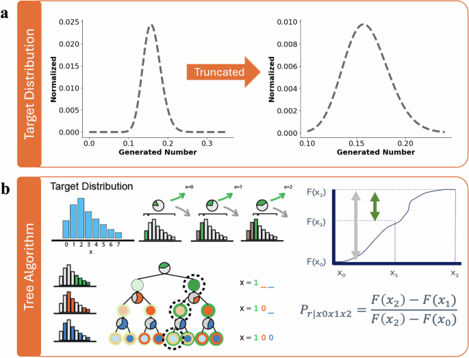
Truncated target distribution (a) is used in the tree algorithm (b) to optimize the MTJ devices to match the desired distribution.
In the context of our codesign workflow (Fig. 1), we will need an algorithm that transforms output from stochastic devices to samples from distributions of interest. This is the RNG algorithm and it is the object (or function) of interest, informing the behavior of our devices and prescribing a need to precisely control their stochastic profile. In general, this choice of algorithm is a step in our framework for device design and can be arbitrary.
The RNG function we chose provides a binary-coded random number according to the desired probability density function (PDF) by utilizing output from tuned coinflips. Prescriptively, we begin with a PDF supported on some finite interval [a, b]. If the PDF is not finitely supported, we truncate it in a negligible way and renormalize. Our selected gamma distribution is not finitely supported. Hence, we will need to truncate the infinite support. We truncate our PDF to the interval [0.10, 0.24]. This interval contains ~99.79% of the mass of the distribution and is illustrated in Fig. 2a. Our selection for the bounds of the truncation was arbitrary, but our methodology would still be valid for any finite range. Note, with our RNG algorithm of choice (discussed in the following paragraph) there is no possibility of returning values outside the truncated range, even with noise imparted by the device.
Once we have an appropriate PDF, we construct a sampling decision tree by discretizing the PDF. For a k-bit number, we divide the chosen interval [a, b] into 2k equally-spaced bins. Note, bins need not be equally spaced, but for ease of discussion, we assert that each bin has the same extent. We create a binary flip tree encoding the outcomes of each of these bins from a sequence of coin tosses. The first coin toss will have a probability of tails equal to the integral of the PDF from a to (a + b)/2. This partitions the probability of the first 2k−1 bins and the second 2k−1 bins. The second layer of the tree comprised two weighted coins. The first coin has a probability of tails equal to the integral of the PDF from a to (3a + b)/4. The second coin has a probability of heads equal to the integral of the PDF from (a + 3b)/4 to b. This process is continued until the final layer, where the integration is performed over the width of a single bin. In total, there will be 2k − 1 weighted coins. In practice, the coin in the topmost layer is flipped; depending on the outcome of the first toss, a single coin in the second layer is selected to toss. This process continues.
In contrast to precomputing all 2k − 1 coin weight values in the full probability tree—a process that grows exponentially with the desired bit precision—we instead modify the scheme and utilize an online process. We traverse through only those branches of the probability tree that are relevant for each sample by exploiting the cumulative distribution function (CDF). This scheme is suitable for any distribution for which the CDF can be defined. For our gamma distribution, we merely integrate our truncated PDF for x ∈ [0.10, 0.24] to obtain our CDF.
Let F denote the CDF of a desired finite distribution on some interval [a, b]; that is, (F(x)={mathbb{P}}[Y , < , x]). In an online fashion, the first coin weight is determined by evaluating
This coin is then flipped. If the outcome is 1, for example, then the next coin weight is determined by evaluating
Since this process is online, the weight of the next coin flipped depends on the outcome of the previous coin. Based on that outcome, the interval of integration (the evaluation points in the denominator) and the midpoint of the integral (the second evaluation of F in the numerator) change dynamically too.
Compactly, if we let b represent the binary representation of the output random number, we can define the probability that the kth bit of b will equal 1 as
where x0 and x2 represent the endpoints of the current interval and x1 represents the midpoint. By dynamically setting x0, x1, and x2 as successive locations according to the outcome of the previous coinflip, we can progressively sample a binary-coded digit from an arbitrary CDF.
Using this approach, we use a simple recursive algorithm that dynamically sets x1 and x2 depending on the outcome of the previous coinflip bk. If bk = 1, then we move the lower bound to the current probability threshold, x0 ← x1. Likewise, if bk = 0, we reset the upper bound (x2 ← x1). Next, we compute the next as the halfway point between the upper and lower bounds (x1 ← (x2 − x0)/2). This process is illustrated in Fig. 2b.
Device models: magnetic tunnel junctions
The second component of the codesign framework includes the device models, Fig. 1a. We utilize physics-based models of these devices to accurately capture the device behaviors based on the device and material properties. This allows us to effectively optimize the devices to target desired distributions while considering additional constraints such as energy efficiency. This component can be updated to explore numerous devices using various modeling techniques, whether it be physics-based models, machine-learning models, or incorporating physical device readings. This flexibility allows the framework to optimize for multiple devices regardless of the modeling approach.
We use a numerical model of MTJs based on a macrospin approximation of the Landau–Lifshitz–Gilbert (LLG) equation30,31, modeling a standard MTJ stack with PMA comprised CoFeB (free layer)/MgO/CoFeB (fixed layer). This MTJ stack can be operated in different modes for TRNG; an SOT-MTJ device is shown in Fig. 3a. In the SOT operation, an applied JSOT current in a heavy metal layer beneath the stack rotates the magnetization of the free layer (FL) to be in-plane via the spin Hall effect, then removed for relaxation, as the free layer settles to its PMA lowest energy state to either the 1 or 0 states. This process can be biased using an applied JSTT current through the stack. The model is developed in Python and FORTRAN and accounts for device-to-device variability expected for state-of-the-art magnetic random-access memory (MRAM)29,32. An example computed SOT S-curve is shown in Fig. 3b relating the biasing current JSTT to the bit probability, and two example random bitstreams are shown in Fig. 3c. These bitstreams were produced with extrinsic parameters, applying charge current density of amplitude JSOT = −4 × 10¹¹ A/m2 without field assist, pulse duration of 10 ns, followed by relaxation of 15 ns. The chosen material parameters for ferromagnetic CoFeB are damping constant α = 0.03, anisotropy constant Ki = 1 × 10⁻³ J/m2, saturation magnetization Ms = 1 × 10⁶ A/m, and spin Hall angle η = 0.3. Detailed device parameters are shown in Table 1. We leverage this model29 for optimization experiments at room temperature (T = 300 K) in the next section to codesign the device as a TRNG for a gamma probability distribution function.
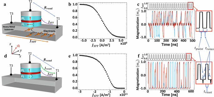
Schematic illustrations of the modeled spin–orbit torque magnetic tunnel junction (SOT-MTJ) (a–c) and spin transfer torque magnetic tunnel junction (STT-MTJ) (d–f) with perpendicular magnetic anisotropy. a The SOT charge current (JSOT) is applied through terminal T3 to T1 to rotate the free layer (FL) in-plane, and the change of magnetoresistance is read through an MTJ via terminals T2 and T1 after JSOT is removed. An additional STT charge current JSTT between T1 and T2 provides biasing of the coin. d The current (JSTT) induces a stochastic switching of the free layer, which is reset with Jreset after each read operation. b, e Example device S-curve showing how STT current amplitude (JSTT) between T1 and T2 biases the bit probability for both device types. c, f Two example random bitstreams generated using the simulation model29, with accompanying pulsed SOT or STT currents in units of mA.
Unlike the SOT-MTJ device, an STT-MTJ device does not require a SOT current to rotate the FL in-plane. Instead, the supplied STT current provides the entire mechanism for stochastic switching. Resetting the FL to be in the—z direction between each sample, an STT current through the stack has a probability to switch the FL depending on the STT magnitude. The STT operation is shown in Fig. 3d, with corresponding example S-curve and bitstreams in Fig. 3e, f. The STT device parameters to generate these bitstreams were the same as those listed for the SOT device, while the pulse, relax, and reset times for the STT are 1 ns, 10 ns, and 10 ns, respectively, and shown in the insets in Fig. 3c, f.
AI-guided codesign framework: reinforcement learning
The last component of the codesign framework includes the AI-guided codesign strategies, Fig. 1b. This work explores and compares both RL and EA to help determine the optimal parameter values for the materials and devices in order to display a desired distribution while accounting for additional constraints, i.e., energy efficiency. The codesign framework is flexible and extendable allowing the investigation of additional constraints to fit the requirements of the given application if needed.
RL is a class of machine learning techniques that trains an agent to learn optimal decision making for a given environment (the world the agent inhabits) in order to maximize its rewards33. The main control loop begins with the agent taking an action based on the observations available to it for a given state of the environment. The observations provide key information the agent may use to gauge its current situation to determine potential actions to take. The agent is then provided a reward that either penalizes or affirms said action and the environment is updated by transitioning to the next state triggered by the agent’s action as shown in Supplementary Fig. 1.
This state–action–reward dynamic is a crucial component of various RL algorithms. A popular branch of these algorithms is policy-based approaches which is what we are using in this work. This approach focuses on optimizing the policy which is responsible for providing the agent with optimal actions to take. We used a well-established RL algorithm called proximal policy optimization (PPO) by OpenAI for our RL algorithm34. PPO limits the policy change at each epoch to avoid large policy updates which helps to converge to an optimal solution by mitigating large, destructive policy changes.
For each of the device models solving for the RNG application, a similar RL setup was constructed to train an agent to optimize the materials and parameters of the two device models to best exhibit the desired distribution. To accomplish this, two metrics were leveraged to define optimal configurations: Kullback–Leibler (KL) divergence and energy. KL divergence helps determine how close one distribution is to another, and energy calculations relate to how efficient the device is. Therefore, to obtain the best configurations, the agent is trying to minimize both metrics.
To facilitate the RL optimization, we leveraged OpenAI’s RL framework, Stable-Baselines335. This framework allowed us to build a custom environment that integrates the device models to allow agents to explore the parameter search space to optimize against KL divergence and energy consumption. The framework also provides built-in RL algorithms which simplify the training process by easily allowing the switching of training algorithms, including the PPO algorithm we utilized. For both devices, the agent was trained for 6000 timesteps and then tested on 150 episodes with each episode consisting of 60 timesteps. For more information, refer to Supplementary Methods.
AI-guided codesign framework: evolutionary algorithms
Evolutionary optimization is an optimization approach inspired by principles in natural evolution. In evolutionary optimization, potential solutions are represented as genomes, and a population of genomes is maintained throughout the optimization. Each genome is converted into a phenome and evaluated through a fitness function, which corresponds to the objective function that is either minimized or maximized. Selection procedures are used to select parents from the population of individuals based on their fitness values. Then, reproduction operations such as random mutation are performed with the parents to produce children genomes, which then replace the parents. To allow for multi-objective optimization, we use the non-dominated sorting genetic algorithm II (NSGA-II)36. In NSGA-II, individuals are selected to fall along the Pareto front, with a crowding distance metric that is used to promote diversity among the selected individuals.
Here, the individual genomes in our population are real-valued arrays, where each gene in the genome represents the parameters of the device type. We use Gaussian mutations to mutate the real values in the array. In evaluating the device performance, we use two objectives: KL divergence and energy usage. The goal is to minimize both of those values—similar to the RL approach. If the configuration is invalid, then the KL divergence and energy usage values are set to a large value (1,000,000) to strongly discourage invalid configurations.
We utilized the Library for Evolutionary Algorithms in Python (LEAP)37 to facilitate our EA optimization. LEAP is a general-purpose framework for evolutionary algorithms that employs a pipelining feature for search and optimization algorithms with useful distribution and visualization features. They provide multi-objective optimization algorithms, including NSGA-II36 utilized in this work. The framework allows for easy modification of population, training generations, mutation, and crossover parameters—key aspects of evolutionary algorithms—which allowed us to test various training setups. For both devices, 25 runs were performed with a population size of 50 for 50 generations of evolution.
Note, all figures, graphs, and diagrams were created by the authors of this paper. The Matplotlib library in Python was used for graph creation, PowerPoint for flow diagrams, and Rhinoceros 3D for device visualizations.
Results
Reinforcement learning results
Figure 4 shows an overview of the results for our RL approach to device design. Figure 4a, b show the PDF comparisons for the SOT and STT devices, respectively. Each figure shows the distributions produced by the average of the top 5 devices generated through RL, the distribution produced by the best device configuration, and the result of the PRNG all compared against the target distribution. Note that the PRNG was sampled the same amount as the MTJ devices (100,000) to allow for comparisons. As can be seen in these figures, the optimized device results match well to the target distribution and are mostly consistent with what is seen for the PRNG. We can see in Fig. 4b that there is significantly more variation for the STT device than the SOT device, particularly with drift from the distribution of the generated numbers between 0.20 and 0.22. This is expected behavior, as the STT device stochasticity should be harder to tune due to having one control knob while the SOT device has two control knobs. While the SOT device needs its free layer to be brought in-plane and then allowed to relax, the current to flip the STT device needs to be fairly precise to achieve proper biasing. However, the tradeoff is added complexity and terminals to the SOT-MTJ compared to the STT version that can use a 1 transistor, 1 resistor STT-MRAM structure.
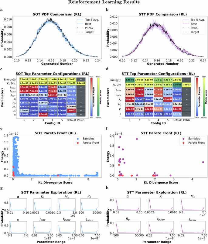
a, b PDF comparison of top 5 device configurations, best configuration, pseudo-random number generator (PRNG), and target distribution for both SOT and STT devices. c, d Parameter configurations of top 5 devices with energy and Kullback-Leibler (KL) divergence metrics compared against the default configurations and a PRNG for both SOT and STT devices. e, f Pareto fronts comparing energy and KL divergence metrics of various SOT and STT device configurations. g, h Probability distributions of the parameter ranges that were explored for both SOT and STT devices.
Figure 4c, d show the five best configurations discovered for the SOT and STT devices, respectively, along with their respective KL divergence and energy metrics. The top 5 devices are considered to allow comparison of configuration variability through the optimization strategies among the top performers. In order to provide a baseline, these optimized configurations are compared against a PRNG and “default” values for each device parameter, established through literature and prior works38,39,40,41,42. It is worth noting that the individual color ranges for the energy and KL divergence metrics were determined by looking at all device configurations (SOT and STT), for both automated codesign strategies (RL and EA), including the default configurations and the PRNG. The optimized configurations for both devices were able to outperform the default configurations in terms of KL divergence. However, the energy metric wasn’t improved upon from the default configuration, and this can be attributed to less weight being applied to the energy metric in the fitness score—increasing the weight can incentivize better energy efficiency. It is clear that there is not one set of parameters that leads to the best performance for a given device set, though there are trends for certain parameters. In particular, the Gilbert damping constant (α) is consistent across both the STT and SOT devices.
For the SOT device, the trelax and tpulse parameters tend to stay toward the high end of the allowed range, but the same is not true for the STT device, where there is more variation in the parameter values used in the top 5 devices. This indicates that it is worthwhile to customize the parameters for each individual device type. For the remaining parameters, values across the ranges are used for each of the top 5 device configurations for the STT device, but values toward the lower bound are preferred for the SOT device which may suggest the agent falling in a local optima. Looking at the energy and KL divergence metrics, we can see that the SOT device produced more energy-efficient configurations that more closely matched the target distribution compared to the STT device.
Figure 4e, f depict the Pareto fronts comparing energy consumption and KL divergence of the valid configurations for both SOT and STT devices, respectively. As seen by the figures, there are significantly more samples for the SOT device compared to the STT device. This suggests that there is a smaller subset of valid configurations for the STT device as opposed to the SOT device, as expected.
This disparity allowed for a larger exploration of the energy and KL divergence space for the SOT device, while the STT device has clusters of samples, suggesting that there may be fewer configurations that deviate too far from the desired distribution as seen by fewer occurrences of larger KL divergence scores. Nevertheless, both devices share a similar trend: closely matching the target distribution (lower KL divergence score) typically results in increased energy consumption. This tradeoff is a crucial element to be aware of when designing such devices since it offers a gradient of possibilities to best match the application requirements.
Figure 4g, h showcase the probability distributions of the parameter ranges that were explored through RL for both SOT and STT devices, respectively. From the graphs, we can clearly see that the majority of the parameter exploration took place at the bounds of the parameter ranges for both devices. This matches with the top parameters discovered (Fig. 4c, d), where the parameter values tend to be toward the bounds of their respective ranges. This suggests that the agent may have fallen into a local optimum; however, the Pareto fronts suggest that the agent was still able to discover a wide breadth of the performance metrics’ (energy and KL divergence) space.
Evolutionary algorithms results
Figure 5 provides an overview of the EA results for device design. Figure 5a, b display the PDF comparisons of the SOT and STT devices, respectively. Once again, we see that the device parameters discovered by the EA closely mimic the desired distribution and the distribution generated by the PRNG. Similarly to the RL results, we also see that the STT device has more variation from the distribution than the SOT device, but this time for generated numbers between 0.16 and 0.18, which indicates that different parameter sets may result in more variation at different points in the distribution.
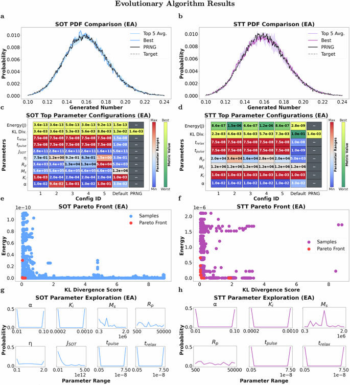
a, b PDF comparison of top 5 device configurations, best configuration, pseudo-random number generator (PRNG), and target distribution for both SOT and STT devices. c, d Parameter configurations of top 5 devices with energy and Kullback-Leibler (KL) divergence metrics compared against the default configurations and a PRNG for both SOT and STT devices. e, f Pareto fronts comparing energy and KL divergence metrics of various SOT and STT device configurations. g, h Probability distributions of the parameter ranges that were explored for both SOT and STT devices.
Figure 5c, d show the top 5 device configurations discovered across EA runs along with their KL divergence and energy metrics for the SOT and STT devices, respectively. These are compared against the default configurations and PRNG. Similar to the RL results, these configurations were also able to outperform the default configurations in terms of KL divergence. However, the energy metric is relatively close to the default configuration for the SOT device, except for the STT device, where the optimized configurations had better KL divergence scores at the expense of increased energy consumption compared to the default configuration. Additionally, the device configurations are much more similar to each other, with consistent values discovered for trelax, tpulse, and α across a majority of the best configurations for both device sets. This is most prominently seen in the STT device, where most of the variation occurs in the Rp parameter. The parameter values also tend to be closer to the bounds of the respective ranges except for the Rp parameters for STT and the η parameter for SOT.
Figure 5e, f depict the Pareto fronts for the multi-objective EA, comparing energy consumption and KL divergence of the valid configurations for both SOT and STT devices, respectively. We can see that there are a variety of device types that are explored across the performance space for both SOT and STT. These figures once again show that there are many configurations that use less energy but have high KL divergence. Unlike the RL results, Fig. 5f shows more exploration in the STT space. This plot shows that the EA likely explored two distinct local optima in the search space at two different energy levels (one higher and one lower) with varying levels of KL divergence. However, well-performing (low KL divergence and low energy) device configurations were still discovered. Similar to RL, there are fewer valid configurations for the STT device, which further supports the idea that there is a smaller subset of valid configurations for this device type.
Figure 5g, h show the probability distributions of the parameter ranges that were explored through the EA approach for both SOT and STT devices, respectively. We can see in these plots that only the extremes in the parameter range are explored for some parameter sets like α, tpulse, trelax, and Ki. This is consistent with what we saw for those parameter values in the RL approach as well. However, while the RL approach kept to the extremes for all of the device parameter values, the EA explores across the ranges for some of the device parameters, in particular Ms and Rp. We can confirm in Fig. 5c, d that the best-performing configurations for Rp and Ms tended to fall more toward the middle of the available parameter range, rather than at one of the two extremes.
Discussion
The key contribution of this work is the complete device codesign framework for true random number generation based on abstract device models for EA and RL approaches, which is illustrated in Fig. 1. The creation of such a framework requires device expertise, AI expertise, and application expertise. However, now that the framework and components have been established, it is worth noting that though we have showcased results for EA- and RL-based automated codesign approaches, SOT and STT-MTJ devices, and gamma distributions, we can easily extend this work in the future by augmenting or swapping out components within the framework. First, we can investigate other design or optimization approaches for the device parameters, such as particle swarm optimization or generative AI. Next, we can swap out or augment the MTJ devices with other probabilistic devices. Finally, we can use the framework to pick materials and device parameters for other non-uniform distributions or target codesign for other application domains.
Our second contribution is the demonstration of codesigned materials and device parameters for both SOT and STT-MTJ devices for efficient random number generation and thus, new candidate devices. It is important to note that though the default parameter values for both the SOT and STT devices are very similar, both RL and EA approaches discovered parameter sets that were clearly different for each of the two devices. This clearly indicates that leveraging an automated optimization approach for discovering device parameters is worthwhile for these sets of devices. Specifically, by leveraging an optimization approach for each individual device type and application combination, device parameter sets can be discovered that improve performance over the defaults for a particular application, while also tuning the parameters to incentivize certain metrics such as energy efficiency. In this work, the parameter ranges were kept in ranges realistically achievable in the CoFeB–MgO system through materials engineering; future work could expand the ranges further to explore not yet discovered systems.
The last main contribution of this work is the comparison of RL and EA approaches for device design. In comparing these two approaches, there are several points worth noting. First, the EA approach we used, NSGA-II, is particularly focused on multi-objective optimization and exploration of points along the Pareto front, whereas we used a reward function that weighted the objectives into a single score for the RL approach. It is worth noting that although multi-objective approaches exist for RL43, they are less popularly used than EA algorithms such as NSGA-II, which is why we focused on a weighted reward function for RL here. However, determining the appropriate weights for a multi-objective weighted reward function is non-trivial and often requires trial-and-error to determine the best weights for each objective.
We observe that both EA and RL explored configurations across the Pareto fronts; however, the EA approach explored the parameter search space to a larger degree, while the RL approach tended to stay toward the extremes. It is worth noting that this can be at least partially attributed to the smaller number of training timesteps (6000) for the RL approach compared to the EA approach (50 population size*50 generations*25 runs = 62, 500 timesteps). This disparity between the number of training timesteps for the two approaches was due to time and computing constraints; therefore, we would like to revisit this point in the future to compare the two approaches with similar training times. However, even with a smaller number of training timesteps, the RL approach was able to produce more unique configurations in its top-performing candidates compared to the EA approach as demonstrated by Figs. 4c, d and 5c, d. Another observation is that both optimization strategies resulted in the STT device configurations displaying larger variations in their PDFs compared to the SOT device. This, once again, suggests that the STT device has a smaller subset of valid configurations and may be more sensitive to the parameter configurations. Overall, both RL and EA approaches have clear advantages and disadvantages.
We summarize the Ku (Ku = Ki/tf, where tf is the free-layer thickness) and Ms pairs found by each approach for each device in Fig. 6. To orient the configurations within the plot, we derive a simple relationship between Ku and Ms to achieve PMA. Considering only the anisotropy energy density, the total effective anisotropy can be written as
If Keff > 0, the device will exhibit stronger PMA behavior, while if Keff < 0 the PMA will weaken (and eventually become IMA). When Keff = 0, we can define a “border” by ({K}_{{{{rm{u}}}}}=frac{{mu }_{0}{M}_{{mbox{s}},}^{2}}{2}); this line is shown in black in Fig. 6a. Looking at the regions inhabited by each device, the STT devices remain relatively close to the border, while the SOT devices favor stronger PMA. This is likely because a strong PMA is critical for the SOT device to return to a ± z magnetization state during relaxation. Example bitstreams generated by SOT devices found via the RL and EA approaches are shown in Fig. 6b, c, showing the expected SOT behavior. For most SOT devices in the configurations list the bitstreams exhibit this desired functionality, however, it is noted that occasionally the optimization strategies cause the SOT devices to operate in a stochastic regime instead, including the top discovered configurations; see Supplementary Note 2 for more information. Further, the top STT device bitstreams in Fig. 6d, e look as expected, stochastically switching to + z with an application of the STT current. Finally, it is noted that the tendency of both approaches to minimize α is likely related to the critical current required to drive MTJ switching; in ref. 44, it was shown that the critical switching current depends proportionally on α, and thus a smaller α allows for switching to occur at lower current densities.
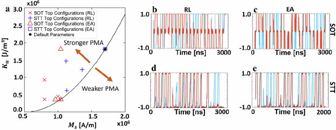
a The saturation magnetization (Ms) and volume anisotropy energy density (Ku) pairs for the top five configurations of each of the spin–orbit torque (SOT) and spin transfer torque (STT) devices found via reinforcement learning (RL) and evolutionary algorithm (EA) approaches. The SOT and STT devices generally favor configurations that have stronger perpendicular magnetic anisotropy (PMA), though the SOT devices favor weaker Ms than the STT devices. (b, c) Sample bitstreams generated using the top SOT configuration found by RL and EA approaches. d, e Sample bitstreams generated using the top STT configuration found by RL and EA approaches.
Conclusions
In this work, we proposed an AI-guided codesign framework to optimize SOT-MTJ and STT-MTJ devices for a TRNG application by utilizing RL and EA. We successfully motivated such a framework by producing valid device configurations that closely match the target distribution while optimizing for energy efficiency. We also demonstrate the feasibility of swapping components of the workflow to fit application requirements by switching out different device types (SOT vs. STT) and design/optimization strategies (RL vs. EA). We found that by optimizing the parameters of the devices beyond their default values, we can tune the MTJ devices to more closely mimic the desired distribution while simultaneously minimizing energy usage, demonstrating that using optimization-guided codesign approaches can discover or optimize devices for particular applications.
As noted previously, we intend to use this framework to tune the parameters of additional probabilistic device types, such as tunnel diodes and other types of MTJs, as well as investigate generating samples from other probability distributions beyond exponential and gamma. Additionally, we plan to continue investigating other approaches for material and device parameter search, such as particle swarm optimization, to further understand what the tradeoffs are for each optimization approach. Finally, we also plan to extend to circuit and system design while codesigning the devices for various application types, providing a full-stack optimization paradigm.


Responses