An advanced light scattering apparatus for investigating soft matter onboard the International Space Station

Introduction
Condensed soft matter systems consist of objects with sizes in the nanometer to several micrometers range suspended in a fluid, most often water. While the nature of the individual objects may vary, from solid colloidal particles to liquid droplets, surfactant molecules, polymers and proteins, and even cells and their constituents, soft systems share common features, such as the relevance of Brownian motion and the high susceptibility to external fields, even of modest strength, which originated the very term ‘soft matter’1. Soft systems are ubiquitous in everyday products and industry and are often investigated as model systems for their atomic or molecular condensed matter counterparts. Current challenges in soft matter include understanding and rationalizing out-of-equilibrium phenomena and addressing disorder and the existence of a hierarchy of length scales, due to the organization of the individual constituents in superstructures, e.g., in crystallization or gelation, or by self-assembly2.
While gravitational forces are rarely relevant at the single object scale, they do play a major role when, e.g., colloids or proteins assemble to form large structures, which may rapidly settle, or through which gravitational stress may be transmitted and accumulated over macroscopic distances. For some systems, the effect of gravity may be mitigated by matching the density of the background fluid to that of the suspended objects; however, buoyancy matching may be unfeasible without changing significantly the physicochemical properties of the system, or while concomitantly achieving near-refractive index matching, required for optical observations. Furthermore, shear forces due to convective currents are practically unavoidable in terrestrial gravity and can significantly impact growth processes. Soft systems are thus natural candidates for microgravity research3 and have been extensively studied in experiments in sounding rockets, or onboard the Space Shuttle and the International Space Station (ISS). Crystallization experiments on macromolecules4, proteins5,6,7,8, drugs9, and colloids10,11,12 have allowed for the characterization of growth rates and the obtention of crystals of larger size and better quality than on Earth. They have also unveiled unforeseen features, such as the dendritic growth of colloidal crystals11 and the emergence of crystalline order in dense colloidal suspensions that formed glasses in terrestrial gravity10. Colloidal gels have been investigated as prototypical network formers, unveiling slow restructuring13 and pointing to the role of gravity in limiting the growth of the fractal aggregates that ultimately form the gel14. In closely related fields, gravity has been shown to deeply affect the behavior of nonequilibrium fluctuations in complex fluids15, the stability of foams16, and the behavior of granular matter17,18, and synthetic and biological active matter19,20.
Optical methods are powerful and convenient tools to probe the structure and dynamics of soft matter. They are non-invasive and can be implemented in compact, lightweight apparatuses suitable for space flights, with designs based on low-magnification imaging and microscopy, see, e.g.,21 and references therein, holography22, shadowgraphy23, and light scattering24,25 and differential dynamic microscopy26,27. Here, we describe COLIS, an advanced light scattering-based space instrument developed for the European Space Agency (ESA) Colloidal Solids project, aiming at investigating onboard the ISS the origin, formation and dynamics of colloidal and protein crystals, and colloidal glasses and gels, in a series of campaigns to start in spring 2025. COLIS enables in-situ monitoring of the dynamics of physical processes during and after solidification, which is needed to assess the role played by gravity on the properties of growing structures, addressing long-standing questions such as the effect of gravity on protein nucleation28 and on anomalous, ultraslow and heterogeneous relaxations in gels and glasses29,30,31. COLIS features an unprecedented combination of light scattering techniques that can be used simultaneously: conventional dynamic light scattering (DLS)32 at three angles, paired, at the same angles, by photon correlation imaging (PCI)33, a method that blends scattering and imaging to probe heterogeneous dynamics; small-angle static and dynamic light scattering leveraging the multispeckle method34 to address slow, non-ergodic dynamics, as in gels and glasses, and absorbance measurements. All scattering detectors are equipped with a polarizer, allowing for both conventional polarized light scattering and depolarized scattering, e.g., for probing rotational dynamics of optically anisotropic samples. Finally, COLIS affords advanced sample environment controls: fluid stirring, accurate temperature control including the possibility of performing fast T jumps, and local heating of the scattering volume through a near-infrared auxiliary laser beam, for the optical manipulation of thermosensitive samples35.
Results
The COLIS setup
COLIS is designed to be operated on board of the International Space Station (ISS), accommodated inside the Microgravity Science Glovebox (MSG) host facility. It is comprised of the following main diagnostics, shown schematically in Fig. 1 (see the Supplementary Information for details on the optical design and the hardware):
-
A power-adjustable polarized (max 150 mW) optical green laser (wavelength 532 nm) equipped with a shutter.
-
A near infrared (NIR) laser (wavelength 975 nm) coaxial to the green laser, to dynamically heat water-based solutions. The laser intensity can be easily modulated, e.g., cyclically.
-
Three Dynamic Light Scattering lines, at forward, 90° and backscattering angles, denoted by DLS45, DLS90, and DLS170 in the following. The scattered light is collected by collimated single mode fibers, all equipped with a rotating linear polarizer and connected to photon counters and hardware correlators.
-
Three Photon Correlation Imaging lines (PCI45, PCI90, PCI170), at the same scattering angles as the DLS lines, and all equipped with rotating linear polarizers. For each PCI line, the scattered light is imaged on a temperature-stabilized CMOS camera for multispeckle analysis.
-
A small angle light scattering (SALS) setup, equipped with a beam block and a rotating linear polarizer. Scattered light at angles in the range 0.5°–9° is recorded by a temperature-stabilized CMOS camera.

Top panel: Experimental unit showing the optical diagnostic lines. Light green: optical path of the green laser (λ0 = 532 nm); dark green: paths of the scattered light collected by the optical diagnostic of the instrument; dark red: near infrared laser (λ0 = 975 nm). The NIR and optical beams are colinear; here they have been slightly offset for clarity. Bottom panel; section of the cell module E, indicating the optical accesses for the various diagnostic.
COLIS adopts a modular design concept similar to the SODI experiment23. It comprises three modules that will be separately uploaded in soft stowage bags and then integrated in the MSG by the ISS crew:
-
Experiment unit (EU), top of Fig. 1. The EU contains all the optical sub-systems needed for the scattered light diagnostics (DLS, PCI, SALS). Its main function is the acquisition of the scientific data.
-
Cell module (CM), bottom of Fig. 1. The CM contains the actual sample and can be inserted in a slot of the EU. The CM provides two levels of containment for the experiment liquid, the third one being that of the EU. The CM contains all the necessary hardware for the sample environment (stirring mechanism, Peltier elements, pressure compensator, etc.). For each new experiment, a separate CM is uploaded and inserted into the EU by the ISS crew.
-
Image processing unit (IPU). All the power and data lines of the MSG are connected to the IPU, which houses a powerful computer, that fulfils functions such as communicating with the outside world, controlling the experiment timeline and parameters, commanding the thermal control and sample stirring, pre-processing the PCI ans SALS images to reduce the amount of data to be downlinked to ground. These functionalities allow for quasi-autonomous operation for prolonged period of times, up to several days, and for uplinking new experimental protocols to fit future science needs. Two data disks are uploaded as part of the IPU. They are used to store the raw and pre-processed scientific data and can be exchanged on the ISS, if needed. They can be returned to ground, for further in-depth analysis of the raw data.
Overview of the experimental unit
Optical laser source
The optical laser source is a continuous–wave diode–pumped laser operating at a fixed in-vacuo wavelength λ0 = 532 nm. The laser head is pigtailed and the the maximum beam power is ≥170 mW at the fiber exit and ≥150 mW on the sample. A collimator at the fiber exit generates a collimated beam with a diameter of 1.5 mm ± 0.1 mm (at 1/e2), with a divergence angle of 0.01° ± 0.02°. A laser shutter and attenuator allows for controlling the sample illumination. In case of shutter failure, an ISS crew member can manually set the shutter in the (permanently) open position. For monitoring purposes, a beam sampler is used to redirect a small fraction ≈1% of the laser beam to a low-noise photodiode.
Near infrared laser source
The NIR laser is a fiber-Bragg-grating and thermally-stabilized laser diode operating at λ0 = 975 nm, with a maximum power of 500 mW. The laser intensity is monitored by an internal photodiode. A collimator generates a collimated beam with a diameter of 2.10 mm ± 0.11 mm (at 1/e2) with a divergence angle of 0.017°. The NIR beam is coaxial to the green laser beam, so as to heat the scattering volume. After passing through the sample, the NIR beam is stopped by the SALS beam block.
Dynamic light scattering lines
For DLS, pick-up fibers collect light scattered at three angles, whose values in air, with respect to the incident beam direction, are 45°, 90°, and 166.65°. The corresponding scattering angles θ in the sample depend on the solvent refractive index, due to refraction effects. They can be calculated using Snell’s law, considering simply a solvent-air interface, since the cell glass windows are parallel slabs that do not change the propagation direction. For water-based samples, using ({n}_{{H}_{2}O}=1.33), one obtains θ = 32.12°, 90°, and 170°, respectively.
Each collecting fiber is equipped with its own polarizer (polarization extinction ratio > 10,000:1), to perform polarized and depolarized light scattering. The scattered light collected by the fibers is fed to three avalanche photodiodes, connected to hardware correlators, for real-time calculations of the intensity correlation function for delay times from 12.5 ns to about 1 h.
Photon correlation imaging lines
Each PCI line comprises optics that image the scattering volume, as seen from one of the three angles defined above for DLS, on a USB3.0 CMOS camera, see Fig. 2 for typical PCI images. The PCI cameras have a resolution of 2048 × 1536 pixels and a pixel size of 3.45 μm (sensor size: 7.1 mm × 5.3 mm). At 8-bit, the resolution used in COLIS, each camera has a maximum full-frame acquisition rate of 120 Hz. The frame rate may be increased by decreasing the number of acquired pixel rows. For example, in order to image the full scattering volume the PCI90 camera is run at 2048 × 640 pixels, corresponding to a field of view of 5.1 mm × 1.6 mm. Under this condition, the acquisition rate is up to 287 Hz. Each camera is cooled to the working temperature, using a Peltier module (camera housing temperature Th = 38 ± 0.02 °C). The imaging optics comprises an objective lens and a circular diaphragm placed in its focal plane. The purpose of the diaphragm is to control the size of the speckles formed on the CMOS detector (about 3 pixels), and to guarantee that the scattering angle and magnification of the light rays reaching the detector are uniform across the detector area (telecentric conditions). A magnification of 1.38 is chosen, resulting in a full-frame field of view of 5.1 mm × 3.8 mm.
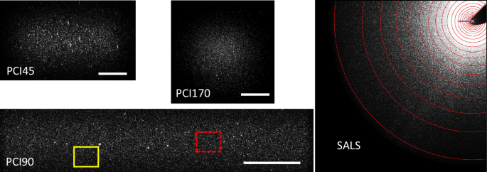
The PCI images have been cropped to show only the scattering volume; the bar corresponds to 1 mm. Different ROIs in the PCI images, such as the two boxes shown for PCI90, correspond to distinct regions of the scattering volume, but to the same scattering angle. For the SALS camera, each annular ROI corresponds to light scattered by the whole illuminated sample within a narrow range of scattering angles. The beam block that stops the transmitted beam is visible in the top-right corner, the cross indicates the position of the transmitted beam, and the blue bar corresponds to a scattering angle θ = 1°. Pixels masked by the beam block are excluded from the annular ROIs. See Section “Small-angle light scattering” for details on how the large variation of the scattered intensity with θ is dealt with, to avoid over- or under-exposing the image.
Small angle light scattering line
The optical path of SALS may be divided into two parts: right after the cell module, a Fourier lens generates a far-field scattering pattern in its focal plane, where a beam block redirects the unscattered beam to a photodiode, for absorbance measurements. The beam block can be translated along two orthogonal directions in the focal plane, to optimize its positioning. The second part is composed of a relay lens that forms an image of the plane of the beam block on the sensor of the SALS camera. The SALS optics is designed to collect light scattered at angles θ ≤ 9°. The speckle size is slightly angle-dependent, ranging from 2 to 5 pixels. The SALS line is equipped with a USB3.0 camera mounted on a Peltier cooler. A CMOS detector is used to avoid blooming (overflow of photo-induced charge carriers between adjacent pixels), which is particularly important for small angle measurements, where the scattered intensity may vary over several orders of magnitude over the detector area. The sensor has 2048 × 2048 pixels, with a pixel size of 5.5 μm. A polarizer (extinction rate ≥ 10,000:1) is placed behind the beam block. The polarizer can be rotated continuously in order to further control, for non-polarizing samples, the light intensity that reaches the camera, or to perform depolarized light scattering.
Sources and image acquisition synchronization
A TTL pulse generator with time resolution of 0.1 ms is used to control the timing of the image acquisition of the PCI and SALS cameras, the status of the NIR laser (ON/OFF) and the operation of the optical laser shutter. A trigger pattern usually lasting a few tens of seconds and comprising hundreds of image acquisitions is typically repeated cyclically, for an overall measurement duration up to tens of hours. The pulse generator guarantees that the camera images are taken sequentially, to avoid bus conflicts, and that the shutter is open while acquiring images. It is also used to illuminate cyclically the sample with the NIR beam, to create a periodic thermal perturbation.
Cell module
The cell module (CM) of COLIS is an exchangeable unit that contains the experiment fluid and all the hardware for thermal control and sample stirring, see Fig. 1. The CM provides:
-
Optical access for the optical and NIR laser beams and for all scattered light measurement lines.
-
Control and monitoring of the cell temperature.
-
Two levels of containment of the experiment fluid, through the sample optical cell in the center of the CM and the six CM windows.
-
Stirring of the experiment fluid through a magnetic bar placed in the cell and actuated by a rotating magnet placed below the cell.
Two different types of Cell Modules are designed: CM E and D.
Cell module E
The CM E is designed to ensure low thermal gradients and high stability of the experiment fluid, to allow for experiments lasting up to several days at a fixed temperature. Its thermal inertia is still low enough to allow for imposing several kinds of thermal histories, such as temperature jumps (for example upward T jump of 5 °C with a rate up to 5 °C/min), ramps, and periodic temperature oscillations (e.g., a nearly sinusoidal T oscillation with period 60 s and peak-to-peak amplitude of 2 °C). The sample temperature is monitored by 3 thermistors placed in thermal contact with the outside walls of the optical sample cell. The inner dimensions of the optical cell in the scattering plane (the plane of Fig. 1) are: 5 mm along the direction of the optical axis, 9 mm in the direction orthogonal to the optical axis, to accomodate the DLS45 and PCI45 lines. The inner height of the cell is 7 mm. The stirring system imposes the rotation of a magnetic bar located in the bottom part of the sample cell, see Fig. S35 of the Supplementary Information, at up to 5000 rpm in both directions. It applies a torque sufficient to transmit shear forces to the whole sample volume, thereby fully homogenizing fluids with a viscosity up to 100 mPa s (100 times the water viscosity) and a yield stress up to 5 Pa, in 30 min or less.
Cell module D
Cell module D is designed primarily for protein solution experiments, where the amount of sample is usually quite limited, thermal requirements are stringent, and only DLS90 and absorbance measurements are needed. These features are accounted for by using an optical cell with a reduced sample volume of 0.1 ml, less than one-third of that of CM E, and by suppressing the unused CM windows. The thermal gradient and thermal stability thus obtained are <0.05 °C/cm over the cell (in all directions), and <0.03 °C over 10 h, respectively. Furthermore, CM D allows for quenching temperature from 25 °C to 10 °C in less than 30 s, in order to trigger protein nucleation at a well-defined time. In addition to the gradient, stability and T ramp requirements, it is also required to increase/decrease the temperature in the range of 10–40 °C. The stirring and temperature monitoring systems are very similar to those of CM E.
Scattering methods
We briefly introduce the main features of the static and dynamic light scattering methods implemented in COLIS.
Dynamic light scattering
Dynamic light scattering is a well-established method to probe the dynamics of soft matter systems32 on time scales ranging from 10 ns to about 100 s, and on length scales in the range 1 nm to about 1 μm, depending on the experimental geometry. In the COLIS implementation of DLS, the sample is illuminated by the optical laser beam with in-vacuo wave length λ0 = 532 nm and light scattered at the three scattering angles mentioned in Section “Overview of the experimental unit” is collected by fiber optics and fed to fast, sensitive avalanche photodiode detectors. The information on the sample dynamics is encoded in the temporal fluctuations of the scattered intensity, I(q, t), which are quantified by the time autocorrelation function
where (q=4pi n{lambda }_{0}^{-1}sin (theta /2)) is the modulus of the scattering vector, n the refractive index of the solvent, θ the scattering angle, and < … > t indicates a time average. Note that here we have assumed that the system is isotropic, such that g2 − 1 does not depend on the orientation of the scattering vector. The intensity correlation function is related to the field correlation function g1, also known as intermediate scattering function, by the Siegert relation:32
where the coherence factor α is a setup-dependent constant32, close to 1 for COLIS. In the last equality of Eq. (2), the term in the brackets is the (collective) intermediate scattering function f(q, τ), where we have assumed for simplicity that the scattering is due to N identical particles, with time-dependent positions r1, . . . , rN, and that the system is ergodic and the dynamics stationary, such that the ensemble average < … > in Eq. (2) is equivalent to the time average used to calculate g2 − 1.
COLIS allows for both polarized and depolarized DLS, thanks to polarizers placed in front of each DLS fiber optic. The conventional ‘polarized’ DLS configuration, or VV configuration, is obtained by orienting the polarizers’ transmission axis in the same direction as the polarization direction of the incoming beam. ‘Depolarized’ dynamic light scattering (DDLS) corresponds to the so-called VH geometry, where the polarizers’ axis is rotated by 90 degrees with respect to the incoming beam polarization. For optically isotropic particles, the VH component of the scattered intensity is zero. By contrast, the scattered intensity from either geometrically or optically anisotropic particles has both a VV and a VH component. We recall here only a few results for DDLS from partially crystalline colloidal particles, of interest for the experiments discussed in Section “Depolarized DLS”, see ref. 36,37 for a more detailed discussion. A DDLS experiment measures ({g}_{2}^{VH}(q,tau )-1), the autocorrelation function of the depolarized scattered intensity. Assuming that the orientation of the optical axis of distinct particles is uncorrelated and that the particle orientation and translation are decoupled, one finds:
where fs(q, t) is the translational self intermediate scattering function and fr(t) is its (q-independent) rotational counterpart. Thus, under the conditions mentioned above, DDLS differs from DLS in two important respects: it probes self rather than collective dynamics, and it is sensitive to both translational and rotational dynamics.
Space- and time-resolved dynamic light scattering: photon correlation imaging
Soft solids such as gels and colloidal glasses often exhibit relaxation times as long as several hours and heterogeneous dynamics that evolve and fluctuate both in time and spatially. Conventional DLS can not cope with these features, because it relies on extensive time-averaging, which should typically last 103–104 times longer than the longest relaxation time of the system32, and because the scattered intensity collected by the detector originates from the whole scattering volume. Photon Correlation Imaging33 is a multispeckle technique38 that overcomes these limitations by using CMOS cameras as detectors and by combining scattering and imaging. In COLIS, three PCI cameras make an image of the scattering volume, using light scattered approximately at the same angles as for conventional DLS. Due to the coherence of the illuminating beam, the small acceptance angle of the objective lenses used to form the image (3. 1° for water-based samples, as set by a diaphragm placed in the focal plane of the objective lens), and the low magnification (M = 1.38), individual colloidal particles cannot be resolved in the PCI images. Rather, the images have a speckled appearance, as shown in Fig. 2. Distinct regions of interest (ROIs), such as the two boxes shown in the PCI 90 image, correspond to distinct regions within the scattering volume. Accordingly, the dynamics are quantified by a space- and time-resolved degree of correlation cI:
where Ip is the intensity measured by the pth pixel, < … > p∈ROI(r) indicates an average over pixels p belonging to a ROI centered around position r in the sample, and where the normalization introduced in the second line results in cI(τ = 0) = 1 and reduces the statistical noise associated to the finite number of pixels for τ > 039. For stationary, spatially uniform dynamics, averaging cI over t and r yields the conventional g2 − 1 function of Eq. (1). Note that CMOS cameras typically have non-negligible dark counts. Therefore, Ip in Eq. (4) is obtained by subtracting a dark background from the CMOS signal, as detailed in39. All calculations required to obtain cI are performed on-board, using a dedicated, in-house software. The software allows also for correcting cI for any rigid drift of the speckle pattern within a ROI40, which may occur in gels or glasses due to the relaxation of internal stresses.
Small-angle light scattering
Small angle light scattering (SALS) is implemented in COLIS using a CMOS camera, allowing for both static and dynamic light scattering measurements. The optical layout is similar to that of ref. 41: light scattered at small angles (typically, 0.25° ≤ θ ≤ 10°, corresponding to more than a decade and a half in scattering vector magnitude, 0.06 μm−1 ≤ q ≤ 2.7 μm−1) is collected by a Fourier lens; an objective lens images the focal plane of the Fourier lens onto the CMOS sensor. A typical SALS image is shown in Fig. 2. The transmitted beam is stopped by a beam block, placed in the focal plane of the Fourier lens; pixels at a distance rp from the transmitted beam position receive light exiting the cell at an angle (arctan ({r}_{p}/{f}_{eff})), where feff = 38.18 mm is the effective focal length of the SALS apparatus, which accounts for both the focal length of the Fourier lens and the magnification of the objective lens.
As seen in Fig. 2, the SALS scattered intensity usually varies considerably with θ, making it impossible to correctly capture I(q) over the full range of SALS q vectors using a single exposure time. To circumvent this problem, a burst of images at a predefined set of exposure times is acquired and a single composite image is reconstructed using, for each ROI, the data collected at the optimum exposure time. The ROIs have an annular shape, corresponding to a small range Δθ of scattering angles centered around a well defined θ, with Δθ/θ ≲ 0.1, and the optimum exposure time is chosen such that the ROI-averaged intensity is closest to, yet smaller than, an empirically determined threshold of 40 gray levels for 8-bit images, as detailed in ref. 42. As for PCI, a dark background is subtracted systematically before further processing of the images.
The composite images are used for both dynamic and static SALS. For dynamic light scattering, the images are processed in the same way as PCI images, Section “Space and time-resolved dynamic light scattering: photon correlation imaging”, the only difference being that all averages are performed on the annular ROIs, yielding one cI(q, t, τ) dataset per ROI. Note that there is no r dependence in the SALS cI: SALS data are collected in the far field geometry and thus lack spatial resolution, in the sense that each pixel receives light from the whole scattering volume. It is worth mentioning that the → 0 limit of cI(q, t, τ) depends in general on the exposure time43. Hence, care should be taken in comparing data acquired at different q vectors. Using the normalization scheme of the second line of Eq. (4) helps mitigating this issue.
Static SALS is performed by calculating the intensity of the scattered light averaged over all pixels belonging to a given ROI and by applying several normalization factors:
where < … > q indicates the average over all pixels belonging to the annular ROI associated to a scattering vector of magnitude q, Ip,opt(t) in the r.h.s. refers to the intensity measured at the optimum exposure time, Eopt(q, t) is the time- and q-dependent chosen optimum exposure time and Eref is an arbitrary reference exposure time, set to 1 ms in COLIS. The normalization factor C(q) accounts for the small variation of the solid angle associated with each pixel (less than 10% over the angular range of COLIS, see ref. 42 for details), and PDT(t) is the intensity of the incident beam at the time of the acquisition, obtained from the monitor photodiode mentioned in Section “Overview of the experimental unit”. Although no absolute intensity calibration is available in COLIS, the normalization factors included in Eq. (5) allow for comparing the relative intensity between different samples.
Small angle scattering is notoriously challenging because any imperfection in the optical elements (lenses, cell walls, additional windows introduced to meet safety rules imposing multiple containment levels, etc.) scatters light in the SALS angular range. Correction schemes for this so-called optical background are possible for both dynamic34 and static measurements42, provided that one can measure the scattering pattern with the cell filled with only the solvent, using the very same cell that will be later loaded with the sample. Because COLIS is designed to operate with various cells, some of which will not be available prior to the upload of the setup onboard the ISS, these correction schemes will not always be applicable. Examples of SALS data with and without optical background correction will be presented in Section “Small-angle static and dynamic light scattering”.
In the following, we illustrate most of the capabilities of COLIS, starting from validation tests on model colloidal particles and then move to more complex protein, gel, and glassy systems.
Brownian dynamics of model colloidal particles
Polarized DLS
We test VV, or polarized, dynamic light scattering at the three wide angles covered by COLIS by measuring the Brownian dynamics of a diluted suspension of polystyrene (PS) particles, using both the avalanche photodiode detectors and hardware correlators (DLS, hereafter) and the PCI cameras. For the latter, we use the variable delay acquisition scheme of ref. 44, which allows probing τ delays as small as 2 ms while keeping low the average image acquisition rate (here, 2 Hz). All measurements are performed simultaneously (Fig. 3a) shows data for the PCI 90° camera, for three successive runs, showing excellent repeatability. The intensity correlation function, obtained by averaging cI over the full scattering volume and over time, is fitted by (line in Fig. 3a):
where for Brownian particles the relaxation time reads ({tau }_{r}={(D{q}^{2})}^{-1})32, with D the (translational) diffusion coefficient given by the Stokes–Einstein relation, D = kBT/(6πηR), with R the particle radius R, η the solvent viscosity, T the absolute temperature and kB Boltzmann’s constant. A ≲ 1 is a constant that depends on the speckle-to-pixel size ratio45 and B ≈ 0 is the baseline39. Note that, since CMOS cameras are slower detectors compared to the avalanche photodiodes used for DLS, the smallest delay time τ accessible by PCI is here 5 ms, still sufficient to correctly capture the particles’ dynamics.
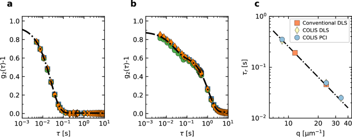
a Intensity correlation function measured by the PCI90 camera. Symbols: data from three independent runs; line: fit with Eq. (6). b same as in (a), for θ = 170.8°. The line is a double exponential fit, Eq. (7), to account for the observed two-step decay, which is due to a partial reflection of the incoming laser beam on the exit wall of the cell, see text for details. c Fitted relaxation time as obtained by COLIS (PCI and DLS detectors) and by a conventional setup, as a function of scattering vector q. The line is a fit to the data using the power law τr ∝ q−2 predicted for Brownian translational diffusion. Error bars, as obtained from the fit, are smaller than the symbol size.
A similar exponential relaxation is seen for the DLS data at θ = 90° and for both the PCI and DLS data at nominal 45° (θ = 29.32°, see Fig. S42 of SI). By contrast, the correlation function measured at θ = 170.8° exhibits a surprising two step decay, Fig. 3b. This behavior is reminiscent of that reported in ref. 46. It is due to the reflection of part of the incident beam at the cell exit wall, an effect already discussed in the early light scattering literature47. This reflected light propagates backward in the scattering cell, along the same axis as for the incident beam, but in the opposite direction. As a result, the detector at θ = 170.8° collects both backscattered light and light scattered in the forward direction by particles illuminated by the counter-propagating reflected beam. The intensity correlation function can then be modeled by the squared sum of two exponential relaxations, corresponding to the two contributions (line in Fig. 3b); further assuming Brownian dynamics, leads to
where the indexes f and b refer to forward- and back-scattering, respectively.
Figure 3c shows the q dependence of the relaxation time ({tau }_{r}={(D{q}^{2})}^{-1}) obtained from the fits of g2 − 1 (Eq. (6) for data at θ = 29.32 and 90°, backscattering term of Eq. (7) for the data at θ = 170.8). Additional measurement performed on the same sample using a conventional, commercial setup (Brookhaven BI-9000AT) are also shown (red squares). All data fall onto the same straight line on a double logarithmic plot, corresponding to the q−2 scaling expected for Brownian dynamics. A power law fit to the data, τr = D−1q−2, yields D = 0.0390 ± 0.0006 μm2 s−1, in good agreement with D = 0.035 ± 0.004 μm2 s−1 as calculated using the nominal particle size and nominal solvent viscosity.
Depolarized DLS
We show data obtained for a diluted suspension in water of Brownian, non-interacting and nearly monodisperse particles made of Hyflon MFA, a copolymer of tetrafluoroethylene and perfluoromethylvinylether. Under these conditions, the expected functional form for the DLS g2 − 1 is given by Eq. (6), while for DDLS Eq. (3) reduces to
where D and Dr = kBT/(8πηR3) are the infinite-dilution translational and rotational diffusion coefficients of a single particle, respectively, and A ≲ 1 and B ≈ 0 are as in Eq. (6). Note that the relaxation of ({g}_{2}^{VH}-1) is exponential, as for DLS, but with a modified decay rate (Gamma equiv {tau }_{r}^{-1}={q}^{2}D+6{D}_{r}).
We run simultaneous DLS measurements at T = 25 °C using the DLS45, DLS90, and DLS170 COLIS lines, which correspond to θ = 32.12°, 90.0°, and 170.0°, and q = 8.7 μm−1, 22.2 μm−1, and 31.3 μm−1, respectively. Measurements are run in both the VV and the VH configuration. Figure 4a shows the θ dependence of the intercept of the correlation functions, i.e., their τ → 0 value. For the VV component, the intercept drops sharply for backscattering, most likely due to the contribution of stray light stemming from the back reflection of the transmitted beam on the cell exit wall, as discussed in Section “Polarized DLS”. By contrast, the intercept of the depolarized correlation function exhibits only a mild θ dependence, because the crossed polarizer blocks the spurious back-reflected light, responsible for the lower VV intercept.
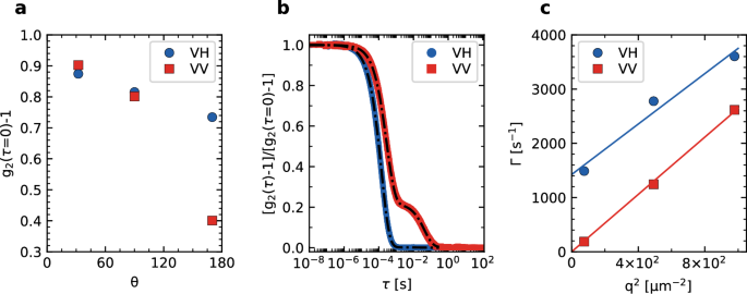
a g2(τ → 0) −1 vs scattering angle for polarized (VV, red squares) and depolarized (VH, blue circles) conditions. Error bars, as obtained from the standard deviation over four independent repetitions, are smaller than the symbol size. b VV and VH intensity correlation functions measured at θ = 170.0° with COLIS DLS170. Continuous lines are fits as discussed in the main text. c q dependence of the decay rates obtained from the fits to g2 − 1, for VV and VH conditions. Error bars, as obtained as for a, are smaller than the symbol size.
The presence of a spurious contribution in the DLS170 data, due to unwanted back-reflected light, is confirmed by inspecting the shape of g2 − 1. As shown in Fig. 4b (red squares), ({g}_{2}^{VV}(tau )-1) exhibits two distinct decay times, as already observed in the polarized DLS data of Fig. 3b, due to the back-reflection of the incident beam at the cell exit wall discussed above. By contrast, ({g}_{2}^{VH}(tau )-1) exhibits a nearly exponential decay, as predicted by Eq. (8). A careful inspection of the VH correlation function, however, reveals very small deviations from a simple exponential relaxation, which we attribute to a small fraction of VV light passing through the polarizer, due to its imperfect alignment and to the small birefringence of the optical windows and lenses. Accordingly, we fit the DDLS correlation function measured by DLS170 with the following expression:
where the first term on the right-hand side accounts for the expected DDLS VH contribution, while the second one accounts for a small residual VV component. The latter is modeled using Eq. (7), with parameters obtained by fitting the VV data shown as red squares in Fig. 4. The coefficient a accounts for the relative weight of the VV and VH components, yielding an effective extinction ratio of the polarization optics of COLIS of 0.02. Figure 4c shows the decay rate (Gamma ={tau }_{r}^{-1}) (symbols), obtained from the fits to the VV and VH correlation functions. Fitting the VV relaxation rate to Γ = Dq2 (red line in Fig. 4c) and using the Stokes–Einstein relation with η = 0.893 ± 0.002 mPa s−1 yields R = 92 ± 2 nm. The VH relaxation rate is consistent with the expected behavior Γ = 6DR + Dq2 (blue line in Fig. 4c). The particle radius may be estimated from D, yielding R = 105 ± 10 nm, or using the ratio between the translational and rotational diffusion coefficients, yielding (R=sqrt{3D/4{D}_{R}}=85pm 10) nm. By averaging the R values issued from the three methods we obtain R = 93 ± 5 nm, in good agreement with the expected value, R = 90 ± 2 nm.
Small-angle static and dynamic light scattering
Figure 5 shows static and dynamic light scattering data (SALS-SLS and SALS-DLS, respectively) obtained for diluted suspensions of colloidal particles using the SALS camera of COLIS.
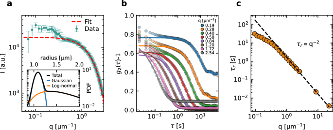
a Static scattered intensity vs q after optical background subtraction, for a diluted suspension of SiO2 colloids. Error bars are the standard deviation over a time series of scattering images. b Representative g2 − 1 functions measured with the SALS camera for a a diluted suspension of PS particles, with no optical background subtraction. c q dependence of the relaxation time of the correlation functions shown in (b), with additional data points obtained a larger angles, using the DLS45 and DLS90 COLIS measurement lines. Error-bars are calculated using the covariance matrix from the fits and are smaller than the symbols.
The SALS-SLS data for SiO2 particles shown in Fig. 5a were corrected for the optical background, taken with the cell filled with the solvent alone, see Section “Small-angle light scattering”. Data for q ≥ 0.4 μm−1 show the characteristic decrease of I(q) expected for spherical particles. At smaller q, the scattered intensity becomes more erratic and tends to be higher than expected. This behavior is typical of scattering data collected at very small q, where the optical background is comparable to or even larger than the signal due to the particles, making it difficult to fully correct for stray light. Indeed, at the smallest q the optical background for the data of Fig. 5a was more than five times larger than the particles’ contribution. The inset shows the particle size distribution obtained using Mie theory and modeling the suspension as a mixture of quasi-monodisperse spherical particles (Gaussian distribution with an adjustable mean value and fixed relative standard deviation of 5%, as provided by the manufacturer) and a log-normally distributed population of larger effective spheres, accounting for any aggregates that may be present. The fit is performed for q ≥ 0.4 μm−1; as shown by the dotted line in Fig. 5a, it reproduces very well I(q). The Gaussian distribution accounts for 85.6% of the scattered intensity and corresponds to an average particle radius of 1.09 μm, in very good agreement with the nominal one (1.005 μm). The log-normal distribution corresponds to a small amount of aggregates with effective radius 1.54 μm and moderate polydispersity (relative standard deviation: 25%).
SALS-DLS data for Brownian PS particles were collected without taking any optical background, to test the conditions of some of the space experiments, see Section “Small-angle light scattering”. Representative g2 − 1 functions measured simultaneously at various q vectors are shown in Fig. 5b. As q decreases, the decay time increases, as expected, and the baseline increasingly departs from zero, due to the contribution of the static stray light34. The fast relaxation mode seen for τ ≲ 0.1 s is possibly due to aggregates or impurities that sediment through the beam. We fit the final decay of g2 − 1 using Eq. (6) with A, B, and the relaxation time τr as the fitting parameter. The fitted relaxation time is shown in Fig. 5c as a function of q, for the SALS data and for additional DLS measurements performed on the same sample using the COLIS DLS90 and DLS45 detection lines. The SALS relaxation time agrees well with the expected behavior for q ≳ 0.5 μm−1: in this regime, the SALS and DLS relaxation times are very well fitted by ({tau }_{r}={(D{q}^{2})}^{-1}) (dotted line), with D = 0.60 ± 0.01 μm2 s−1, in excellent agreement with D = 0.59 ± 0.02 μm2 s−1 calculated from the nominal particle radius and solvent viscosity. At lower q, the relaxation time of g2 − 1 is faster than expected, possibly due to residual sedimentation or convection.
Space-resolved measures of NIR-induced heating
As a way to demonstrate both the space resolution capabilities of PCI and the local heating of the scattering volume through the NIR laser, we build a map of the local temperature upon illuminating the scattering volume with the NIR beam. We use a colloidal glass comprising pNIPAM microgel particles, a sample with two unique properties. First, convection is suppressed, because the sample is glassy, thus avoiding mixing on macroscopic length scales when the NIR laser is turned on. Second, the scattered intensity changes upon heating, because the microgels shrink48, resulting in changes of both the form factor of the particles and the structure factor of the suspension; thus, I = I(q, T). We calibrate the temperature dependence of I by acquiring data with the PCI90 camera, with no NIR beam and using the cell temperature control to vary systematically T from Tmin = 25 °C up to Tmax = 30 °C, acquiring 16 different temperature points (more details in the Supplementary Information). For each camera pixel p, a T-dependent intensity value is obtained, allowing for building a set of Ip(T) calibration curves, see the SI for full details of the procedure. Therefore, we are able to convert the intensity values with the NIR beam on to a map of the local temperature. An example is shown in Fig. 6, which displays the T map obtained with the cell temperature set to T = 25.5 °C, both before and 300 s after switching the NIR beam on, when the T field has reached a steady state. Note that the temperature increase is as high as 1 °C, with the NIR laser running at just 20% of its maximum power. A higher NIR beam intensity induces a slow drift of the overall cell temperature, due to limitations in the power of the Peltier elements.
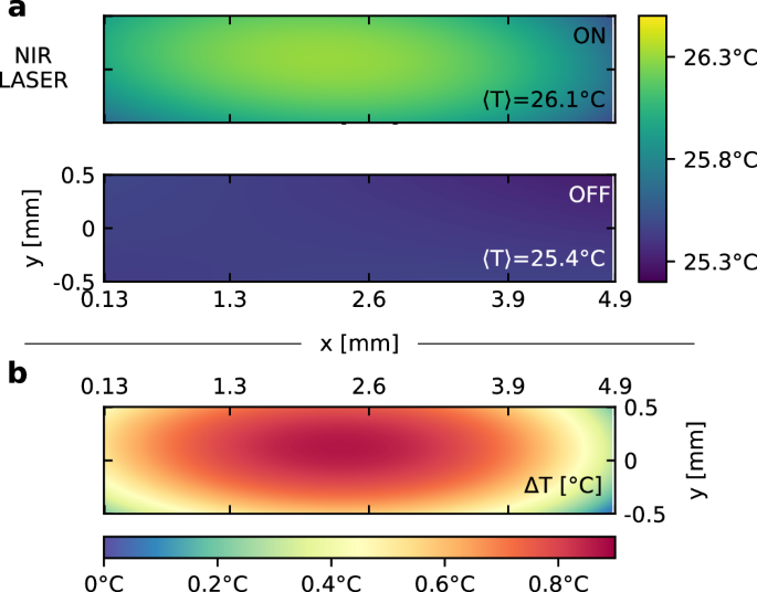
The cell temperature is controlled to T = 25.5 °C with the Peltier elements and the NIR laser is switched on during the measurement, with a power of 60 mW. a Local temperature during the “ON” and “OFF” status, respectively. The maps have been calculated averaging 180 and 20 frames for the OFF and ON status, respectively, see details in the Supplementary Information. Note the hotter region in the middle of the sample, due to the boundary conditions imposed by the Peltier elements. b Local change of T, calculated as the difference of the maps shown in panel (a).
Using COLIS to study protein nucleation
One of the planned COLIS experiments onboard the ISS is the investigation of protein nucleation, the first step of crystallization, which is a process of critical importance in the production of pharmaceuticals and in human health, as well as the object of a great deal of fundamental research. Protein nucleation frequently involves multiple steps and is affected by the presence of poorly understood protein-rich clusters thought to play a role in protein nucleation and often referred to as “nucleation precursors”49. Our experiment will make use of the unique capabilities of COLIS to very precisely control temperature and temperature changes, with a spatially uniform temperature profile (T gradients less than 0.05 °C/cm), as needed to avoid Soret effects50, while monitoring populations of clusters from molecular monomers to large precursor clusters.
Our experiments involve heating a dilute solution of proteins to 40 °C so as to dissolve any crystals present, and then to reduce the temperature to a set-point in the range of 10–15 °C as quickly as possible with minimal undershooting. The latter point is important because even if the temperature returns to the set-point, any sustained undershoot will trigger nucleation and crystal growth faster than at the set-point and, indeed, possibly too fast to monitor. Overshoots are also undesirable but do not risk making the comparison between terrestrial and microgravity experiments meaningless, as long as they are reproducible. Figure 7a shows the results of five repetitions of the cooling protocol developed in the course of ground tests. The main panel and the inset clearly demonstrate the high degree of reproducibility of the cooling curves, the rapid rate of temperature decrease (approx. 0.5 °C/s) and the very low undershoot (less than 0.015 °C).
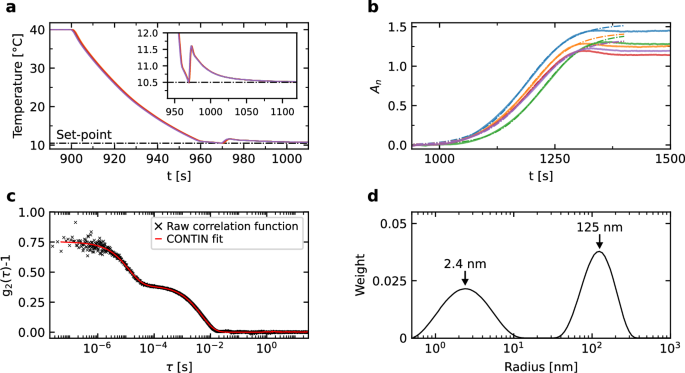
a Measured temperature as a function of time. The results of five independent runs are shown. The horizontal line at the bottom is the target final temperature. The inset shows that the undershoot is minimal. b Normalized absorbance from five repetitions of the cycle of cooling to 10.5 °C followed by heating to 40 °C. Dashed lines are fits of each curve to a sigmoid (only using data up to the maximum of each curve). c Experimental and fitted DLS correlation functions measured using DLS90 during a period of 30 s, at the end of the melting cycle at 40 °C. d distribution of cluster sizes obtained from the CONTIN fit shown in (c). The smaller peak is centered at 2.4 nm which is typical of a lysozyme molecule. The second peak, at 125 nm, is typical of the protein-rich clusters often observed prior to crystal nucleation.
The process of nucleation—that is, the formation, via thermal fluctuations, of crystalline clusters large enough to be stable and grow—will be monitored by means of DLS and absorbance. Absorbance measurements are made by measuring the intensity of the laser beam, before and after passing through the sample, I0 and It, respectively. The absorbance is defined as (A={log }_{10}({I}_{0}/{I}_{t})); in Fig. 7b we show An, the absorbance normalized by its value at time t = 0, when the proteins are fully dispersed in the solution, during one cycle of temperature reduction from 40 °C to a set-point of 10.5 °C, from our ground experiments on the protein lysozyme. The absorbance initially follows a sigmoidal curve, as expected, from which the induction time for nucleation can be extracted by fitting the data. (Only data up to the maximum of each curve is used in fits since, at later times, the curves are no longer sigmoids due to larger crystals falling out of the field of view in terrestrial gravity.) The fits show induction beginning at 285 ± 6 s after start of the temperature decrease, thus illustrating the accuracy with which the induction time can be measured from the experimental data.
The second means of monitoring the process is DLS. Figure 7c shows an example of a correlation function g2 − 1 measured using DLS90 during a period of 30 s, at the end of the melting cycle at 40 °C. Note the double shoulder in g2 − 1, which indicates at least two populations of different-sized scatterers. The data has been processed using the CONTIN51 algorithm from the Jscatter package52 and the resulting fitted signal is shown together with the experimental g2 − 1, demonstrating good agreement between the two. From this, we have information about the size and size distribution of any clusters present in the solution. For the example shown, the analysis indicates two populations of objects (Fig. 7d), one with a hydrodynamic radius of 2.4 nm, the typical size of a lysozyme molecule, and one with a mean radius of 125 nm, which is typical of the aforementioned clusters often observed prior to nucleation49.
Gelation and collapse of a physical gel
In space, COLIS will be used to investigate the slow restructuring of gels formed by attractive colloidal particles. In terrestrial gravity, the gels are unstable: they collapse or even fail to fully form due to their own weight. Here, we show how data collected with various lines of COLIS may be combined to gain a thorough picture of the impact of gravity on colloidal aggregation and gelation. In our system, a colloidal gel made of the same particles discussed in Section “Depolarized DLS” (R = 90 ± 2 nm), short-range attractive interactions between the fluorinated particles are due to depletion forces53 arising from the osmotic pressure exerted by micelles of Triton TX100, a surfactant molecule. As mentioned in Section “Materials”, the strength of these forces may be tuned by varying T, because Triton X100 exhibits an inverted consolution gap with water: due to the growth of pre-critical fluctuations of the micelle concentration, an increase in the sample temperature is associated with a strengthening of depletion effects54,55,56. We choose a sample composition such that the strength of attractive interactions steeply increases on approaching T = Tgel ≈33.5 °C, effectively triggering colloidal aggregation. Figure 8a shows the time evolution of T during a fast upward T jump. Note that, unlike the case of proteins discussed in Section “Using COLIS to study protein nucleation”, here it is not critical to avoid undershoots or overshoots of T; accordingly, the temperature control parameters were optimized for achieving a fast up-ramp, resulting in some T oscillations before reaching the target temperature of 35 °C, 1.5 °C above Tgel. The resulting absorbance normalized to its peak value, An, is shown in Fig. 8a as a solid line. An is low for T < Tgel, because the suspension is fully dispersed. As T exceeds Tgel, the absorbance strongly increases, due to the formation of colloidal aggregates driven by strong depletion interactions. Note however that An eventually decreases, for t ≳ 350 s, which is incompatible with the formation of a stable gel structure at constant T > Tgel, a first hint of gravity-induced gel disruption.
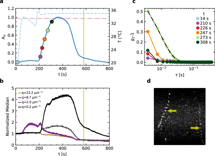
a Sample temperature (dashed line) and normalized absorbance (solid line) vs time. b Median value of the scattered intensity measured by the three PCI cameras and at one selected angle of the SALS camera, corresponding to the q values shown in the label. c Intensity correlation functions measured by PCI90 at various times t, shown as circles with the same color code in (a). d Maximum intensity projection of a burst of 15 images taken by the PCI90 camera at the time shown by the vertical lines in (a) and (b). The arrows show two trajectories of bright spots that correspond to settling colloidal aggregates.
This is confirmed by the time evolution of the median scattered intensity. Note that we use the median instead of the more common arithmetic mean, because the aggregation process results in a strong increase of the scattered light. As a consequence, a significant fraction of the camera pixels are saturated and the median is a more robust statistical estimator of the average scattered intensity. Data at representative q vectors, obtained from the COLIS cameras, are shown in Fig. 8b. The aggregation process is characterized by a strong increase in the scattered light at all angles. Previous works shows that, for colloidal aggregation resulting in fractal aggregates at fixed particle number density, the scattered intensity at any given q initially increases and then plateaus to a fixed value, see, e.g., ref. 29. Furthermore, the smaller the q vector, the longer it takes for I(q) to reach its plateau value. Both features are seen in the early stages of the time evolution shown in Fig. 8b. However, the scattered intensity eventually drops at all probed q, implying a decrease of the total number of particles in the scattering volume, presumably due to sedimentation.
To gain further insight in the aggregation process, we collect several bursts of 1000 images each, acquired with the PCI90 camera run at 275 fps. A first burst of images is taken before increasing T, when the colloids are fully dispersed. Additional bursts are triggered automatically when the absorbance level first exceeds a threshold level, set to An = 0.1, 0.3, 0.5, 0.7, 0.9, respectively (circles in Fig. 8a). The intensity correlation functions g2 − 1 calculated for each series of images are shown in Fig. 8c. Note that here the multispeckle approach afforded by PCI is essential: replacing the extensive time average required by conventional DLS with the pixel-averaging of Eq. (4) allows for following the rapidly-evolving dynamics following the onset of aggregation.
At the beginning of the aggregation process (t ≤ 210 s) the dynamics of the sample are very rapid and indistinguishable from that of the un-aggregated sample: at the minimum accessible delay, τ = 3.6 ms, g2 − 1 is close to zero. Starting from t = 226 s (An = 0.3) the dynamics steadily slow down until t = 273 s, then accelerate again, see the data for t = 308 s. The slowing down of the dynamics can be attributed to the formation of clusters of increasing size. Assuming for simplicity that the decay of g2 − 1 is due to the translational diffusion of non-interacting clusters, the typical cluster size measured at t = 273 s by fitting the data with Eq. (6) (dash-dotted line) is R = 2.42 μm, more than a factor of 25 larger than the particle size (R = 90 ± 2 nm; see “Materials” for further details). The acceleration of the dynamics at later time is consistent with the scenario of falling clusters suggested by the non-monotonic behavior of An and of the median intensity, Fig. 8a, b, respectively. Visual inspection of the PCI90 images confirms this scenario. Figure 8d shows an image obtained applying a maximum intensity projection filter (MIP) to 15 consecutive frames taken at t = 580 s (vertical line in Fig. 8a, b). Each pixel of the output MIP image is set to the maximum intensity recorded over the series of images. This allows for following the trajectory of falling clusters, which appear as bright specs in the PCI90 images, see arrows in Fig. 8d. Note that the trajectories deviate from the vertical direction due to the mixing flow in the cell induced by the falling clusters.
We emphasize that here the imaging collection optics of the PCI90 camera is essential in order to directly observe the falling clusters: had a conventional far field configuration be chosen, the speckle images would have been uniform, with no hints of the individual contribution of localized scatterers. The PCI90 images allow for rationalizing the results obtained with all other measuring lines: as the largest clusters rapidly settle to the bottom of the cell, the scattering volume is left with smaller aggregates and individual particles, leading to the decrease of An, of the median intensity and of the relaxation time of g2 − 1 (Fig. 8a–c, respectively).
Spontaneous and driven dynamics of a soft colloidal glass
We use a colloidal glass composed of thermo-sensitive pNIPAM soft microgels to demonstrate the space- and time- resolved capabilities of the COLIS setup, as well as to explore the effect of a thermal perturbation on these out-of-equilibrium samples. In colloidal systems, the glass transition is driven by particle crowding: the control parameter is the volume fraction φ occupied by the particles57. Thermosensitive colloids allow for conveniently varying φ by shrinking or swelling the particles, while working with a single sample at a fixed number density of colloids. This unique feature has made thermosensitive particles very popular; in particular, pNIPAM thermosensitive microgels are now regarded as a model system for investigating phase transitions of various kinds58, including the glass transition of soft particles31,59.
Spontaneous dynamics: aging and temporal heterogeneity
We show in Fig. 9 various dynamical quantities measured using the PCI90 COLIS camera (q = 22.2 μm−1), for a same suspension of pNIPAM microgels, quenched from a fluid state at T = 30 °C to either a supercooled, equilibrium state (Fig. 9a–c, T = 28 °C, cooling rate (dot{T}=0.5,{{rm{K}},rm{{min}}}^{-1})) or to a glassy state (Fig. 9d–f, T = 25 °C, (dot{T}=0.0238,{{rm{K}},{rm{min}}}^{-1})). For the supercooled sample, the intensity correlation functions exhibit a distinctive two-step decay (Fig. 9a), with a faster mode, related to the particles’ motion in the cage formed by their neighbors57, followed by a slower structural relaxation. Correlation functions measured at various ages, i.e., times tw since reaching the target temperature, overlap almost perfectly, suggesting that the dynamics are nearly independent of tw and the sample is almost equilibrated. To better quantify the evolution of the dynamics, we fit the final decay of g2 − 1 with a stretched exponential, or Kohlrausch-Williams-Watts, function (lines in Fig. 9a), a form widely used in the glass literature60:
Here, τr is the relaxation time, β the stretching exponent and B ≈ 0 for the baseline. Aq accounts for both the speckle-to-pixel size ratio, as in Eq. (6), and the relative weight of the structural relaxation mode. The relaxation time issued from the fits is shown in Fig. 9b: it is longer than 100 s, more than 105 times slower than in the φ → 0 limit, and exhibits only a mild increase with tw, consistently with equilibration. The stretching exponent is almost constant (β = 0.358 ± 0.005 averaged over the full duration of the experiment), with no systematic evolution. Similarly low values of β have been reported by Philippe et al.31 for the supercooled regime of pNIPAM microgels obtained with a different synthesis protocol. Both the nearly constant τr and the low β value strongly suggest that the sample is in a nearly equilibrated supercooled state. This is further confirmed by inspecting temporal fluctuations of the dynamics, a hallmark of the dynamics of glassy systems61, which we find to be small for this sample. Dynamical heterogeneity is quantified by the dynamical susceptibility ({chi }_{4}(tau )equiv < {c}_{I}{(t,tau )}^{2}{ > }_{t}- < {c}_{I}(t,tau ){ > }_{t}^{2}), which we correct for the contribution due to the finite number of camera pixels as detailed in ref. 39, see also SI. The dynamic susceptibility is shown in Fig. 9c: it exhibits a broad peak around 100 s, reflecting the mild slowing down of the dynamics. The order of magnitude of χ4 is 10−5, compatible with that reported by Philippe et al. for similar microgels; crucially, it is very small compared to 10−3, the typical value reported for strongly heterogeneous dynamics39,62, thus confirming that this sample is nearly equilibrated.
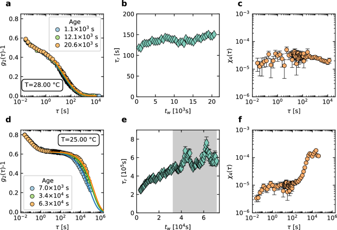
Data obtained with PCI90, q = 22.2 μm−1. a Intensity correlation functions (symbols), averaged over time windows of 500 s, for various sample ages tw. Lines are fits with Eq. (10). b Relaxation time vs tw, showing only marginal aging. c Dynamical susceptibility quantify temporal heterogeneity. d Same as a, but for T = 25.00 °C. e Relaxation time vs tw, note the strong fluctuations for tw ≥ 3.2 × 10⁴ s (gray shaded region). f Dynamical susceptibility during the age interval marked in gray in (e), hinting at the characteristic peak observed for glassy, heterogeneous dynamics. Panels b, c, e, f error-bars (1 standard deviation are calculated using the covariance matrix of the respective fit and are shown only when larger than the symbol size.
The scenario is very different for the sample cooled at lower T = 25 °C, corresponding to a larger φ. Figure 9d shows representative autocorrelation functions for various tw. The separation between the fast decay and the slow structural relaxation is more marked than for the sample at T = 28.00 ∘C, and aging is more pronounced, as highlighted in Fig. 9e. Two aging regimes may be distinguished. Initially (tw ≤ 3 × 10⁴ s), τr increases by more than a factor of two. After this strong aging, the system enters a dynamical state characterized by an overall mild aging, but with large fluctuations of the relaxation time (gray shaded region in Fig. 9e). These differences are accompanied by an evolution of the stretching exponent, which increases from β = 0.541 ± 0.003 for tw ≤ 3600 s to β = 0.63 ± 0.01 during the last hour of the experiment. Dynamic heterogeneity in the second regime is well captured by χ4, Fig. 9f. The dynamic susceptibility shows a very pronounced increase for long delays, hinting at a peak for τ ≈ 2 × 10⁴ s. For glassy systems, χ4 typically exhibits a peak on a timescale roughly corresponding to the system average relaxation time61. Here, unfortunately, we do not have access to these long timescales, since the measurement lasted less than a full relaxation of g2 − 1 (see Fig. 9d). However, the strong increase of χ4 up to values about one decade larger than for the supercooled sample at T = 28 °C, the aging behavior, and the marked separation of the cage dynamics and structural relaxation time all confirm that the sample at T = 25 °C is in a glassy, out-of-equilibrium state.
Dynamics driven by NIR laser heating
We leverage the thermo-sensitivity of pNIPAM microgels coupled to the NIR laser of COLIS to demonstrate thermally-driven dynamics in a colloidal glass. The same pNIPAM suspension as in Section “Spontaneous dynamics: aging and temporal heterogeneity” is brought to a glassy state by cooling the sample from T = 30.00 °C to T = 27.00 °C at a cooling rate of (1,{{rm{K}},{rm{min}}}^{-1}). In the glassy state, the NIR laser is used to impose a cyclic perturbation, as shown in Fig. 10a. In the ON state, the NIR laser power is 300 mW; the duty cycles is 12.5%, to reduce the overall heat injected in the sample while allowing for a significant T increase during the ON state. We probe the effect of the local heating due to the NIR laser on the glassy dynamics by acquiring speckle images with the PCI90 camera (q = 22.2 μm−1), using a stroboscopic scheme, in the same spirit as in the so-called echo protocol for cyclically sheared samples63,64: two images are collected for each cycle, respectively at the end of the ON status and in the middle of the OFF one, see Fig. 10a.
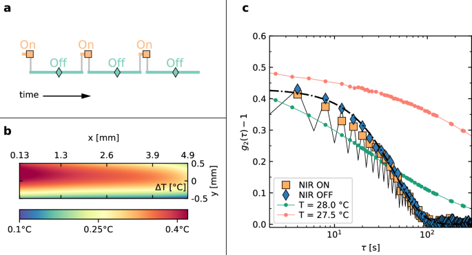
a Temporal scheme of the NIR laser ON–OFF cycles. The duration of the ON and OFF states is 0.5 s and 3.5 s, respectively. The symbols indicate the time at which PCI90 images are acquired. b Local temperature increase during the ON status. c Intensity correlation function for a pNIPAM glass prepared at T = 27 °C, measured at q = 22.2 μm−1). Symbols: g2 − 1 obtained by correlating images taken while the NIR has the same status (ON or OFF, as shown by the legend). The two correlation functions are very similar, only the result of a fit with Eq. (10) of the OFF status is shown for clarity (dot-dashed line). Black solid line: total correlation function calculated starting from an OFF configuration. Green and orange line and small symbols: correlation functions measured with no NIR laser perturbation, for T = 28 °C and T = 27.5 °C, respectively.
Figure 10b shows ΔT(r), the local temperature increase during the ON status with respect to the OFF status. The map has been calculated by averaging 10 speckle images for each status, following the procedure introduced in Section “Space-resolved measures of NIR-induced heating”. The average ΔT is ~0.4 °C, starting from T = 27.4 °C in the OFF state. Interestingly, the temperature map is qualitatively different from that for continuous NIR heating, shown in Fig. 6b. This difference stems from the heat diffusion timescale, whose order of magnitude is d2/α ~10 s, with d ~1 mm the typical length-scale and α ≃0.15 mm2 s−1 the thermal diffusivity of water. Since the duration of the ON status is much shorter than the time needed for heat to be dissipated, we observe here an almost ‘instantaneous’ temperature profile which is marginally influenced by the boundary conditions imposed by the thermalized cell walls. In Fig. 10b, the NIR laser enters the sample from the left and is attenuated during propagation, due to absorption. This is clearly reflected in the temperature map, with a hotter region where the laser enters and a cooler one on the exit side.
The stroboscopic acquisition scheme adopted here reveals the effects of the NIR cycles on the sample dynamics. In Fig. 10c, we show g2 − 1 functions computed correlating images taken during only the ON or OFF status (yellow squares and blue diamonds, respectively). The two correlation functions are very similar; a fit with Eq. (10) yields τr = 76 ± 1 s and β = 1.33 ± 0.04 for the ON status, and τr = 73 ± 1 s and β = 1.44 ± 0.04 for the OFF status (dot-dashed line in Fig. 10c). By contrast, if the correlation function is calculated for all the acquired images (both ON and OFF, black solid line), the curve shows an oscillating pattern, with lower values when correlating configurations taken at different T. This behavior is reminiscent of that of soft solids under oscillating shear65,66. For a small number of imposed cycles (t < 10 s), the cycles of swelling and de-swelling of the pNIPAM microgels play a role similar to that of small-amplitude periodic shear, with the sample almost returning to its previous microscopic state after each cycle. For larger number of applied cycles, microscopic rearrangements add up, eventually leading to the full decay of g2 − 1. The analogy with shear-induced plasticity is also reinforced by the shape of the stroboscopic correlation functions. Here, we find β > 1 for a modest perturbation (about 20% decorrelation between successive ON–OFF statuses), similarly to the low-shear regime in ref. 65.
There are, however, obvious differences in the kind of perturbation imposed to the sample: oscillations of the local volume fraction in COLIS, vs a global shear in mechanical tests. In particular, one may wonder if here the loss of correlation is due to spontaneous relaxations occurring in the sample when its effective volume fraction decreases, due to the NIR-induced heating. To address this question, we compare the dynamics during the NIR cycles to the spontaneous dynamics measured with no NIR beam at two relevant temperatures: T = 27.5 °C, close to the average sample T in the OFF status, and, as a limiting case, T = 28.0 °C, the maximum local T observed in the ON status. Figure 10c shows that the g2 − 1 functions at rest have both a longer decay time and a more stretched shape as compared to those measured while cycling the NIR laser, thus confirming that the latter induces additional plastic rearrangements, distinct from the spontaneous dynamics.
Discussion
The ground tests performed on COLIS have validated the numerous functionalities of the setup. Dynamic light scattering measurements, both polarized and depolarized, yielded translational and rotational diffusion coefficients of Brownian particles fully consistent with expectations from the particle specifications and from independent measurements on conventional laboratory setups. Furthermore, PCI and DLS data have been shown to be fully consistent with each other. A peculiar feature observed for PCI170 and DLS170 is the low-angle scattering contribution due to particles illuminated by a small fraction of the incident beam that is back-reflected at the SALS exit windows. The magnitude of this contribution depends on the refractive index of the solvent, which determines the reflection coefficient at the sample-window interface, and the relative magnitude of the forward scattered intensity compared to back-scattering. This effect can be mitigated in laboratory setups, e.g., by immersing the sample cell in a larger index-matching vat. Here, it cannot be avoided, due to the design constraints inherent to a flight apparatus, as well as the need to include an optical window for collecting SALS data.
We demonstrated both static and dynamic SALS on diluted colloidal particles. SALS data are notoriously affected by stray light: when subtracting an optical background measured with the cell filled by the solvent, the static I(q) was successfully measured down to scattering vectors as small as 0.4 μm−1, while I(q) was overestimated by at most a factor of 2 at smaller q, due to imperfect background correction. Dynamic SALS was successfully demonstrated down to ~0.5 μm−1, data at lower q being affected by stray light and residual sedimentation and convection. This test was particularly stringent, since no optical background correction was implemented, and the sample was particularly sensitive to stray light, since the particles used in the test gave a SALS signal smaller than that expected for typical flight samples, such as colloidal gels.
The experiments on protein crystallization demonstrated that cell D of COLIS allows for very fast and reproducible T quenches with minimal T undershoot. DLS performed in short runs, coupled to absorbance measurements, was successfully used to follow in detail the formation of nucleation precursors in lysozyme solutions and to measure crystallization induction times, with results fully consistent with previous works. In particular, DLS was able to resolve both larger clusters and individual small protein molecules, with Rh = 2.4 nm.
The use of an auxiliary NIR laser beam to locally heat the scattering volume, for water-based samples, and space-resolved light scattering (PCI) are among the most innovative features of COLIS. We leveraged the space resolution afforded by PCI and the change of scattering intensity with temperature of a concentrated suspension of pNIPAM to establish maps of the local heating induced by the NIR beam. This approach allowed us to measure the transient response to a time-varying NIR illumination, as well the T map in the steady state. Note that the latter would not have been accessible using the approach of previous works, based on the T dependent emission of fluorophores dissolved in water67,68, because of convection motion that would have continuously stirred the solvent. The dense pNIPAM suspensions used here, by contrast, should be regarded as an effective porous medium with nanometer-sized pores, which strongly hamper water advection. The NIR experiments have furthermore showed that the dynamics of glassy samples may be significantly sped up with swelling-deswelling cyclces, paving the way for investigating the yielding transition in an original driving mode, complementary to the extensively studied mechanical shear69. In the absence of NIR driving, we were able to measure glassy relaxations and dynamic heterogeneity on time scales up to several 105 s, demonstrating the excellent thermal and mechanical stability of COLIS.
The numerous measurement lines, the use of detectors with complementary features, e.g., the relatively slow, multi-element CMOS cameras and the fast, single-element APDs, the blending of scattering and imaging capabilities, and the advanced thermal control of the sample environment, including with the NIR laser, make COLIS a unique apparatus for investigating the structure and dynamics of soft matter in microgravity. Although COLIS has been primarily designed for measuring weakly scattering systems in Fourier space, its flexible design allows for extensions to other samples and experimental configurations. Examples that may be of interest to the community include using the SALS camera and the PCI170 and DLS170 lines for diffusing wave spectroscopy70 measurements on strongly multiple scattering samples, in the transmission and backscattering geometry, respectively, or using COLIS as a low-magnification multi-view imaging system, through the PCI lines.
Methods
Materials
Brownian particles for the DLS measurements of Section “Polarized DLS” were nearly monodisperse polystyrene (PS) particles of 2R = 277 nm (Invitrogen, standard deviation of the size distribution: 6 nm as reported by the manufacturer) suspended in a 80/20 w/w (weight by weight) mixture of glycerol and water at temperature T = 25 °C, with refractive index n = 1.444 and nominal viscosity of 0.045 ± 0.005 Pa s, yielding a nominal diffusion coefficient of 0.035 ± 0.004 μm2 s−1. The particle volume fraction φ was lower than 10−4.
For DDLS, Section “Depolarized DLS”, we used a φ = 10−2 aqueous suspension of Hyflon MFA, a copolymer of tetrafluoroethylene (TFE) and perfluoromethylvinylether (PF-MVE), produced by Solvay-Solexis S.p.A., Bollate, Italy. The colloids are spherical particles with an average radius of R = 90 ± 2 nm and a polydispersity of 4%, as determined by DLS on a laboratory-based conventional setup. They have a low refractive index (np = 1.352), allowing for index matching for single scattering investigations at arbitrary φ. Furthermore, MFA particles can be roughly pictured as a collection of polymer crystallites, embedded into an amorphous matrix. As a consequence, the particles are optically anisotropic, thus allowing for DDLS measurements. The same particles, but at higher φ = 0.2, where used to form the colloidal gels studied in Sec. Gelation and collapse of a physical gel. To screen electrostatic repulsions, approximately 100 mM of NaCl were added to the suspension. Triton X100, a non-ionic surfactant, was used at a volume fraction ϕT = 0.05, both as a steric stabilizer and as a depletant agent71, to induce attractive interactions53. Finally, about 8% w/w of urea was added to the suspension to fully match the particle refractive index at room temperature. Note that in this system the strength of the depletion interactions may be changed by varying temperature, thus providing a convenient way to induce gelation or redisperse the suspension54,56,71.
For testing SALS, Section “Small-angle static and dynamic light scattering”, we used a suspension of silica (SiO2) particles for static light scattering and a suspension of PS particles for dynamic light scattering. The SiO2 particles (microParticles Gmbh) had 2R = 2.01 ± 0.03 μm and refractive index np = 1.42; they were suspended in MilliQ water, at φ = 2 × 10⁻⁵. The PS particles (Invitrogen CML Latex) had a radius of 230 ± 9 nm and where suspended at a volume fraction of 8.4 × 10⁻⁵ in a 78.2/21.8 w/w mixture of water and glycerol at a temperature T = 25 °C, with refractive index n ≈1.36 and nominal viscosity of 1.61 ± 0.05 mPa s, yielding a nominal diffusion coefficient of 0.59 ± 0.02 μm2 s−1. The particles and solvent density were nearly matched, ρPS ≈ ρsolvent ≈ 1.05 g cm−3, to minimize sedimentation effects.
The colloidal glasses used in Sections “Space-resolved measures of NIR-induced heating” and “Spontaneous and driven dynamics of a soft colloidal glass” are the same as those to be used for the experiments onboard the ISS. They are water-based, concentrated suspensions of poly-N-isopropylacrylamide (pNIPAM) microgel particles with ultralow crosslinking density48,72, which reduces their scattering cross section thereby making them suitable for single scattering experiments. In the range 18–30 °C, the particle radius R decreases with temperature, due to the change of affinity of the polymer chains with the solvent73. For our microgels, R = 130 nm at T = 25 °C, as measured by DLS. The mass concentration was 34 g/L, corresponding to an effective volume fraction of 1.30 at T = 25 °C [see e.g.,74 for how the effective volume fraction is calculated from the known mass fraction; note that effective volume fractions larger than one are possible for deformable, interpenetrable particles such as our microgels.]
For the protein experiments of Section “Using COLIS to study protein nucleation”, lysozyme stock solutions were prepared by dissolving 7 mg/ml lyophilized lysozyme (PanReac Applichem 232-620-4) in a sodium acetate buffer (50 mM, pH 4.5). The pH was adjusted with HCl to give the desired pH 4.50. The solutions were filtered two times (0.2 μm filters) to remove all undissolved protein particles and dialyzed two times against the buffer to remove the excess salt of the lyophilized lysozyme. For each dialysis step, 100 ml of solution was dialyzed in 2 l of buffer for 24 h. The membranes used for the dialysis were Spectra/Por 3 with a 3.5 kD cut-off. After dialysis, the concentration of lysozyme was determined by spectrophotometry. For a concentration measurement, the stock solution is dissolved (dilution factor 200–500) and absorbance was measured at 280 nm using a CARY 100 Bio spectrophotometer and an absorption coefficient of e = 2.64 ml/mg was used to determine the concentration. The precipitant stock solutions of NaCl solutions were prepared separately by dissolving the appropriate amount of NaCl in the same buffer and Sodium Azide was added in order to neutralize any biological contamination. After complete dissolution of NaCl and NaN3, all solutions are filtered to 0.2 μm to remove any undissolved material. The lysozyme and NaCl stock solution are finally mixed to obtain the final concentrations. Typical concentrations of lysozyme, NaCl and NaN3 in the mixed samples are 7 mg/ml, 65–70 mg/ml, and 0.5 mg/ml, respectively.
Responses