An approach to assessing tsunami risk to the global port network under rising sea levels

Seaports are vulnerable to extreme sea level events, such as coastal floods, storm waves and tsunamis^1,2,3. Unlike coastal floods and storms which are mostly localised events, tsunami waves have a proven reach where a singular event can damage several ports at once, even those of thousands of kilometres away⁴. The 2004 Indian Ocean tsunami, for instance, damaged port facilities across the Indian Ocean including those in Indonesia, Thailand and Sri Lanka⁵. On the same note, the 2011 Great East Japan (Tohoku) earthquake-tsunami resulted in damage to 14 ports along the Tohoku Region in Japan, and a number of small craft harbours along the west coast of the United States^4,5.

The impact of a tsunami on ports has considerable economic consequences beyond physical damage. Damage to port facilities and vessels by the 2011 Tohoku tsunami cost up to US$12 billion⁶, but losses in seaborne trade due to port disruption was estimated at US$3.4 billion a day in the months following the tsunami⁷, highlighting the large disparity between the primary and secondary effects of a port damage. However, academic literature on the impact of port disruptions due to tsunami events is lacking. To the best of our knowledge, Rose et al.⁸ represents the only study that attempts to evaluate the impacts of a port shutdown due to tsunami. Rose et al. ⁸ provided a comprehensive evaluation of the potential economic impacts that would arise as a result of a port shutdown in California due to a far-field tsunami. The study assumes that a far-field tsunami would likely result in a two-day port shutdown but it does not establish a relationship between tsunami hazard intensity and the scale of port disruption. Past studies have demonstrated that tsunami hazard intensities e.g. inundation height and wave velocity can influence the extent of damage to port structures and accordingly, the duration of port recovery^5,9,10.

A number of studies have assessed the economic consequences of exogeneous shocks on ports, including those of natural hazards such as storms and coastal floods^11,12. Most studies are port-centric, where the focus is on the economic impacts caused by a port shutdown at individual ports. Common assessment indices used include (i) direct losses in cargo throughput¹¹ or (ii) indirect sector-based economic losses through the use of multi-regional input-output (MRIO) models^8,13,14. The latter is more widely used in literature and considers the macroeconomic impacts caused by a port disruption—localised to the regional or national economies of the affected port.

Any port inoperability does not only affect trade flows in and out of the affected port, it also disrupts shipping routes connected to it which then propagates throughout the rest of the global port network. The past decade has seen the emergence of network-centric approaches to assessing the vulnerabilities of port networks to port disruptions^15,16,17. Network-centric approaches treat maritime traffic as a network graph with ports as its nodes and shipping routes as its edges. The impacts of a disruption are quantified by changes to the topological properties of the network. Few studies have attempted to integrate both port- and network-centric measures in their risk assessments of port disruptions. However, a comprehensive picture of the potential risks across the domains – from individual ports to the entire port network, is necessary for the different stakeholders i.e. port authorities, port operators, shipping and logistics companies to work together to minimise the impacts of port disruptions.

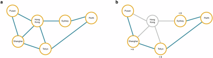
Here, we present a framework to assessing tsunami risk to commercial seaports and the global port network. The global port network model in this study is represented by the global liner shipping network (GLSN) since liner shipping forms the backbone of international trade. We set the stage to this study and future studies by establishing the criteria for port disruption in a tsunami–an exercise which has not been undertaken in the literature. Observations from the 2011 Tohoku tsunami indicate that a tsunami elevation of 3.3 m above mean sea level is sufficient to damage port structures, leading to disruption¹⁸ (Fig. 1a, b). Numerical simulations of tsunami scenarios are performed to derive tsunami heights and identify the ports-at-risk. Port-specific risk is quantified by the direct economic losses that an affected port is likely to sustain due to loss in trade during the period of port disruption. Using observations from past, modern tsunami events, we draw the relationship between maximum tsunami height and period of port disruption. Risk to the port network is evaluated by examining the changes in the topological properties of the GLSN before and after a disruption, through the use of centrality measures.

a Locations of tsunami heights recorded at ports along the Pacific coast of eastern Japan during the 2011 Great East Japan tsunami. b Tsunami heights measured against mean sea level, adapted from Ministry of Land, Infrastructure, Transportation and Tourism (www.mlit.go.jp/common/000142288.pdf). Minimum height observed at damaged ports was 3.3 m (Onahama Port) and this is set as the threshold height required to disrupt a port’s functions. c Maximum tsunami height is measured against present-day mean sea level (MSL). Assuming the design heights of port structures remain unchanged in future sea level scenarios (to 2100), maximum tsunami heights (Zmax_present) under future scenarios are also referenced to present-day sea levels.

Full size image

To illustrate our objectives, we apply our risk framework to a potential tsunami scenario in the South China Sea region. The South China Sea region is home to some of the world’s busiest ports. Approximately 21 of which are ranked amongst the world’s 50 busiest ports in 2021¹⁹. The tsunami threat within the South China Sea region is generally underestimated, due to the lack of historical records and poorly constrained geological records in the region^20,21,22. The Manila subduction zone has been postulated as a potential source of tsunami in the South China Sea region^23,24. Previous studies^25,26 have demonstrated that the Manila megathrust is capable of producing basin-wide tsunami waves. With many major ports concentrated in the region and most of them located in low-lying coastal areas, a tsunami event from the Manila trench could result in detrimental economic consequences beyond the affected port(s).

Capital planning cycles at ports typically span 5 to 10 years²⁷, which implies that disaster mitigation plans are inadequate in facilitating high-impact, low-frequency events such as tsunamis which recurrence intervals typically exceed 100 years. Moreover, tsunami threats to port assets are expected to be exacerbated by rising sea levels. Most present-day port structures are unlikely to have been designed with climate-related sea level rise in mind, as port structures are typically designed for 30–50-year life cycles but often remain in service for up to 100 years^27,28.

Coverage of sea level rise effects on tsunami hazards in the existing literature is relatively limited^29,30,31. The few studies which consider the effects of sea level rise in future tsunami events apply a spatially uniform height of sea level rise, often a global mean sea level rise, in their tsunami numerical simulations^32,33,34. This was by and large because local sea level rise information has been, up to now, limited for most regions e.g. Asia and Africa. However, it is prudent to note that the rate and magnitude of sea level rise is expected to differ from region to region due to differences in thermal expansion, changes in vertical land motion, e.g. subsidence, tectonic activity and glacio-isostatic adjustment etc.^35,36, and a one-size-fits-all global estimate may lead to a severe under- or overestimation of future tsunami hazards. With the advent of the Intergovernmental Panel on Climate Change (IPCC) Sixth Assessment Report (AR6)³⁷, local and regional sea level rise projections have become more accessible, and this study presents the first attempt to integrate spatially varied local sea level projections in potential tsunami scenarios.

Overview of network topology and centrality measures

In a global shipping network topology, ports are represented as nodes and the routes that ships travel between two ports are represented as edges. It is important to note that liner (container) ships travel along service routes between a port of origin and a port of destination, and they consecutively call at intermediate ports between these two points. The topology of a global shipping network can be represented in what are known as L-space and P-space graphs. In an L-space, an edge exists only when it is between two consecutive port calls³⁸. Whereas in a P-space graph, an edge exists as long as the pair of ports lie on the same service route–regardless of the order of port calls.

Centrality indices of a port are conventionally used to measure the connectivity of a port to other ports within a network³⁹. Amongst centrality indices, degree centrality is amongst the most common. Degree centrality, as introduced in Freeman⁴⁰, measures how popular and well-connected a node is within the network, and can be calculated by

, where ({k}_{i}) represents the number of edges connected to node (i) and (N) represents the total number of nodes. Betweenness centrality (BC) measures the importance of a node in the overall network by defining the degree in which a node lies in the shortest path between a pair of other nodes⁴⁰. In the case of a global liner service network, a port with a higher BC score would have a greater importance in the network as it represents the number of times that port serves as a point of accessibility between other pairs of ports. Using Freeman’s⁴⁰ definition, an unweighted BC score of a single node can be calculated as follows:

, where N is the number of shortest paths passing between start (s) and end (t) nodes, and ({n}_{i}) is the intermediatory node that lies on the shortest path between (s) and (t). ({{n}}_{{i}_{s,t}}) is 1 when node ({n}_{i}) lies on the shortest path between (s) and (t), and 0 when it does not. A conceptual model of a shipping network is shown in Fig. 2 to illustrate the concepts of the two centrality measures.

Changes in network (a) before a disruption, and (b) after a disruption to illustrate the concepts of degree and betweenness centralities. Nodes (seaports) are represented by yellow circles and the blue lines connecting between two nodes represent edges (service routes between two ports). In (a), Hong Kong represents a port with the highest degree of centrality as it connects to the greatest number of nodes, and it also possesses a high betweenness centrality as it lies in the shortest paths to most other nodes. In (b), an event resulted in the loss of the functions at Hong Kong port. Shanghai and Tokyo serve as alternative ports to travel between Pusan and Perth, and hence, the ratio of change in betweenness centrality is greater than 0. As the service is rerouted, Sydney no longer serves as a port between Pusan and Perth, resulting in a less than 0 ratio.

Full size image

Busiest ports in the South China Sea region

A GLSN was constructed for this study using the data provided by Xu et al. ⁴¹, who collected liner service routes in 2015 from 489 shipping liner companies. After data cleaning on the original dataset, a total of 966 nodes (ports) and 16,533 edges (routes) have been identified and used for our analysis (Fig. 3a). Due to the simplicity of the data available, this study assumes an unweighted and undirected network in a L-space graph (see Methods).

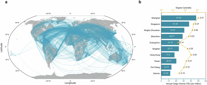
a Liner service routes from 489 shipping liner companies in 2015. Each point (node) represents a port. Each line (edge) represents the route (voyage leg) between any two ports. There are a total of 966 nodes and 16,533 edges. The dataset is adapted from Xu et al.⁴¹. b Ten busiest ports in the South China Sea region by degree centrality (yellow dots) and annual cargo volume (blue bars).

Full size image

We selected the 10 busiest ports within the region to demonstrate the application and interpretation of our approaches for the remainder of the study. We relied on the degree centrality of each port as well as their annual cargo throughput to identify the 10 most important ports within the South China Sea region (Fig. 3b). The 2020 annual cargo throughput was obtained from the World Shipping Council¹⁹ and quantified in twenty-foot equivalent unit (TEU) cargo capacity for container ships. It could be observed that annual cargo throughput does not directly reflect the relative rankings of degree centrality. For instance, the annual cargo throughput volume of Guangzhou is greater than that of Qingdao, but the opposite is true for the degree centrality scores. This is one of the limitations of using an unweighted graph, where the true volume of trade flow impacted during a port disruption cannot be properly reflected. This is also one of the limitations of the study, it nevertheless does not hinder us from illustrating our objectives.

Damaged ports at present-day sea levels

Eight potential sources of earthquakes originating from three different segments of the Manila Trench were proposed by Qiu et al.²⁶ (in Supplementary Fig. 1a, b). The earthquake scenarios, which range from M_w 8.9–9.1, are capable of generating basin-wide waves across the South China Sea. Tsunami waves generated from zone 1 (the southernmost segment-14–16°N) of the trench produce the greatest tsunami heights, especially in the near-field and intermediate near-field regions (Supplementary Fig. 2a, b). Maximum tsunami heights exceed 9 m in western Luzon, Palawan (the Philippines) and the eastern Vietnamese coasts. Zone 2 (16–19°N) does not generate tsunami waves as high as those of zone 1, but the waves are far-reaching–extending to far-field areas further up north such as the southeastern coast of China and the south of Taiwan. Tsunami waves from zone 3 (the northernmost segment 19–22°N) are generally directed towards the northern part of the South China Sea region, affecting the coasts of southeast China and south Taiwan. Unsurprisingly, the spatial distribution of maximum tsunami heights is similarly reflected in the spatial distribution of ports that are likely to be damaged.

Given our established damage criteria of 3.3 m in tsunami heights, we identified ports that are likely to be damaged and hence, disrupted in the eight earthquake scenarios. Tsunamis originating from zones 1 and 2 will damage a greater number of ports (n = 7–11) compared to those from zone 3 (n = 3–6) (Supplementary Fig. 2a, b). Ports in the southeastern coasts of China i.e. Hong Kong and Zhuhai, as well as Kaohsiung port (south Taiwan) are amongst the most vulnerable in a Manila Trench tsunami. Hong Kong and Zhuhai are consistently damaged in all scenarios, whereas Kaohsiung port is damaged in tsunamis originating from zones 2 and 3. With Kaohsiung and Hong Kong ports being amongst the world’s 50 busiest ports, a Manila Trench tsunami can have dire consequences for maritime trade and the local economy in these ports. Despite zone 1 generating greater tsunami heights, scenario Z2B (zone 2) represents the worst-case scenario, where up to 11 ports are being damaged (Fig. 4). Z2B forms the basis of our analysis for the remainder of the study as it provides the upper bound of the expected risk in a Manila Trench tsunami.

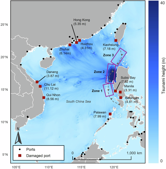
Scenario Z2B represents the scenario with the greatest number of damaged ports (n = 11). Black dots represent seaports and red squares represent damaged ports. Boxes in purple show the general rupture zones of the slip models proposed in ref. ²⁶.

Full size image

To assess the potential direct economic losses that would be caused by a disruption at the port, we quantified the volume of cargo throughput that will be lost in the period of disruption. Fig. 5 shows the relationship between tsunami heights and days of disrupted port activity from past tsunami events, i.e. the 2010 Chile, 2011 Great East Japan, 2015 Illapel, 2018 Palu and 2018 Krakatoa tsunamis. A total of 23 damaged ports were identified from these events. Each curve, accompanied by its bootstrap estimates, represents different operation status, i.e. shutdown, partial operation and total affected days. A port is considered to have shut down when no port calls could be made, and operating partially when berthing is at limited capacity. The total affected days are a sum of both. The correlation coefficients of the linear regression models differ vastly between the curves. The correlation is highest (~0.41) for shutdown, and lowest (~0.08) for partial operation. This is unsurprising, considering that the partial operation status is assumed to be a mutually exclusive event when in fact, a port may be shut down for a period before operating at reduced capacity. The correlation for the total affected days is ~0.19 which is higher than that of the partial operation status, but nevertheless a poorer correlation. This highlights the fact that the recovery process of a port’s functions may not be linear and could be attributed to a myriad of reasons including recovery priorities, the types of dependencies the port components have and the redundancies available.

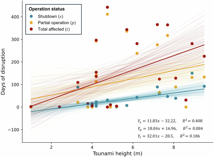
Port is considered (i) shutdown (blue) when no port calls could be made and (ii) operating partially (yellow) when berth activity is at limited capacity. The total affected days (red) is the sum of shutdown and partially operating days. Curves in bold represent the mean linear regression of each operation status and faint lines represent their bootstrap estimates.

Full size image

A Manila Trench tsunami could result in port closure (shutdown) of up to 200 days (Supplementary Table 1), which supersedes those of previous tsunami events (Supplementary Table 2). The 2011 Tohoku tsunami and the 2015 Illapel tsunami resulted in the closure of a maximum of 150 days (Soma Port) and 31 days (Coquimbo Port) respectively. While Z2B represents the worst-case scenario in terms of number of damaged ports, the maximum period of port closure is <100 days. Tsunamis originating from zone 1 result in the longest period of closure. In scenarios Z1A and Z1B, Subic Bay port is expected to remain closed for >200 days and Palawan port for >80 days. In all other scenarios, the ports of Chu Lai (>90 days) and Kaohsiung (>50 days) have emerged as the most affected by port closure. It should be noted that beyond a threshold tsunami height, damage may be so extensive that a reconstruction of port facilities may be required and therefore, the number of disruption days remains the same regardless of tsunami height. However, given the limited observations from past tsunami events, this study has yet to establish the threshold height.

The volume of trade lost due to port closure is calculated as a product of the daily average of the annual cargo volume and the number of port closure days. Supplementary Table 1 shows the estimated trade loss in cargo volume for damaged ports in each scenario. Note that the annual volume of cargo throughput is not publicly available for the ports of Chu Lai and Kota Kinabalu. The greatest losses in cargo volume are consistently observed in the ports of Kaohsiung, Manila and Hong Kong in most baseline scenarios. The volume of trade lost does not necessarily equate to the height of the tsunami experienced by the port, nor does it equate to the number of disruption days. For instance, in scenario Z2B, Qui Nhon port experiences one of the highest tsunami heights (~8.5 m) and an estimated 69 days of shutdown (Table 1a). However, the expected losses for Qui Nhon (>6000 TEU) are almost 1/200 times that of Hong Kong port which has an estimated tsunami height of ~5.3 m and closure of 31 days. In essence, the exposure of a port i.e. its assets, trade activity, trade flow and criticality in the local and regional economy, could have a greater influence on the total risk than the tsunami hazard itself.

In this study, calculations of direct losses are based solely on port closure. Losses during the period of partial operation are not included in the estimations because (i) we have no further information on the degree of reduced capacity at each port and (ii) the recovery process differs from port to port and is highly dependent on the priorities and redundancies available. Therefore, the volume of trade lost calculated here is a conservative estimate and actual losses are likely to be much greater.

Beyond the damaged ports—impacts on the port network

A port disruption can have cascading effects on the rest of the port network. Port inoperability would disrupt port calls and hence, the service routes with scheduled calls at the affected port. We assessed the overall reduction in edges in the port network through the removal of damaged nodes from the GLSN (Fig. 6). Z2B has the greatest impact on the overall port network, with 15,193 edges remaining–a contraction of 620 (or −3.7%) from the original numbers. This is unsurprising, given that Z2B also represents the scenario with the most damaged ports. This is, however, not always the case for other scenarios. Z1B presents the second highest number of damaged nodes (n = 8) with 16,132 edges remaining, but tsunamis originating from Z2A (n = 7) and Z3B Mega (n = 4) have a greater impact on the overall network with 16,039 and 16,072 edges left respectively. It is important to note that each of these edges merely represents the voyage leg between a pair of ports in this study (see Methods). In reality, however, the same leg serves multiple services and the volume of cargo flow differs from leg to leg. A weighted graph of the GLSN considering these factors would provide a more accurate picture of the potential impacts of a tsunami on the overall network, but it is beyond the scope of this study and will be investigated in future work.

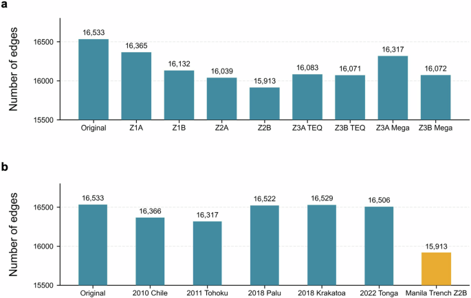
Original refers to the total number of edges in the global liner shipping network dataset. Damaged nodes are removed from the dataset and remaining edges are tabulated. a Proposed earthquake rupture scenarios from the Manila Trench at present-day sea levels. Z2B represents the worst-case scenario as the tsunami likely results in the greatest changes in the overall port network. b Historical tsunami events. A Manila Trench earthquake (>Mw 8.8) could potentially disrupt more shipping routes as compared to previous tsunami events.

Full size image

Compared to past, recent tsunamis, a tsunami from the Manila Trench potentially has a greater impact on the overall port network. For past tsunami events, damaged nodes were similarly removed from the GLSN and the remaining number of edges was measured (Fig. 6b). Using the same baseline dataset allows for a fairer comparison. In terms of earthquake sizes, the 2010 Chile (M_w 8.8) and the 2011 Tohoku (M_w 9.1) events are comparable to the Manila Trench scenarios (M_w 8.8–9.1). We compared past tsunami events with scenario Z2B (M_w 9.1)—the worst-case scenario and found that the number of edges impacted in Z2B is much higher than those in past tsunami events (Fig. 6b). The number of edges lost in the 2010 Chile and 2011 Tohoku tsunamis is comparable only to Z1A and Z3A Mega scenarios respectively, both of which represent the scenarios with the least impacted edges. The uneven impacts on the port network could be due to the criticality of the ports impacted. Because the Manila Trench is situated in the South China Sea region which is home to some of the world’s busiest ports, the exposure is much greater than those of previous tsunami events. For instance, in the 2011 Tohoku tsunami, only a handful of the damaged ports including Kashima, Shiogama and Muroran were serving shipping liners from international ports. Therefore, the number of impacted edges is expected to be much lower than those of the Manila Trench. In addition, because the South China Sea is a semi-enclosed basin of about 1/20th of the size of the Indian Ocean²⁶, tsunami wave energy undergoes less dissipation before arrival on shore which results in greater tsunami heights. The semi-enclosed nature of the basin also means that basin oscillations are pronounced^42,43, and waves are likely to undergo multiple reflections and incidence. As such, a tsunami within the South China Sea basin could be more damaging to assets along coastlines as compared to tsunamis in open oceans.

The roles and functions of ports other than those damaged can be altered by a tsunami. Vessels that are originally scheduled to call at the damaged port, are rerouted to another port which plays the role of substitution. For instance, vessels that were supposed to call at ports in the Tohoku region during the 2011 Tohoku tsunami, were redirected to ports in the Keihin area and the Hokuriku region in the Sea of Japan⁴⁴. In this study, we assume that the ports of substitution are the ports that lie in the alternative ‘shortest paths’ to the next port of call. A new measure proposed in this study, the BC change ratio, is used to assess ports that serve as substitution and ports that lose their scheduled calls (Fig. 2). The BC index measures the number of times a port lies in the shortest paths between a pair of ports. A reduced BC index indicates that the number of service routes that goes through that port is reduced, and vice versa. A BC change ratio of -1 indicates a damaged port, and a ratio of 0 represents no change in the BC before and after a tsunami. A BC change ratio >0 indicates that the number of scheduled calls at the port has increased, and hence, it serves as a port of substitution. On the other hand, a BC change ratio <0 indicates that the number of scheduled calls at the port has decreased and the vessels have been redirected to other ports. BC change ratio maps of each baseline scenarios are presented in Supplementary Fig. 3a,b.

In scenario Z2B, BC change ratios are generally positive in ports within close proximity of the damage ports (Fig. 7a). For instance, ports in the rest of Taiwan experience increased BC change ratios when the port of Kaohsiung is damaged. BC change ratios are most positively pronounced (>0.5) in the Visayas and Mindanao islands in the Philippines, which could be attributed to the four damaged ports (Subic Bay, Manila, Batangas and Palawan) in the neighbouring Luzon and Palawan islands. Similar patterns can be observed in other scenarios (Supplementary Fig. 3a, b). In zone 3 scenarios, when ports in Luzon island are not damaged, the number of neighbouring ports that exhibit positive BC change ratio is reduced—none of which has ratio >0.5. It is therefore expected that the ports of substitution are usually located in geographic proximity to the damaged ports.

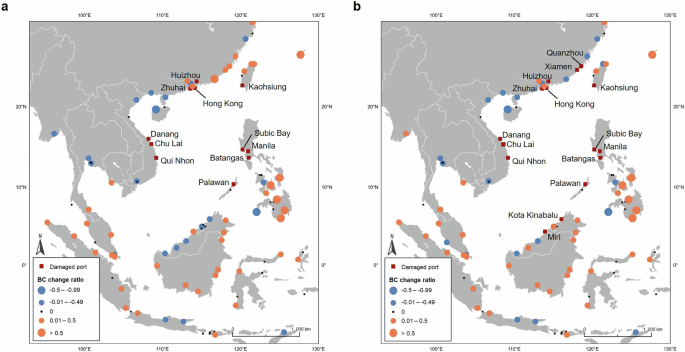
Tsunamis originating from (a) earthquake scenario Z2B under present-day sea levels and (b) earthquake scenario Z2B under SSP 5–8.5 (LC) in 2100. A damaged port (red squares) would have a BC change ratio of -1, as it completely loses its function. A BC change ratio of 0 represents no change in betweenness centrality. A BC change ratio of greater than 0 (orange dots) indicates that the number of times the studied port lies on the ‘shortest paths’ between a pair of ports have increased, i.e. it hence serves as an alternative intermediate port. A BC change ratio of less than 0 (blue dots) indicates that the number of times the studied port lies on the “shortest paths” between a pair of ports have decreased, i.e. scheduled vessels no longer call at the studied port and instead, are redirected to other ports.

Full size image

We selected the ten busiest ports in the South China Sea (Fig. 1b) to examine how they will be influenced by a Manila Trench tsunami (Supplementary Fig. 4). The port of Hong Kong has the greatest number of closures across all baseline scenarios (BC change ratio = −1). The other 9 ports have BC change ratio >0 in most scenarios except Z1A, indicating that they are likely to serve as ports of substitution during a Manila Trench tsunami. A closer look indicates that Shenzhen and Guangzhou ports have the greatest positive BC change amongst the ten ports in most scenarios, which highlights their criticality in serving as substitute ports in a Manila Trench tsunami. It is important to note, however, this study presents an idealised scenario where the capacities of the substitute ports to absorb rerouted vessels are assumed to be infinite. In actuality, ports have specific sizes, number of berths, and varying berth sizes and depths. Berths are also allocated months in advance for scheduled vessels. Therefore, rerouted vessels can overwhelm alternative (substitute) ports, leading to bottlenecks or knock-on effects in trade flows.

Changes in port disruption in future sea level scenarios

The service life of port structures is typically 80–100 years^27,45, and therefore, port planning and design are required to plan for potential sea level rise. The risk of tsunami hazards on ports is also expected to be compounded by sea level rise and should also be considered in design and adaptation plans. For each earthquake scenario, we modelled maximum tsunami heights under different sea level rise scenarios presented in the IPCC AR6 report. We considered medium confidence Shared Socio-economic Pathways (SSP) scenarios i.e. SSP 1–1.9, SSP 1–2.6, SSP 2–4.5, SSP 3–7.0 and SSP 5–8.5 and the low confidence scenario SSP 5–8.5 (LC). Including the sea level projections for 2050 and 2100, we performed tsunami numerical simulation for an ensemble of 96 sea level rise scenarios.

Assuming the design height of port structures remains unchanged to 2100, the criteria for damage in future sea level rise scenarios remains the same, i.e. 3.3 m above present-day mean sea level. Modelled tsunami heights in future scenarios are therefore referenced to present-day mean sea level (Fig. 1c). Tsunami heights are generally higher in 2100 scenarios compared to 2050 scenarios (Supplementary Table 3). Take scenario Z2B for instance, tsunami heights in SSP 1–1.9 and SSP 1–2.6 2100 scenarios are higher than those of SSP 5–8.5 (LC) 2050 scenario, though the former two scenarios represent shared socio-economic pathways of lower consequences and the latter represents the worst case scenario. Nevertheless, the differences in tsunami heights between the shared socio-economic pathways are not obvious. The most noticeable difference is between tsunami heights in SSP 5–8.5 (LC) 2100 scenarios and other scenarios. The number of ports that is likely to be damaged in SSP 5–8.5 (LC) 2100 scenarios are also significantly more than other sea level rise scenarios (Table 2). Take scenario Z2B for instance, up to 15 ports are likely to sustain damage (Fig. 7b), a stark contrast to the 11 and 12 ports damaged in the baseline scenario and the medium confidence scenario SSP 5–8.5 in 2100.

A closer examination of scenario Z2B paints a picture of the uneven impacts of sea level rise for port risk. When comparing SSP 5–8.5 (LC) 2100 projections with the baseline scenario, we observe that tsunami heights in the southeastern coasts of China, e.g. Zhuhai and Hong Kong tend to be ≤1 m higher than the baseline scenario, whereas tsunami heights along coasts east of the Manila Trench, e.g. Manila and Palawan are ≥1 m. Such spatial differences could be attributed to the transformation of tsunami wave as it transverses the continental shelf westward of the Manila Trench towards the southeastern Chinese coasts. A preliminary investigation into the tsunami numerical simulation output indicates that tsunami heights are amplified as the wave propagates from deeper waters onto the shallower continental shelf, in line with the findings of Naik and Behara⁴⁶. With sea level rise, the water column above the continental shelf becomes deeper and conversely, deformation of the tsunami wave is reduced and tsunami height becomes less amplified. However, this requires detailed investigation and will be considered in future work.

Despite changes in tsunami heights being uneven spatially across the South China Sea basin, the economic consequences are far greater for ports located in the southeastern coasts of China, as they host some of the busiest ports, e.g. Hong Kong, Xiamen and Zhuhai in the region (Table 1b). Direct economic losses in terms of cargo throughput, in ports along the southeastern coasts of China are likely to exceed those along the coasts east of the Manila Trench, e.g. Manila, Kaohsiung, and Palawan in the worst-case scenario–SSP 5–8.5 (LC) by 2100.

The number of edges disrupted in 2100 sea level rise scenarios are higher than those of the 2050 scenarios—in line with the differences in the tsunami heights (Supplementary Fig. 5). The number of edges lost in 2050 scenarios do not differ much from the baseline scenarios, whereas the difference is more apparent between the baselines and the 2100 scenarios. Interestingly, in a few instances, e.g. Z1A, Z1B, Z2B, the number of edges lost in future scenarios is estimated to be fewer than present-day (baseline scenarios). This could be attributed to the spatially uneven changes in tsunami heights under sea level rise conditions. Ports that sustain damage and lose their functions under present-day conditions, may not be as severely impacted in future scenarios. Some of these ports could likely have critical positions (connected to more edges) within the port network, and therefore, have a greater impact on the network when damaged.

We examined changes in BC for the 10 busiest ports in South China Sea, similarly for sea level rise scenarios. Supplementary Fig. 6 shows the changes in BC change ratio for all SSP scenarios for 2050 and 2100 projections. The port of Hong Kong is expected to lose its functions in all sea level rise scenarios; and Xiamen is likely to lose its functions only in 2100 projections for SSP 2–4.5, 3–7.0, 5–8.5 and 5–8.5 (LC) scenarios. The remaining ports generally have a positive BC change ratio, with Guangzhou and Shenzhen displaying greater positive BC change ratio, which underscores their importance in serving as substitute ports in a future Manila Trench tsunami.

This study presents a first attempt at assessing tsunami risk to the global port network. We provided a risk assessment framework that quantifies risk at port and network scales. For the first time, a criterion to identify ports at risk of damage and disruption by a tsunami is being established. The risk framework was applied to the South China Sea region where tsunami risk from a Manila Trench earthquake was being evaluated. Various potential earthquake sources were considered to provide an upper bound to the expected risk in a Manila Trench tsunami. We also introduced an approach to assessing damage to ports under rising sea levels, and adopted sea level projections of multiple SSP scenarios from the latest IPCC AR6 for our risk assessment. In total, an ensemble of 104 tsunami scenarios were considered in this study.

Earthquake scenario Z2B represents the upper bound of the tsunami risk, where up to 11 ports are likely to be damaged at present-day sea levels and 15 ports under SSP 5–8.5 (LC) sea level rise scenarios. Ports can remain closed up to >200 days in a Manila Trench tsunami, which supersedes those of previous major tsunami events such as the 2011 Tohoku and 2015 Illapel tsunamis. Tsunamis can cause a longer period of port disruption than most meteorological hazards. Hazards such as heatwaves, precipitation and fog cause disruption in order of a few hours⁴⁷, while tropical cyclones can cause disruption in order of 4–22 days⁴⁸. Earthquakes, on the other hand, can cause damage of similar magnitude or greater to port structures. For instance, the 1995 Kobe earthquake caused severe damage to Kobe port and a full recovery of the port took up to 2 years⁴⁹. It is also important to note that the damage associated with tsunamis may not be solely caused by the tsunami alone, but rather a combination of both the preceding earthquake and the subsequent tsunami as evident in the 2011 Tohoku event⁵.

Port-specific risk was quantified in this study by direct losses in cargo throughput. The greatest losses in cargo volume across most baseline scenarios are the ports of Hong Kong, Kaohsiung, and Manila. The volume of trade lost does not necessarily equate to the tsunami height and number of disruption days that a port experiences. Rather, the exposure of the port, i.e. its assets, trade activity and criticality in the local and regional economy, could have a greater influence on the total risk than the tsunami hazard itself. This study only considers direct losses from disruption to trade flows. Future studies can and should extend our proposed framework to estimate indirect, sector-based losses for the regional and national economies through MRIO models. Knowing the port-specific risk can aid port authorities and operators in their development of mitigation plans to reduce damage and period of recovery, as well as adaptation plans to remain competitive after a long period of closure.

We leveraged the topological properties of the GLSN and centrality indices to assess tsunami risk at a network level. Compared to past modern tsunami events of similar magnitudes, a Manila Trench tsunami is likely to impact more shipping routes (−3.7% of the total edges compared to −1.3% during the 2011 Tohoku tsunami). This could be attributed to the criticality of the ports impacted in a Manila Trench event, as the South China Sea region hosts some of the world’s busiest ports including Hong Kong and Kaohsiung. Additionally, because the South China Sea is a semi-enclosed basin, wave energy undergoes less dissipation as compared to open oceans and therefore, tsunami heights can be expected be greater given similar earthquake magnitudes.

A new measure–the BC change ratio was proposed in this study to reflect changes in the functions of ports beyond the affected. Ports in geographic proximity to the damage ports are found to be likely candidates for port substitution in a tsunami event. Using similar approaches, potential substitution ports can be identified in other scenarios and assist logistics and shipping companies in developing business continuity plans.

The impacts of sea level rise on tsunami risk were found to be uneven throughout the South China Sea region. Increase in tsunami heights under the most extreme sea level scenario SSP 5–8.5 (LC) was found to be greater to the east of the Manila Trench–along the west coasts of the Philippines and southern Taiwan. The increase in tsunami heights was relatively lower in the eastern coasts of China and Vietnam. Despite such spatial differences, economic losses for ports in the southeastern coasts of China exceed those of ports in the Philippines and Taiwan, which emphasizes the role of exposure in the overall risk and the greater need for asset protection.

Some caveats should be noted in this study. An unweighted GLSN was used to demonstrate the application of our risk framework, and its topology properties were assumed to be static in this study. However, the global shipping network is intrinsically dynamic and evolves over time. We encourage future research to account for the cumulative weight of services that pass through the nodes to reflect not only the true criticality of the node in the overall network, but also the potential flow of trade that would be disrupted in a tsunami event. The application of the risk framework proposed in this study to the South China Sea region is limited by the availability of data such as the volume of trade flows in the GLSN. However, the framework is transferable to other regions and other tsunami scenarios, and assist port authorities, operators, and shippers in the management of tsunami-related risks and the development of adaptation plans.

Earthquake scenarios from the Manila Trench

The Manila subduction zone is located at the boundary where the Sunda Plate converges with the Philippine Plate. Despite having one of the fastest rates of convergence in the world and hence being seismically active, no earthquakes larger than Mw 7.6 have been recorded since 1560^23,24. The absence of megathrust earthquakes in modern records suggests that the fault is locked and accumulating strain energy which could be released as a giant rupture⁵⁰.

Several studies in the past have proposed fault models for the Manila subduction zone^23,26,51. The Manila subduction zone is capable of producing M_w > 8.0 earthquakes and hence, adequately sized tsunamis in the South China Sea region^52,53. However, Li et al. ²⁹ have demonstrated that at present-day sea levels, earthquakes of magnitudes less than M_w 8.6 are likely to generate relatively small tsunamis with negligible impact on the southeastern Chinese coasts. In this study, we selected the deterministic fault models proposed by Qiu et al. ²⁶ to model potential tsunami waves generated by Manila Trench and its consequent impacts on the South China Sea coastlines. Qiu et al. ²⁶ proposed a series of possible fault rupture models (M_w 8.8–9.1) from the Manila subduction zone based on both the local geological structures, slip deficit rates and characteristics of other subduction zone earthquakes. The subduction zone is divided into three fault segments (Zones 1–3) using the seamount chain as a boundary. Each segment assumes a seismic return period of 1000 years. Earthquake sources were built based on the coupling models established in ref. ²⁴. However, the coupling state of the northern segment (Zone 3) is poorly resolved due to the sparse GPS network²⁴. Additionally, various seismic structure analyses within this segment indicate that the outer wedge of the accretionary prism has developed many high-angle, imbricate and mega-splay faults⁵⁴. High-angle faults have been observed to produce outsize tsunamis, which are generally unexpected due to their relative seismic magnitudes, at global subduction zones⁵⁴. To account for the tsunami potential of the Manila Trench, variable earthquake sources (e.g. tsunamigenic earthquake and megathrust-splay fault) were proposed for the northern segment. Readers are recommended to refer to refs. ^24,26 to better understand how the fault models are being developed. The fault scenarios in this study are being presented in Table 3.

Tsunami numerical simulation of a Manila Trench earthquake

We performed tsunami numerical simulation of a Manila Trench earthquake to derive the maximum heights at each port. Tsunami propagation was calculated using the TUNAMI-N2 model, which is written in Fortran90⁵⁵. Unlike other TUNAMI models (i.e. N1, N3, F1, and F2 models) which assume linear water theory throughout the computation region, the TUNAMI-N2 model assumes the shallow water theory in the nearshore region. Nonlinear shallow water equations are discretised using a staggered leap-frog finite difference scheme. In this study, nonlinear shallow water equations are applied to the entire calculation region. The experiments were performed on a Linux interface using Intel’s Fortran compiler—ifort.

The validity of TUNAMI-N2 in reproducing tsunami heights have been validated in previous studies^56,57. Tsunami propagation was assumed to occur over a 12 h period in the simulation, and the time-step computation was set at 0.1 s to satisfy the stability condition. The bottom friction term assumes a Manning’s roughness coefficient of 0.025. The 2022 bathymetric grids provided by General Bathymetric Chart of the Ocean (GEBCO) were used to represent seafloor topography in the South China Sea. To reduce computational time, the 15 arc-s (~450 m) bathymetric grids were resampled into 1 arc-min (~2 km) resolution grids. Due to the coarseness of the grids used, maximum tsunami heights were extracted from pre-defined points set at 1 grid-cell away from the shore.

Arguably, a higher resolution bathymetry grid in the nearshore region is necessary to produce tsunami heights of higher accuracies. It is recommended that bathymetry grids between 10 and 50 m are needed to accurately reproduce tsunami heights⁵⁸. However, obtaining high-resolution bathymetry data is challenging due to the lack of publicly available data for many of the coastal cities lining the South China Sea region. Nevertheless, the findings from this study could be used to identify specific ports which would require special attention and further evaluation of their potential tsunami risk. The framework provided in this study could be applied to these areas specifically for further evaluation, should higher resolution bathymetry data be available.

Incorporating sea level rise scenarios in tsunami simulation

The IPCC AR6 report presented five SSP scenarios which are narratives of a future world under different levels of societal commitment to climate change mitigation and adaptation targets and how they may affect carbon emissions and climate change. For example, SSP 1–1.9 assumes the most optimistic scenario where emissions are cut to a net zero by 2050, by strictly adhering to climate change regulations that potentially reduces the rise of global mean temperature to 1–1.8 °C by 2100. On the other hand, SSP 5–8.5 represents a high emissions scenario where global temperatures are expected to rise by 3.3–5.7 °C by 2100, due to the weak adherence to climate change policies. The IPCC approximates changes in local and global mean sea levels based on these scenarios⁵⁹.

In this study, we assessed tsunami risk in 2050 and 2100 under different SSP scenarios, i.e. SSP 1–1.9, SSP 1–2.6, SSP 2–4.5, SSP 3–7.0 and SSP 5–8.5. The aforementioned scenarios represent ones of medium confidence. The AR6 also provides low-confidence scenarios, which were built on the medium-confidence scenarios. These scenarios considered additional potential contributors from ice-sheet processes to sea-level rise, like Marine Ice Cliff Instability³⁷. They are however estimated with less confidence due to the immaturity in scientific knowledge. While these low-confidence scenarios may represent a more extreme future, they are still plausible and of high impact. We therefore also included SSP 5-8.5 (LC) scenario in our risk assessment.

The prevailing methods to relate sea level rise to tsunami hazards have been to either add an arbitrary sea level height to the boundary condition⁶⁰ or to overlay an arbitrary height with a digital elevation model⁶¹. These methods use a singular sea level rise value and hence, assume that the change in sea level is uniform throughout the studied regions. In this study, we account for the effect of differing rates of local sea level rise in our numerical simulation based on the projections that accompanied the IPCC AR6. The sea level projection grids⁵⁹ were resampled, added to the GEBCO bathymetry grid, and used as an input for tsunami numerical simulation. The IPCC sea level projection tool provides a range of values for each projection scenario, we adopted the median values (50th percentile) for this study. We performed 96 numerical simulations for tsunamis of eight varying earthquake sources (Table 3) across six sea level rise regimes for the years 2050 and 2100. Including 8 baseline earthquake scenarios, we performed an ensemble of 104 simulations in total.

Disruption criteria for port function

Tsunamis are high impact but infrequent occurrences, which limit our knowledge of how they interact with structures. This is even more so with modern ports, where we have limited observations and experience of how tsunami waves can damage port infrastructure and disrupt port functions. While several tsunami events have occurred over the past two decades e.g. the 2004 Indian Ocean, 2011 Illapel and 2015 Chile tsunamis, there are little publicly available records of tsunami heights observed at the affected ports. The 2011 Great East Japan (Tohoku) earthquake-tsunami serves as a great starting point for us to understand the response of port structures to tsunami impacts, due to the extent and severity of the damage observed as well as the large ensemble of observational data documented post-tsunami. In a previous study, Chua et al. ⁵ leveraged the datasets available from the 2011 event to quantify the response of structures in port industries such as chemical industries or cargo handling facilities. Results from that study indicate a more than 90% probability of damage to port structures when inundation depth exceeds 2.5 m. However, that study quantified damage only to onshore structures (e.g. cargo cranes and silos) in the port hinterland, whereas structures in the quay/berthing area (e.g. quay walls, mooring structures, piles) were not considered. Damage to quay and berthing area can affect vessels berthing and unberthing at a port. The response of these structures to tsunami waves is, nevertheless, extremely challenging to measure and requires expert judgement. Any damage to port infrastructure, including those in the terminal and at the quay or berthing area, can hinder port access for long periods of time.

Therefore, in this study, we conservatively adopted the assumption that the structural damage to ports and hence, the loss of port functions is primarily influenced by the tsunami heights a port experiences. Tsunami heights from the 2011 Great East Japan earthquake were recorded at 19 ports along the Pacific coast of Japan¹⁸. Of which, 13 ports were reported to have sustained damage and lost their functions in the days following the tsunami (Fig. 1a, b). We found that these ports lost their functions when tsunami heights exceeded 3.3 m. We then establish 3.3 m as our criterion for the loss of port functions.

Construction of global liner shipping network data

As liner shipping data is generally costly to obtain, we capitalized on freely available data to illustrate our objectives. A global liner shipping network (GLSN) dataset consisting of liner service routes data of 489 shipping companies in the year 2015 has been constructed by Xu et al.⁴¹, using the dataset provided by Alphaliner (https://www.alphaliner.com/). The dataset consists of 1622 liner service routes, and the paths taken from the port of origin to transit ports (if any) and to the port of destination. In the publicly available dataset, however, the ports of origin, transit and destination are not specified. Instead, the voyage legs between any two consecutive ports are provided. The same leg could be used on multiple service routes, but repeated paths are collapsed into and considered as a singular leg (henceforth referred to simply as route) in their dataset. As such, it is difficult to evaluate the importance (weight) of each route in the overall network.

Due to the simplicity of the data available, this study assumes an unweighted GLSN. In an unweighted graph, all edges are considered equal. Nodes in an unweighted graph simply represent critical junctions that connect various routes. Weighted graphs add a layer of complexity by assigning values to the edges, which can be attributes such as the number of services using the same leg, physical travel distance and tonnage of the cargo service. Given that the ports of origin and destination are not specified, the topology of the GLSN is presented in an L-space graph in this study. Additionally, since the directions of the routes are not known and container traffic is assumed to be roundtrip, the GLSN is abstracted as an undirected network.

We expanded the original dataset by adding port codes, location coordinates of each port and port information provided in the World Port Index published by the National Geospatial-Intelligence Agency (NGA) such as the size of port and number of berths available. While service routes are expected to have evolved since 2015 and will continue to evolve, this study assumes an arbitrary global shipping network through time. The impacts of a port disruption on the global port disruption can be measured by comparing changes in the topological properties and centrality indices before and after a disruption.

Estimating changes in overall network density and betweenness centrality

Firstly, to quantify the overall changes in the global shipping network, we measured the changes in the degrees of the network. We removed the affected nodes (damaged ports) from the network graph and measured the number of remaining edges (service routes) in each tsunami scenario.

To assess how individual ports beyond the damaged port is being affected by the tsunami, we propose a new measure—BC change ratio. The BC change ratio compares the BC scores of each port before and after a tsunami has occurred. BC scores of each port after the tsunami were calculated after removing the affected nodes from the network graph. The BC change ratio can be calculated as follows:

where ({{BC}}_{T}) and ({{BC}}_{O}) are the ({B}_{i}) scores of a node after and before a tsunami event respectively. Degree centrality and BC scores in this study were estimated using the Python language package – NetworkX.

Port disruption–downtime and direct economic losses

Like Verschuur et al. ⁴⁸ and Zhang et al. ⁶² who established the relationship between past tropical cyclone events and port downtime, we leveraged past tsunami events to estimate the duration of port disruptions. Because tsunamis are infrequent, we were only able to obtain relevant information from a limited number of past events, namely the 2010 Chile, 2011 Great East Japan, 2015 Illapel, 2018 Palu and 2018 Krakatoa tsunamis. For each event, we identified damaged ports, port downtime and tsunami heights recorded. A total of 23 damaged ports were identified from these 5 events (Supplementary Table 2). For each port, we counted the number of days that the port (i) completely ceased operation (shutdown), (ii) operated at reduced capacity (partial operation) and (iii) took to return to pre-disaster capacity (total affected). It is important to note that ports might have reopened after a period of closure but resumed operation at reduced capacity. In those instances, we counted the number of days of shutdown and partial operation as mutually exclusive events and included the sum of both as the total affected days. Port call data would be useful for tracking port activity pre- and post-tsunami. However, port call data, like most liner shipping data, is costly to obtain and data prior to 2015 is generally limited. We relied on local news, announcements from shipping and logistics companies, and reports from local or port authorities to compile information regarding the operation status of each port and the duration of each status. Tsunami heights were obtained from information published by local authorities and peer-reviewed literature (See Supplementary Table 2 for detailed references). Tsunami heights were based on either records obtained at the ports themselves or where data is not available—the nearest tide gauge. Linear regression models were used to fit the relationship between tsunami heights and duration of each operation status. Values from the dataset were resampled and replaced for 100 iterations to generate bootstrap estimates of each regression model.

As this study focuses mainly on disruption of shipping liner services, potential economic losses were calculated based on cargo throughput. We compiled information on the latest available annual cargo throughput of each damaged port, which is the 2020 annual cargo volume (in TEU) from the World Shipping Council¹⁹ and ShipNext (www.shipnext.com). We estimated the daily average cargo throughput by dividing the annual volume over 365 days. The number of shutdown days was then multiplied by the daily average value. We were not able to tabulate losses during the period of reduced capacity (partial operation) as further information on the degree of reduced capacity was extremely limited. Therefore, calculated direct losses in this study are only conservative estimates.