An integrated model of electric bus energy consumption and optimised depot charging

Buses are inherently a more sustainable form of transport than passenger vehicles due to their smaller material and space footprint per passenger^1,2. The electrification of buses further enhances their sustainability by greatly reducing the emission of greenhouse gas and noise pollution compared to internal combustion engine buses^3,4,5,6. With buses carrying out more than 80% of public transport passenger trips worldwide⁷, this electrification is a top priority for global sustainability as reflected in recent policies, such as the European Union target that “90% of new urban buses in the EU will have to be zero-emissions as of 2030”⁸.

Electric bus technology has matured over the recent decade, with many commercial models now on the market. Adoption is gaining momentum rapidly in some countries, with sales shares above 50% in China and several European countries in 2023⁹, however globally only 3% of bus sales were electric in 2023⁹. This attests to major challenges remaining, which include the high upfront capital costs of electric buses and charging infrastructure, uncertainties about bus ranges in different conditions, as well as the costs and complexities of electrifying bus depots with the required charging infrastructure and upgraded connections to the power grid^10,11. It furthermore indicates the need for ongoing research to develop optimised strategies for the fleet electrification processes¹², to redesign bus routes and schedules to better suit electric buses^10,13,14, and “sustainability (encompassing economic, environmental and quality of service dimensions)”¹¹.

In this paper, we focus on the challenges at the intersection of electric mobility and power grids, specifically related to electrifying bus depots with optimised charging infrastructure and minimised impacts on the power grid, both of which reduce capital and operating costs and benefit sustainability. In a recent review, Manzolli et al. found that such energy management issues are a common thread across electric bus research, intersecting with major topics of sustainability, vehicle technology, battery technology, and fleet operation¹¹. Practically, the energy management aspects of depot electrification are a great source of uncertainty and complexity for bus operators and transport planners. This is intrinsically connected to the difficulty in determining how much energy buses will consume on a certain route in specific weather and traffic conditions, which influences both the charging equipment and grid connection capacity required to facilitate sufficient charging of the buses to meet their scheduled routes.

This motivates our development of an integrated model for analysing the electrification of bus routes and bus depots. The model, named RouteZero, has two distinct and, to the best of our knowledge, unique features. The first is that the model integrates a data-driven estimation of the energy consumption of bus routes with an optimisation calculation for charging a fleet of electric buses at a depot to meet a specified schedule of bus routes. The second defining feature is that RouteZero is designed to require as inputs only information that is publicly available, specifically typical weather conditions, bus route and timetable data and bus battery capacities and weights. The structure of RouteZero is illustrated in Fig. 1. Combined, these features create a powerful and highly accessible tool for researchers, bus operators, and transport planners to analyse the requirements of electrifying their specific bus services and depots – that is, the power rating and a number of chargers, minimised requirements for electricity network upgrades, and potential impact of on-depot batteries. The model is available as an open-source python package¹⁵ and is also published as an easy-to-use web tool¹⁶.

Flow diagram showing the connection between RouteZero’s bus energy consumption model and bus depot charging optimisation model, and how these are all dependent only on publicly available data.

Full size image

Both components of the model build on published methods, with the major distinction being changes made to function with only publicly available data. Bus energy consumption models have been developed using at least three classes of methods. The first is physics-based methods that model vehicle-specific power required for a bus to travel at a certain speed, working against gravity, rolling resistance and air resistance¹⁷. These have been combined with detailed models of heating, ventilation, and air conditioning systems (HVAC)¹⁸ and other auxiliary power loads. Hjelkrem et al. provide such a combination¹⁹. The second class of models is big data models. These (by definition) require very large data sets. For example, Chen et al. utilise 2600 hours of bus operation and electricity consumption data sampled at 1 Hz frequency to train an artificial neural network²⁰. Similarly, Li et al. developed a stochastic random forest model based on 163,800 bus trips sampled at 0.1 Hz. One innovative example of sourcing the data required for a long short-term memory model from mobile phone data²¹. The third class of methods use simpler statistical models, particularly regression models, to fit the energy consumption of buses to a smaller number of variables. These include linear regression^22,23 and regression tree models²⁴.

This third class of regression-based methods is best suited to our goals as their modest number and fidelity of variables matches those available in public data. Additionally, linear regression models benefit from improved clarity in interpretation, compared to non-parametric models such as random forests and neural networks, and a greater ability to extrapolate outside the training data.

For RouteZezo, we built on the linear regression approach and identified parameters of Abdelaty et al.²³ making five extensions. Firstly, we modified the method to be compatible with only publicly available data. Specifically, we removed road condition and driver aggressiveness and made the model compatible with route descriptions in the General Transit Feed Specification²⁵ format which is used ubiquitously by public transport agencies worldwide to publish their route schedules. These files implicitly introduce traffic congestion levels into our model as these are reflected in the variations in the timetabled schedule for each route. Secondly, we do not assume that HVAC energy consumption is known, rather explicitly modelling this energy consumption to have a quadratic relationship with temperature²⁶. Thirdly, we model how near full bus batteries reduce opportunities for regenerative braking and thereby decrease driving energy efficiency. Fourthly, we fit our model on real-world data captured in a deployment of 40 buses in Sydney, Australia²⁷, whereas Abdelaty et al. used synthesised data. Finally, we use Bayesian regression²⁸ rather than least squares regression, which provides better quantification of uncertainty on the parameters and the resulting estimates. These methodological advances are detailed in the Method Section.

For the bus depot model our focus is on quantifying the minimum number, and power rating, of chargers required to service a given fleet of electric buses and route schedule, and to optimise the charging schedule so as to minimise the peak demand placed on the power grid. This is similar to the bus charging models in refs. ^29,30,31 with the key differences being that these presume access to more data, such as the allocations of buses to routes^29,31 (or the opportunity to determine this³⁰), and the absence of consideration of variable bus energy consumption in varying local conditions. In contrast to the literature on optimal placement of charging infrastructure, we do not consider the possibility to change the location of the bus depot^14,32 or to deploy opportunity chargers³³ (including wireless chargers³⁴).

We also exclude the potential impact of on-site solar power generation³⁵, which we consider to be highly desirable but too variable to be relied upon for remaining within power grid import limits, and opportunities to provide private vehicle charging to the public at the depot³⁶. Another recent study by He et al.³⁷ takes a broader scope to consider bus battery size and bus schedule optimisation, with less emphasis on depot power profiles. In considering how on-site batteries at the depot may contribute towards these goals our model parallels that of Ding et al.³⁸. Details of the developed linear optimisation model are presented in the Method Section.

The remainder of the article is structured as follows: the Results Section presents results from the application of the model to bus routes and a bus depot in Australia; the Discussion section analyses the insights derived from the model’s application to this case study and how these translate to research and practical challenges; and the Method Section presents the methods of the bus energy consumption and depot charging optimisation models.

This section demonstrates the power of an integrated bus energy consumption and optimisation bus depot charging model that relies solely on publicly available data. As an example, we study a bus depot in the suburb of Belconnen in the Australian Capital Territory (ACT) that services 18 bus routes whose details and timetables are publicly available³⁹. Throughout the study, we consider the most difficult conditions (busiest timetable and temperature extremes) and given that these are what the whole system must be able to service.

Bus energy consumption

The first step in this study is to quantify the energy consumption of each route. For the cold climate of the ACT, we find that the conditions that drain the buses batteries the most are winter mornings, which we model to be as cold as −5. 7 ^oC. Ascertaining that these are the most difficult conditions for this location, rather than hot 40 ^oC summer afternoons, is an immediately useful insight from the tool.

Figure 2 visualises the estimated energy consumption per kilometre (kWh/km) for a Yutong bus – weight 18 tonne, a battery capacity of 422 kWh, and maximum charging rate of 300 kW – servicing the 18 routes that pass through Belconnen carrying 30 passengers (a little less than half its passenger capacity of 74 persons). These calculations, detailed in the Data-driven energy consumption model Section, consider route details (average gradient, frequency of stops, average bus speed), temperature, average passenger numbers, and the state of battery charge at the start of a trip. In this case, the variation in energy consumption is primarily due to the modest differences in topology (ranging from totally flat for the least energy-intensive route to 0.137% for the most energy-intensive) and the spacing of bus stops (1.7 stops/km for the least energy intensive route and 2.3 stops/km for the most energy-intensive).

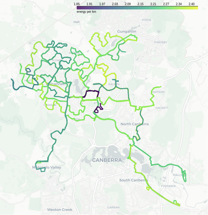
Energy consumption of electric buses serving 18 routes in the Australian Capital Territory in −5.7 °C weather.

Full size image

The dependence of the predicted bus energy consumption as a function of each model variable (with all other variables held fixed at their mean value) is shown in Fig. 3. It is observed that temperature, speed, and gradient have the biggest impact on the predicted energy consumption while average passengers has the lowest. For further discussion of these relationships see the Data-driven Energy Consumption model Section.

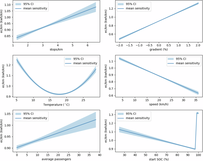
Sensitivity of the predicted energy consumption per kilometre as a function of a single input at a time keeping the other inputs held constant at the data set mean. The shaded area indicates the 95% confidence interval. The bottom right figure shows how batteries are more efficient at higher capacity and that starting trips with close to 100% state of charge reduces opportunities for regenerative braking thereby driving up energy consumption.

Full size image

Energy requirements to service bus schedule

We now move on to considering the electrification of the bus depot servicing these bus routes. The second step is therefore to collate the timetable of routes and calculate the number of buses required to deliver all scheduled services, together with the cumulative energy required by these buses on these routes.

A challenge for the model is that publicly available timetable does not provide information on which bus is operating which routes nor when a bus departs or returns to the depot. Our calculation therefore deals with the aggregate energy required to complete the routes currently being driven (see Method Section for detailed discussion). To once again err on the side of caution we select the busiest week of the annual timetable for our analysis, which in this case is the week of the 4th of April. Figure 4a shows the number of buses required to meet the timetabled schedule as a function of time across the week. At the busiest moment, 85 buses are on the road. Figure 4b shows the amount of energy that the fleet of buses that are on the road will expend on their current routes (before they can next recharge at the depot). The effects of the cold morning weather are evident in the exaggerated peak in energy demand in the morning peak period compared to the afternoon peak period.

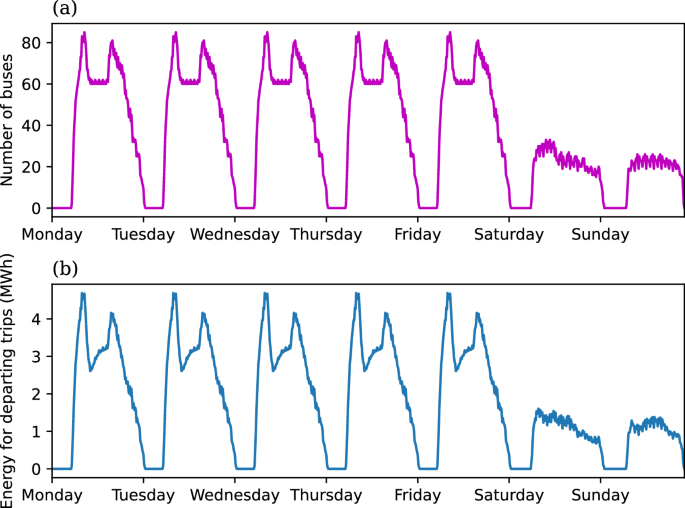
The buses and energy required as a function of time to service the busiest week’s schedule. a gives the number of buses required. b gives the amount of energy that the fleet of buses that are on the road will expend on their current routes.

Full size image

Bus depot charging optimisation

The third step is to determine how to deliver the required electrical energy to the bus fleet, while minimising requirements for costly charging equipment and peak loads on the power grid. We incorporate some practical safety margins into this calculation by adding a dead-running factor onto every trip, and imposing a constraint that buses can only be charged if they are at the depot for an hour or more. We set the dead-running factor to be 10%, which increases the time and energy required for each trip by 10%. As another safety margin, we also enforce that the cumulative state of charge of the bus fleet never drops below 20%.

We assess the impacts on the power grid in two ways. Firstly at the low voltage level by quantifying the peak power the depot draws from the grid at any moment, and secondly at the medium voltage level, by assessing the impact of the depot on the peak load on the zone substation. This second aspect, assessing the depot load in the context of existing loads, is often neglected in modelling^30,31,37, or it is assumed to be included in a price signal from a Distribution System Operator²⁹. We also assess the potential for an onsite battery to contribute towards these goals.

The primary objective of the optimisation algorithm is always to minimise the peak power load of the depot. A secondary objective is to minimise the number of chargers and their power rating, where we specify the available chargers being 300 kW, 150 kW, and 80 kW and that the 300 kW and 150 kW chargers cost proportionately 20 and 5 times as much as a 80 kW charger. Consideration of the effects of the depot on the aggregate zone substation load profile is meanwhile incorporated by prohibiting charging during periods of peak demand.

As the reference case, we assume that buses can be charged whenever they are not on a trip. Figure 5 presents the results for this scenario. Figure 5a shows the number of buses at the depot across the week, together with the number of buses that are free to charge within the constraints of being plugged in for an hour or longer. In this case, this constraint has a minor effect in reducing the available buses.

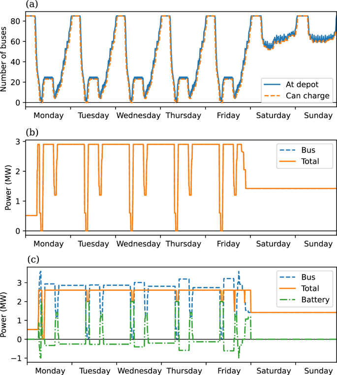
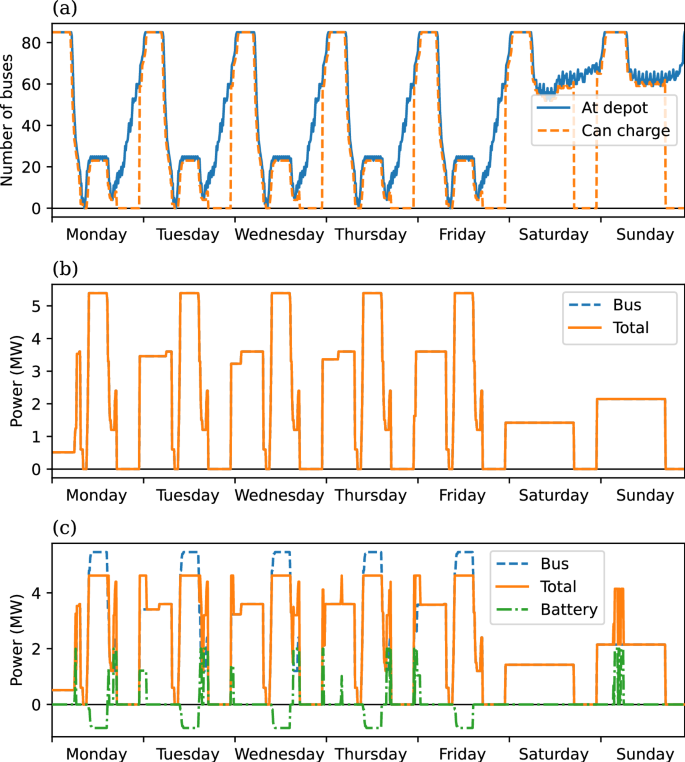
Optimised charging of the bus fleet when charging is permitted at all times throughout the week. a The number of buses present at the bus depot throughout the week (solid line) as well as the subset of buses that are free to charge based on the criteria that they will be at the depot for at least an hour (dashed line). b The electrical load profile in the absence of a depot battery. The total power of the depot (solid line) as well as the power used to charge buses. c The electrical load profiles in the presence of a depot battery. Negative values indicate power being discharged (which only occurs for the battery).

Full size image

Figure 5b shows the optimised charging profile of the aggregate bus fleet at the depot in the case where there is no depot battery. The power load is close to 3 MW throughout most of the work week (Monday to Friday), dipping only at times when most buses are on trips. During the weekend there are far fewer scheduled bus trips so the vast majority of buses are idle and can be charged at a modest rate ahead of Monday. This charging profile can be delivered using 10,300 kW chargers, even though this limits the number of buses charging at any one time to well below the 20 to 80 buses regularly available at the depot (see Figure 5a). The low power consumption during the early morning on Monday is to bring the total state of charge of the bus batteries to 100% (the simulation assumes an equal state of charge at the beginning and end of the week, which is set at 90%).

While the cumulative energy needs of the buses is greatest in the morning (due to cold weather in this worst-case scenario), the charging demand is greatest in the middle of the day when there are only a modest number of buses at the depot that must be quickly recharged ahead of the evening commuting peak.

Figure 5c shows the results for the same scenario as in Figure 5b, except for the inclusion of a 2 MW: 4 MWh battery at the depot. Driven by the objective of the optimisation algorithm to minimise peak demand on the grid, the battery discharges throughout the peak load periods to reduce the peak power by 0.5 MW (to 2.6 MW). This reduction is limited by the energy capacity of the battery, which reflects the flat shape of the charging profile where the energy of the battery needs to be spread across many hours in order to bring down the peak value. The actions of the battery eliminate moments of low power during the day, as the battery utilises the absence of buses at the depot to charge from the grid. While the peak load on the grid is reduced, this configuration regularly provides bus charging at more than 3 MW, which is facilitated by an additional 2300 kW chargers in order to distribute power to a greater number of buses simultaneously. For a more detailed view of the bus charging and battery behaviour, Figure 6 presents the same data as in Fig. 5b, c for the Tuesday.

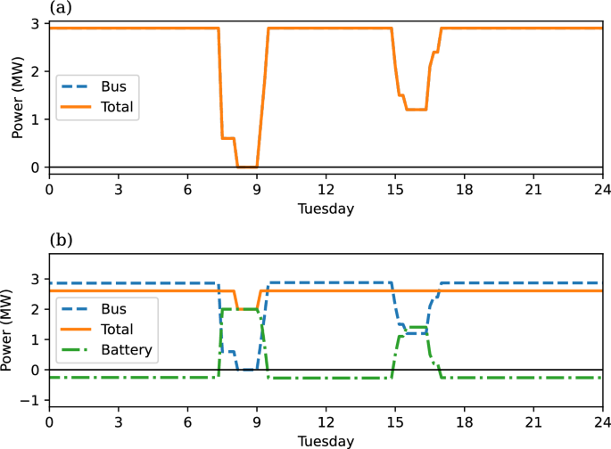
The same data as in Fig. 5 but restricted to showing data only for Tuesday. a In the absence of a depot battery (equivalent to Fig. 5b). b In the presence of a depot battery (equivalent to Fig. 5c).

Full size image

This section modifies the scenario by prohibiting charging (of buses and the depot battery) between 17:00–23:00, which is the period of peak load on the zone substation (as shown in the network provider data⁴⁰). This constraint is the only alteration to the model; the objective function remains the same (it only has fewer hours to work in). The results for the scenario are shown in Figs. 7, 8, mirroring the layout of Figs. 5, 6.

Optimised charging of the bus fleet when charging is only permitted outside of periods of peak demand on the zone substation (17:00–23:00). a The number of buses present at the bus depot throughout the week (solid line) as well as the subset of buses that are free to charge based on the criteria that they will be at the depot for at least an hour and that it is not a period of peak substation demand (dashed line). b The electrical load profile in the absence of a depot battery. The total power of the depot (solid line) as well as the power used to charge buses. c The electrical load profiles in the presence of a depot battery. Negative values indicate power being discharged.

Full size image

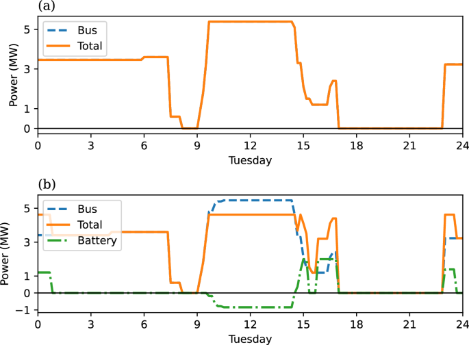
The same data as in Fig. 7 but restricted to showing data only for Tuesday. a In the absence of a depot battery (equivalent to Fig. 7b). b In the presence of a depot battery (equivalent to Fig. 7c).

Full size image

Figure 7a highlights how the constraint on depot charging times significantly reduces the ability to charge buses that are at the depot during the evening time. Delivering the same amount of energy to the bus fleet in a fraction of the time period significantly increases the peak load on the grid. Figures 7b, 8a show that the peak load more than doubles from 2.6 MW to 5.4 MW, due to the pronounced load during the middle of the day ahead of the period of precluded charging – the increase in overnight charging load is more modest. This requires a substantial increase in charging infrastructure, to a total of 18 300 kW chargers and one 150 kW charger.

Due to the more concentrated period of peak load, a battery with the same capacities as before (2 MW : 4 MWh) is able to provide a much greater reduction in peak load of 0.8 MW (down to 4.6 MW), as shown in Figs. 7c, 8b. By distributing the bus charging across a longer time period, the battery also results in reduced charging infrastructure requirements, reducing the number of 300 kW chargers by 4, in exchange for 8 additional 150 kW chargers and one 80 kW charger. These reductions may largely offset the cost of the battery.

Thus far our analysis has focused on the absolute peak load that the depot places on the connection point to the low voltage grid. We now complement this by seeing how these depot load profiles impact the cumulative load on the local (Belconnen) zone substation. This is shown in Figure 9, where the black solid curve shows the current substation load (without an electric bus depot) averaged across the winter months⁴⁰ and the coloured curves show the sum of this current load with the total (bus + battery) depot loads calculated above and presented in Figs. 5–8. Figure 9a presents the data across the week while Fig. 9b focuses on only Tuesday.

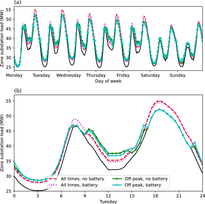
Load on the Belconnen zone substation averaged across the winter months of 2023 (solid black line). The coloured lines show what the load would be with the addition of electric bus depot loads presented in Figs. 5, 7. The dashed and dotted lines give the results when charging is permitted at all times, while the solid lines with markers give the results when charging is prohibited during peak demand periods. The sub-figures share the same legend, which is shown only in b to conserve space in a.

Full size image

Across the four combinations of charging times and batteries there are two clear insights. Firstly, when charging is permitted throughout the day, the depot considerably increases the zone substation’s peak load (by around 3 MW). This remains the case in the presence of a depot battery, which only reduces the impact by 0.5 MW. Given the centrality of peak load to the design and operation of zone substations, this addition could well necessitate extremely costly upgrades. In contrast, the strict prohibition of bus and battery charging during targeted periods completely prevents additions to peak load and instead leads to increased utilisation of the existing power rating of the substation throughout non-peak periods of the day.

The second take away is that the impact of the depot battery is, in the scheme of the zone substation, modest. This is understandable given the scale of the battery (2 MW) compared to the total load on the zone substation (>50 MW) and the total load of charging the bus fleet (>5 MW). The greatest impact of the battery on the load profile shape is to increase the morning peak load, as the battery charges while most buses are on morning trips. This peak remains lower than the evening peak load so this may, or may not, be a problem. Interestingly prohibiting charging during the evening peak also stops the battery from adding this morning load. This is because the depot’s peak load during the middle of the day is so large that the battery can’t achieve any impact on peak demand by discharging during any other times of the day and therefore doesn’t need to charge as much.

The above analysis utilised a fixed battery capacity (2 MW: 4 MWh), which was found to have only a modest impact on the depot on the low voltage connection point and an even more limited impact on the zone substation. In this last section we investigate how varying the power and energy capacity of the battery effects its ability to reduce the peak load. In this we focus on the metric of peak load at any time of the week, noting that all the insights on correlation with zone substation load hold irrespective of battery size.

Figure 10 shows the peak load across a range of battery power and battery energy capacity combinations. Figure 10a is when charging is permitted at all times, while Fig. 10b is when charging is prohibited during peak periods. The trends are seen to be similar in both cases, with the peak loads predominantly dependent on the x-axis. This corroborates the developed intuition that the energy capacity of batteries is the limiting factor due to the flat, spread-out shape of the optimised bus charging load profiles. The absolute value of the impact is greater for the time-restricted charging profile as the bus charging profile is concentrated into fewer hours where the battery focuses its finite energy capacity.

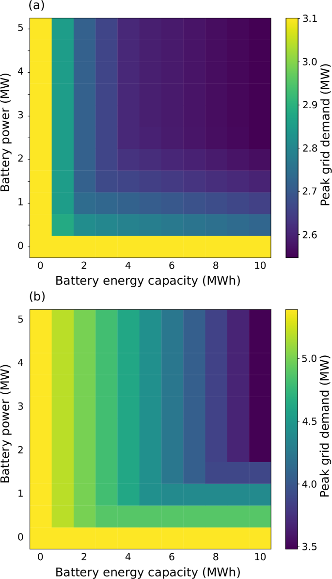
Bus depot peak load as a function of an on-site battery’s energy capacity (x-axis) and power rating (y-axis). a When charging (of buses and the battery) is permitted at all times throughout the week. b When charging is prohibited during periods of peak load on the zone substation.

Full size image

The presented case study demonstrates the power of an integrated model of electric bus energy consumption and depot bus charging that needs as inputs only publicly available data. Such a model enables users, including researchers and transport industry practitioners, to quickly study specific routes and regions of interest without the need for any bespoke field data.

The energy consumption model can be used to determine what the most challenging conditions will be for the electrification of the relevant routes based on the impacts of local topology, temperature, and traffic. These location-specific needs are then incorporated into the bus fleet charging model, which we showed gives an indication of the optimum charging infrastructure that will minimise the peak load placed on the power grid, and how both the peak load and charging infrastructure can be affected by a depot battery.

One application of the tool, which we know transport departments and bus operators are using it for, is to survey a set of routes and depots to ascertain which may be electrified most easily and economically. This is emerging as a high-impact field of research¹² and industry activities. RouteZero is particularly adept for this process of quantifying and communicating the integration between power grids and electric mobility systems for non-experts in power grids.

One specific aspect of the integration of these (physical and socio-economic) systems that was highlighted in the case study is the possibility for tensions between reducing power demand at the depot’s grid connection point and reducing peak demand on the zone substation (and generally at the higher levels of the power grid). Traditionally distribution network operators and regulations focus on the connection point. However, as we’ve seen, electric bus depots have such large and flexible loads that factoring in considerations of loads throughout the higher levels of the power grid could lead to more globally optimal results. This would require collaboration between mobility and power grid stakeholders. Particularly as our results showed that prohibiting charging during certain periods can dramatically increase the charging infrastructure required to service the bus schedule as well as the loads on the depot connection point, both of which will incur costs on the depot operator. Avoiding periods of peak network loads, on the other hand, may be avoid peak network demand charges.

A limitation of the model, as currently available to users, is the data used to fit the bus energy consumption model has a limited range and has less than ideal fidelity (details in Method Section). This cautions against use for vastly different conditions. This limitation would be straightforward to address if users have access to a more comprehensive data set, to which the open-source method could be applied. Another aspect for future work is to extend the optimisation to total costs – adding operating costs such as network demand charges and electricity market prices, which vary significantly between locations – to find the optimal infrastructure arrangement.

Finally, we reiterate that research indicates that the electrification of buses and depots can benefit substantially from, and can create additional benefits if, bus routes and schedules are redesigned around the specific capabilities of electric buses^10,13,14. While RouteZero is designed to easily simulate the electrification of fixed bus routes and schedules, it could be applied to redesigning these if users inputted their redesigned routes and timetables in the GTFS format.

This section summarises the method of the bus energy consumption model and the bus depot charging optimisation. Detail on the software implementation and webapp use are provided in⁴¹.

Data-driven energy consumption model

A Bayesian linear regression model is fit to the modelling data. We choose a linear regression model because of its ease of interpretation, lower dependence on large amounts of data when compared to non-parametric models such as random forests and neural networks, and greater ability to extrapolate outside the training data. A Bayesian approach is used to fit the model as it quantifies the uncertainty in the parameter values. This allows a confidence interval to be placed on the predictions.

The linear regression model can be represented as

where e is an error term that is approximated as zero-mean Gaussian and I_>97% is an indicator function that indicates if a trip is started with a close to full battery:

These are summarised in Table 1, which also presents their values as fit to the trial data.

Several variable transforms have been included: temperature squared, and a battery close to full indicator. These account for the following patterns.

Energy consumption by auxiliary systems (air conditioning and battery management) has an approximately quadratic relationship with the external temperature²³. ec/km as a function of SOC_i has a clear negative trend—batteries are more efficient at higher capacity—with the exception that at close to 100% initial state of charge the trips have a much higher energy consumption. This is explained by ref. ²³ as a result of less ability to regeneratively brake if the battery is already close to full. To model this the indicator function, I_>97% is used.

The data set was split 80/20 into training and validation sets. The model parameters were fit to the training data using Bayesian linear regression²⁸. Briefly, given output ({bf{y}}in {{mathbb{R}}}^{n}), inputs ({bf{X}}in {{mathbb{R}}}^{ntimes p}), model parameters ({boldsymbol{theta }}in {{mathbb{R}}}^{p}) with a zero-mean Gaussian prior such that

where e is zero-mean Gaussian with covariance Σ, then the parameters will have posterior mean and variance given by

where Σ_p is the prior covariance of the parameters.

This was used to fit our linear regression model with a large prior covariance placed on the parameters to represent no prior knowledge and the measurement variances.

To develop a data-driven predictive model for electric bus energy consumption a training dataset of bus trips was required. Where for each trip the input (independent) and output (dependent) parameters wishing to be modelled are recorded. The required data was collated from several sources: Zenobe, Transport for NSW, and publicly available temperature and weather data. The collected data corresponds to the battery electric bus trial at the Leichhardt bus depot in Sydney’s inner west as part of the Next Generation Electric Bus Depot Project²⁷. The data from these sources were cleaned, combined, and processed to give the following information about each trip undertaken by a bus on a route:

• average gradient (%),

• average number of passengers,

• number of stops per kilometre,

• average speed (km/hour),

• starting battery state of charge (%),

• temperature (degrees Celsius),

• energy consumption per kilometre (kWh/km),

• distance (km),

This final data set contains no information about road condition, and driver aggressiveness, and all vehicles in the trial have the same mass. As such, these variables were excluded from the modelling. Road condition was excluded as all the modelling data was collected in Sydney’s inner west and so a range of different road conditions would not be present.

After processing, the final dataset spanned the time-frame from 6th of of January 2022 till the 31st of August 2022 and consisted of 10459 trips on 42 different routes by 33 different buses. Table 2 summarises the variables contained in the dataset and the distribution of the variables in the dataset is shown in Fig. 11.

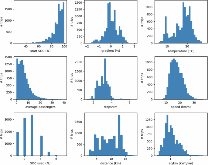
Both the dependent (output) and independent (input) variables are shown. Also shown is the distribution of the percent state of charge used on trips and trip distance from which the energy consumption per kilometre is calculated.

Full size image

It can be seen that several of the input variables cover only a limited range. The majority of trips have:

• a moderate temperature between 7 °C and 26 °C,

• a relatively flat average gradient between −1.8% and 1.8%,

• a higher stop per kilometre ratio > 2,

• a lower average speed < 30 km h⁻¹.

These limited ranges are in line with the time of year the data was collected and the location and types of routes it corresponds to Sydney’s inner west.

The fit parameter means and 95% confidence intervals are given in Table 1. The model was validated by making predictions on the validation set and calculating the prediction error, which had a weighted mean of 5.34 × 10⁻³ kW h km⁻¹ and a standard deviation of 0.278 kW h km⁻¹.

Given that the error introduced by recording the state of charge in integers has an average standard deviation of approximately 0.279 kW h km⁻¹, we can be confident that the trained model is the best that can be achieved given the dataset.

Static General Transit Feed Specification (GTFS) files are used as the primary source of data when producing outputs for an end-user. Files containing information about a large number of routes within Australia are freely available online for each state and territory. A summary of the contained data relevant to the modelling is given below. A detailed description of the data in the online reference documentation²⁵.

For each bus route the GTFS files give the following information:

• the trips schedule on this route,

• a list of stops belonging to the route and their locations,

• the arrival and departure time of each bus stop on a trip,

• the stops along the route and their locations,

• a GPS path for the route.

Added to this is temperature and elevation information obtained from public sources and passenger information provided by the end-user.

From this, the inputs required for the electric bus energy consumption model (see the Data-driven energy consumption model Section) are calculated allowing predictions of energy consumption to be made. A schedule of trips for a selection of routes can also be extracted which is used in the depot charging optimisation model (see the Depot charging optimisation model Section).

Depot charging optimisation model

The objective is to find the charging profile that minimises the required grid connection power and a number of chargers while ensuring that the buses are sufficiently charged to service the route timetable. Care has been taken when formulating the objective and the constraints to ensure the problem is formulated as a linear programme that can be solved efficiently in polynomial time⁴².

Let G be the grid connection power limit, and N_c be the number of chargers. For a given time window t, the amount of charging done is x_t, the depot battery power is b_t, and r_t is an auxiliary variable introduced to minimise changes in power. Additionally, s_f, and s_r are slack variables included to ensure a feasible solution. With these defined the linear programme that we wish to optimise is

where θ = {G, N_c, x_t, b_t, r_t, s_f, s_r∣ ∀ t = 1, . . , T} is the set of all optimisation variables, which are outlined in Table 3. Q is a large cost placed on the slack variables to ensure the constraints will be satisfied if feasible, p₀ is a cost used to minimise the required grid connection capacity, p₁ is a smaller cost placed on the number of chargers.

The inclusion of x_t + b_t and r_t in the objective acts similarly to regularising the charging power (i.e. similar to placing a quadratic cost on power) while maintaining the linear nature of the problem. In essence, p₂ is a small cost placed on charging power to prevent unnecessary charging, and the auxiliary variable r_t is included to minimise large changes in the charging power. This is done by including a constraint to ensure it is greater than the absolute difference in charging between two consecutive time steps:

The following constraint is used to limit the amount of bus charging done based on the number of buses at the depot, N_t, and the number of chargers:

where a_t is a binary variable indicating whether the user has allowed charging during this time period, U_x is the lesser of the maximum charger power rating or the maximum bus charging power. The grid connection constraint is enforced by

Enforcing that the cumulative charging done is less than the cumulative energy used by buses that have returned to the depot plus the gap between the starting capacity and max capacity. That is, ensuring the state of charge is less than the maximum:

where α is the constant converting from kW to kWh, C_s ∈ (0, 1] is the starting charge ratio, M is the number of buses, B is the bus battery capacity, L ∈ (0, 1] is the end of life battery battery capacity as a ratio of rated battery capacity, η_x is the bus charging efficiency, and E_r,t is the energy used on trips returning in time period t. The end of life battery capacity needs to be considered as battery health degrades over time resulting in decreased energy capacity and this should be considered when determining if the capacity is sufficient.

Enforcing that the cumulative charging done is greater than the cumulative energy required by buses that have departed the depot minus the difference between the start state of charge and the reserve. That is, ensuring that the state of charge is above the reserve:

where R is the required reserve capacity, E_d,t is the energy required by trips departing in time period t, and the slack variable s_r ≥ 0 is included to ensure an optimisation solution is reached even if the reserve cannot be achieved.

Enforcing the desired final state of charge is achieved:

where C_f ∈ (0, 1] is the required final charge ratio, the slack variable s_f ≥ 0 has been included to ensure that a solution is reached even if the desired final state of charge cannot be achieved.

Minimum plugin time constraint, i.e. enforces that during the specified number of time windows a single charger cannot charge more than the battery capacity of a bus:

Note, that this only approximates the desired constraint as we cannot know how much capacity each bus has used.

For the on-site depot battery we define η_b as the charge and discharge efficiency, and D as the capacity. This allows the on-site depot battery minimum, maximum and final state of charge constraints to be formulated as follows.

Battery charging and discharging efficiency introduce a piecewise linear function of the form

A standard implementation of this might involve the introduction of binary variables resulting in a mixed integer programme and drastically increasing the computational complexity. To avoid this, we follow a standard reformulation of piecewise linear problems as a linear problem⁴³ introducing the auxiliary variable v_t:

This auxiliary variable can be thought of as the power applied to the battery after the effects of efficiency have been considered. Here, inequality constraints can be used in the reformulation as the objective function ensures that the solution for v_t will lie on the constraint boundary.

The battery minimum, maximum, and final state of charge can now be enforced by

The complete optimisation model describes a linear programme that can be solved efficiently using the open source CBC library from COIN-OR⁴⁴.