An integrative phenotype-structured partial differential equation model for the population dynamics of epithelial-mesenchymal transition

Introduction
Intra-tumour heterogeneity—the co-existence of multiple distinct cellular phenotypes in a tumour—is being increasingly reported to associate with poor patient outcomes. It contributes to both metastasis and therapy resistance—two major unsolved clinical challenges1,2. Such heterogeneity can arise at a genetic level over the course of tumour evolution and manifests as different clonal populations3,4,5. However, over the last two decades, non-genetic or phenotypic heterogeneity among cancer cells has been identified as a key driver of disease aggressiveness6,7,8,9. Such heterogeneity is often characterised by single-cell measurements (flow cytometry, mass cytometry, RNA-seq, ChIP-seq, ATAC-seq), showing diversity among cells in a population at the proteome, transcriptome and epigenome levels. A canonical example of non-genetic heterogeneity is along the Epithelial-Mesenchymal (E-M) phenotypic states in carcinomas10,11. E-M heterogeneity has been implicated in poor patient prognosis, and several in vitro and in vivo studies have shown its contribution to cancer metastasis and drug resistance12,13,14,15. Thus, understanding cellular mechanisms driving E-M heterogeneity can help improving therapeutic outcomes.
An iterative interplay among in silico and in vitro studies has contributed enormously to deciphering how non-genetic heterogeneity emerges in a population. Mathematical modelling of regulatory networks underlying Epithelial-Mesenchymal Plasticity (EMP) have reported the co-existence of multiple cellular phenotypes—Epithelial (E), Mesenchymal (M) and one or more hybrid E/M (H) cell states16,17,18,19,20. Their co-existence has been experimentally reported in varying ratios in multiple cell lines and primary tumours10,21. Synthetic perturbation of the underlying regulatory network led to the loss of bimodal nature of canonical epithelial markers such as E-cadherin and altered the phenotypic distribution12,13,22,23. The relative stability of cells in different phenotypes, and consequently the phenotypic distribution of the population at a given time is governed by alternative, self-reinforcing network interactions between epithelial and mesenchymal players in the gene regulatory network24. The epigenetic regulation of genes further reinforces transcriptional state. Happening at timescales slower than transcriptional regulation, the epigenetic regulation can be reversible or irreversible, as observed experimentally. Thus, epigenetic remodelling can lock cells transiently or permanently in a cell-state, impacting the population phenotypic distribution25,26. Further, cell-to-cell communications either through neighbourhood interactions or paracrine signalling also reshapes the phenotypic distribution27,28,29,30. Hence, a diversity of regulatory interactions within and among cells can contribute to shaping the E-M heterogeneity patterns in a cell population.
Another set of factors such as asymmetric cell division31,32, stochastic biochemical noise33, differences in cellular microenvironment34 and variable cell-cycle dynamics35 can amplify dynamic heterogeneity in a cellular population. These factors alter cell-to-cell variability in protein levels in a population, thus contributing to their functional heterogeneity (differential activation of signalling pathways) when these cells are exposed to cytotoxic or EMT-inducing growth factors36,37. Despite extensive efforts in investigating above-mentioned regulatory and stochastic processes in E-M plasticity and heterogeneity, only a few computational models have incorporated these processes within a growing and dividing heterogeneous cellular population.
In the present work, we use Cell Population Balance modelling to study the dynamics of E-M heterogeneity in a growing cell population, relying on partial differential equations (PDEs). In general, Cell Population Balance models capture the evolution of the cell density given the regulatory, stochastic, and population dynamics of cells without dealing with individual cell level information. Our Cell Population Balance model combines three main cellular processes: (1) growth due to cell division and cell death, (2) state regulation, which corresponds to the time-evolution of the regulatory molecules defining a cell’s phenotype, based on corresponding ODE models and (3) stochastic cell transition, which aggregates all sources of stochasticity in the fate of a cell’s phenotype.
With the developed model, we explore how heterogeneity along the E-M axis emerges at a population level. We first show that the Cell Population Balance model can capture the previously reported dynamical features of hysteresis, and epigenetic regulation during cells undergoing an Epithelial-Mesenchymal Transition (EMT) followed by a Mesenchymal-Epithelial Transition (MET). Next, with the full model incorporating state regulation, cell growth and transition, we report that increasing biochemical noise in regulatory molecules can enhance E-M heterogeneity given that the regulatory network operates in the multi-stable phenotypic regime. On the other hand, E-M heterogeneity can also be lowered down because of differences in subpopulations growth rates. Further, for an abrupt change in E-M phenotypic composition of a population, the timescale of re-equilibration depends on the rate at which intra-cellular constitutive EMT signal (here, SNAIL) re-equilibrates. And lastly, we show that resource competition for cellular growth among E-M subpopulations can give rise to biphasic growth or initial phenoptypic composition dependent steady state E-M heterogeneity.
For all simulations, we use a scheme from the family of particle methods, based on solving a properly defined set of ordinary differential equations (ODEs)38. These are particularly adapted for models based on PDEs such as those developed in the present paper. For the derivation and analysis of particle methods in that context, we refer to the recent theoretical work39, where it is proved that solutions are properly approximated by the proposed numerical method.
Results
Development of a general Cell Population Balance model capturing cell state regulation, cell growth and cell state transition
In this work, we aim to describe a large population of cells which are characterised by their phenotypes. More precisely, for each cell, the quantity (yin {{mathbb{R}}}^{n}) represents the concentration of several different (internal or external) molecules associated with the cell. Here, n represents the dimension of the phenotypic space, that we will also refer to as ‘state space’. The dimension n of the phenotypic space will then correspond to the number of different molecules that determine the phenotype of each cell. With this approach, the evolution of a population of Nc cells can be described by a system of Nc coupled Ordinary or Stochastic Differential Equations, giving the evolution of each cell’s phenotype y(t). As a consequence, the number of equations to be solved grows with the number of cells in the population, and such a model can rapidly give rise to costly simulations.
Another approach, usually referred to as macroscopic or continuous approach, consists of focusing on the cell density instead of tracking the evolution of each individual cell’s phenotype. The cell density that we will denote by u from here onwards, is then a function of the phenotype y and of time t. More specifically, for each subset (Omega in {{mathbb{R}}}^{n}) of the phenotypic space, the quantity ∫Ω u(t, y)dy represents the number of cells whose phenotype belong to Ω at time t. The evolution of the cell density u is described by a Cell Population Balance model, which is, mathematically speaking, a PDE. This approach is known to be a good approximation of the microscopic model when the number of cells is large.
To give an intuition for the final PDE model, we consider a simplified case, in which a cell’s phenotype is assumed to be determined by the concentration of one given molecule, so that the phenotypic space is one-dimensional (n = 1). The function u is to be understood in the following way: for any phenotype interval [a, b], the integral (mathop{int}nolimits_{a}^{b}u(t,y),dy) represents the number of cells whose phenotype belongs to [a, b]. Thus, the total number of cells is computed by ({int}_{{mathbb{R}}}u(t,y),dy), which will be denoted by ρ(t). In our model, the total number of cells ρ(t) is amenable to evolve in time.
Three mechanisms will be considered to participate in increasing or decreasing the number of cells within each interval [a, b]: growth, cell regulation and stochastic state transition. Their interplay is illustrated in Fig. 1 and individual descriptions are provided as follows:

In each panel, the cell density u is represented at time t in black, and at a subsequent time t + Δt in colour. The number of cells with cell state in the interval [a, b] is represented by the hashed (black or coloured) area. Growth (which includes cell division and cell death) results in an upward or downward shift of the cell density. In this toy example (top left panel), cell division takes place faster than cell death, so the cell density at time t + Δt is shifted upward compared to the cell density at time t. Consequently, the number of cells with cell state in [a, b] increases between t and t + Δt. State regulation results in a horizontal displacement of the cell density. In this example (center left panel), a concentration phenomenon is taking place towards the center of the state space. Here, the number of cells with cell state in [a, b] increases between t and t + Δt. Stochastic state transition leads to a mixing of the cell population. The evolution of the number of cells with cell state in [a, b] depends on the cell density at every other point of the state space. This results in a diversification of the population, that is in a flattening of the cell density curve (bottom left panel). In this example, the number of cells with cell state in [a, b] decreases between t and t + Δt. All three mechanisms combine in the cell population balance model to give the evolution of the cell density (right panel).
The first mechanism that we include in our model is ‘State Regulation’. At the level of a single cell, the evolution of its phenotype y(t) is assumed to be given by the following ODE:
where (dot{y}) denotes the derivative of y with respect to time.
We extrapolate this simple ODE model to describe the evolution of the cell density of a whole population. In the PDE framework, the so-called advection term accounts for all cells whose phenotypes will enter or leave the phenotypic region [a, b] during a small time interval as a result of their inner evolution. Taking only this mechanism into account, the variation of the number of cells in the region [a, b] between two time instants t and t + Δt is computed as:
The sign of f at points a and b determines whether cells enter or leave the region. For instance, if f(a) > 0, the first term of the right-hand side is positive, which translates the fact that cells enter the region [a, b] at point a. Similarly, if f(a) < 0, cells leave the region [a, b] at point a. On the other hand, if f(b) > 0, cells will leave the region [a, b] at point b, and if f(b) < 0, cells will enter the region [a, b] at point b. Intuitively, cells will then be transported towards the right when f is positive, and towards the left when f is negative. Concentration phenomena will happen at points where f is zero and has negative derivative: these points are asymptotically stable points for the ODE (dot{y}=f(y)). Figure 1 illustrates a toy situation in which f has a stable equilibrium point towards the middle of the phenotypic space, resulting in concentration of the cell density around this point (Fig. 1 left middle panel).
We also choose to take into account population growth, which includes cell division and cell death. Each cell of phenotype y divides at rate r(y) and its daughter cells are assumed to be given the same phenotype y. Hence, the quantity of new cells at time t + Δt with phenotype in [a, b] is given by (Delta tmathop{int}nolimits_{a}^{b}r(y)u(t,y),dy). Cells are also assumed to die at a rate d(y)ρ(t), proportional to the total number of cells (rho (t)={int}_{{mathbb{R}}}u(t,y),dy). The quantity of cells that died between the times t and t + Δt is then approximated by (Delta tmathop{int}nolimits_{a}^{b}d(y)rho (t)u(t,y),dy). The term ‘r(y) − d(y)ρ(t)’ thus represents the net growth rate, where r(y) is the division rate, and d(y)ρ(t) the death rate. It is positive if cell division is faster than cell death, and negative in the opposite case. Overall, the evolution of the number of cells between times t and t + Δt caused by the cell population growth is given by
Depending on the sign of the right-hand side, the growth mechanism will result in an upward or downward vertical shift of the curve representing the cell density (see Fig. 1, top left panel).
The third mechanism that we take into account is ‘stochastic cell-state transition’, that we will also refer to as cell-state transition. Here, M(y, z) represents the (infinitesimal) probability that a cell’s phenotype z changes to a phenotype y. Thus the number of new cells with phenotypes in the interval [a, b] at time t + Δt is computed as (Delta tmathop{int}nolimits_{a}^{b}({int}_{{mathbb{R}}}M(y,z)u(t,z),dz),dy). Symmetrically, the number of cells whose phenotypes were in [a, b] at time t and who mutated between times t and t + Δt is computed by (Delta tmathop{int}nolimits_{a}^{b}({int}_{{mathbb{R}}}M(z,y),dz),u(t,y),dy). This mechanism is fundamentally non-local, in that the evolution of the number of cells with phenotypes in the interval [a, b] depends on the whole cell population. Often, this mechanism results in a mixing of the population, that is in a flatter cell density (as illustrated in Fig. 1, bottom left panel).
Putting everything together, the variation of cells whose phenotype belongs to [a, b] during a time interval Δt is approximated by
The combination of the three mechanisms is illustrated in Fig. 1 (right panel).
It is worth stressing that, all in all, we obtain a model where the interaction between cells happens solely at the level of the growth term. It is mediated by the non-local logistic term involving the total population size ρ(t).
Taking the limit Δt going to zero in Equation (2), we obtain a PDE modelling the mechanisms of advection, growth and cell-state transition. Generalising to any dimension n, it can be written as
and then complemented with an initial condition describing the density of cells at time 0.
Incorporating EMT state regulation in the developed model captures hysteresis in EMT-MET cycle, and delayed MET after prolonged EMT induction
We first focused on the case where cell-state transition and growth in (5) are neglected. In this case, equation (5) reduces to the so-called advection equation (also often named transport equation), namely
This equation is the exact PDE analogue of the ODE
In vitro and in silico studies on EMP have demonstrated two specific dynamic phenomena as cancer cells undergo one cycle of EMT and MET:
-
1.
Asymmetry in EMT and MET trajectories (hysteretic behaviour) of cell states.
-
2.
Delayed MET with an increasing duration of EMT inducer treatment due to epigenetic (chromatin-based) stabilisation of M and H states.
To properly define the advection function f underlying state regulation, we chose a minimal EMT regulatory network with canonical epithelial (microRNA-200 (miR-200)) and mesenchymal (mRNA ZEB) players that mutually inhibit each other via transcriptional and translational regulation. An EMT-inducing transcription factor SNAIL that activates ZEB and inhibits miR-200 represents the cumulative effect of upstream signalling pathways40. The corresponding ODE model is given by
This ODE system is the modelling core for the advection term in all our simulations. It will progressively be made more complex in the corresponding section, or approximated by a simpler model to ease the computational burden when necessary (see next section). All the corresponding parameters are given in ‘Parameters for ODE (8) and (9)’.
We denote F = F(μ200, Z, S) the right-hand side of this ODE model, which accounts for interactions between a transcription factor ZEB (denoted Z), and a micro-RNA miR-200 (denoted μ200). The variable S represents a third molecule, SNAIL, which is seen in our case as an external signal characterising the extracellular environment. Note that this model falls into the framework introduced in equation (7), considering that y is the vector of miR-200 and ZEB concentrations y = (μ200, Z), and taking f(t, y1, y2) = F(μ200, Z, S(t)).
The bifurcation diagram (Fig. 2A) depicts the different possible stable states, each characterised by a specific range of miR-200 levels (solid lines) for increasing levels of SNAIL, resulting from the network dynamics (8). As a cell undergoes EMT (i.e. SNAIL levels increase), it switches from high to intermediate to low levels of miR-200 which corresponds to E, H and M state respectively. However, during MET, the cell switches directly from low (M) to high (E) miR-200 levels, thus displaying hysteresis.
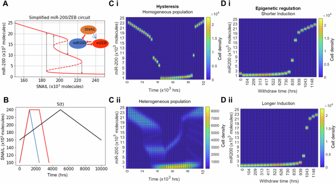
A EMT gene regulatory network (inset) and the bifurcation of cell states resulting from the network dynamics with increasing input signal (SNAIL) levels, B Variation in the external input (SNAIL) levels with time to capture hysteresis and epigenetic regulation of cell states in (C, D). C Hysteresis (non-symmetric trajectories) in cell state transition during one cycle of EMT and MET by varying SNAIL levels (black curve) as shown in (B) while considering—(i) Homogeneous population and (ii) Heterogeneous population. D Dynamics of miR-200 levels in homogeneous population during withdrawal of SNAIL levels post short-term (i) and long-term (ii) EMT induction (blue and red curve in B, respectively). Growth of cells and state transition because of biochemical noise are neglected in these simulation results.
To reproduce the hysteretic behaviour of EMP, i.e. asymmetry in EMT and MET trajectories, we first simulated the advection equation (6) associated to ODE (8). In other words, we are considering (6) where y = (μ200, Z) is the two-dimensional vector of miR-200 and ZEB concentrations, the advection function is given by f(t, μ200, Z) = F(μ200, Z, S(t)), and t ↦ S(t) is the piecewise-linear function which connects the points (0, 160K), (5000, 240K) and (10,000, 160K), as represented in Fig. 2B (black; here K represents 103 molecules).
We confirmed that the Cell Population Balance model developed here captures hysteresis, upon using SNAIL dynamics shown in black curve (Fig. 2B). For a homogeneous cell population (Fig. 2C, i), we see that the cells reside in three distinct miR-200 states (high, intermediate, and low) for time 0–5000 h (increasing SNAIL levels), but make a quick transition from low to high miR-200 levels for time 5000–10,000 h without spending much time in the intermediate state (decreasing SNAIL levels). The intermediate miR-200 levels seen during MET are to be understood as a sample timepoint where miR-200 levels are responding to changes in SNAIL levels before settling to their equilibrium (high) state.
In order to account for heterogeneity within the population, and more specifically for the fact that the signal S can be interpreted in a different way by each cell, we incorporated S within the structure variable, which becomes y = (μ200, Z, S). SNAIL level variation then impacts the advection term, which becomes f(t, y) = (F(y), fS(S)), where fS is the step function corresponding to the derivative of the function S introduced in the previous paragraph, i.e. fS(S) = 40 if S ∈ [0, 5000), and fS(S) = −40 if S ∈ (5000, 10,000]. As initial condition, we considered a population homogeneously distributed in the molecules ZEB and miR-200, but with heterogeneous levels of SNAIL distributed according to a truncated Gaussian. In other words, we let ({u}^{0}({mu }_{200},Z,S)=frac{1}{sigma }Gleft(frac{S-{S}_{0}}{sigma }right){{mathbb{1}}}_{[50K,250K]}(S){{mathbb{1}}}_{[0,25K]}left({mu }_{200}right){{mathbb{1}}}_{[0,1K]}(Z)), where S0 = 160 K, σ = 20K and G denotes the Gaussian function, i.e. (G(x)=frac{1}{sqrt{2pi }}exp (-{x}^{2}/2)).
In this case, we obtain hysteresis as well (Fig. 2C, ii). Particularly, the cell distribution along ZEB and miR-200 axis during MET shows that the transient intermediate miR-200 peak in homogeneous population has turned into little dispersed transient peaks which were clearly distinct from the intermediate peak arising during EMT (Fig. S1). This observation corroborates with the experimental data on different partial states seen during EMT vs. during MET10. Also, in the heterogenous population case, some cells fail to complete a full EMT, rather undergo a partial transition and then return to an epithelial state upon reduced SNAIL levels (Fig. 2C, ii).
The range of SNAIL values for which E, H and M states are stable (Fig. 2A) can be altered by epigenetic (chromatin-based) changes that can happen during long-term EMT induction, leading to a delayed MET41,42. Therefore, to capture this phenomenon within our modelling framework, we incorporated the phenomenological formalism to account for epigenetic changes in EMT regulatory network (equation (9),43). In order to do so, we considered the ZEB’s threshold for inhibiting miR-200, ‘Z0’, to be a time-dependent variable such that the longer ZEB remains in the high states during EMT, the lower Z0 becomes. This lowered Z0 value enables ZEB’s inhibition of miR-200 to continue even if ZEB level goes down when the external inducer is withdrawn42,43,44. To incorporate this phenomenological approach to model epigenetic regulation in the model, we correspondingly augmented the structure variable, which becomes y = (μ200, Z, Z0, S). The considered advection function is that associated to the ODE:
All corresponding parameters are detailed in ‘Parameters for ODE (8) and (9)’. Denoting Fe the right-hand side of this ODE, the corresponding PDE model (6) has advection function given by fe(t, μ200, Z, Z0, S) = Fe(μ200, Z, Z0, S(t)). In a first simulation (Fig. 2D i), S is the piecewise-linear function which connects the points (0, 100K), (1200, 240K) and (2400, 100K), as represented in Fig. 2B (blue curve), and in a second simulation (Fig. 2D ii), the piecewise-linear function which connects the points (0, 100K), (1200, 240K) and (2400, 240K) and (3600, 100K) (red curve in Fig. 2B).
We considered two SNAIL levels dynamics to show the influence of epigenetic changes during EMT: Short-term induction (Fig. 2B blue curve), and Long-term induction (Fig. 2B red curve). We see that homogeneous cell population have longer recovery time for long-term EMT induction than for short-term induction, therefore, recapitulating the previous observation based on population’s average cell analysis43.
Incorporating E-M subpopulations’ cell growth and spontaneous state transition in the Cell Population Balance model
We then moved on to considering the full model (5). In this case, precise models for the functions underlying the growth and cell-state transition terms are not as established (or even missing), making our approach more qualitative than quantitative.
When incorporating growth and cell-state transition into the model, computation times become prohibitive. We hence used dimension reduction by further simplifying the advection function: we considered the state y = (x, S) rather than (μ200, Z, S), where x is roughly equivalent to μ200, as explained below.
This requires to choose a function fr such that the dynamics of x for any S is given by (dot{x}={f}_{r}(x,S)). Our main requirement in choosing this new function is to preserve the bifurcation diagram given in Fig. 2A, which means that, for a given value of S ∈ [150K, 250K], fr(⋅ , S) has the same number of zeros as F(⋅ , S), and are such that fr(x, S) = 0 if and only if there exists Z > 0 such that F(x, Z, S) = 0.
Since infinitely many functions satisfy this property, one must make further assumptions in order to select a suitable one. For simplicity and to avoid overfitting, we assumed that, for any S, fr(⋅ , S) is piecewise linear (with one root per interval where it is linear) and that the rate of change is constant on each interval. Under these constraints, the function is defined up to a multiplicative constant which is chosen by minimising a suitably defined criterion, see ‘Reduction of the advection function’.
Figure S2 A shows the shape of the function x ↦ fr(x, S) underlying the reduced ODE for different values of S, and highlights the relative stability of possible cell-states for increasing levels of input S.
After reduction, and considering now growth and cell-state transition, the full PDE model incorporating growth and stochastic state transition is of the form (5) in dimension n = 2, namely
where:
-
The structure variable (yin {{mathbb{R}}}^{2}) is y = (x, S).
-
The advection function f is given by f(y) = f(x, S) = (fr(x, S), fS(S)), where
$${f}_{S}(S)=delta left(1-frac{S}{{S}_{0}}right),$$(11)with S0 ∈ [150K, 250K] corresponding to the mean of the SNAIL distribution, (delta :=frac{{S}_{0}ln (2)}{alpha }), and α > 0 representing the characteristic time of convergence of SNAIL to the mean S0.
-
Within the term (left(r(y)-d(y)rho (t)right)u(t,y)) representing the net growth of cells of state y, the death rate is always considered to be independent of the cell state (i.e. d(y) = d≡1.82 × 10⁻⁷cell/h, as in ref. 32).
-
The ‘mutation’ function M is taken to be (M(y,z)=r(z)P(y-z){{mathbb{1}}}_{[0,25K]times [150K,250K]}(y)). This choice is motivated by the assumption that transitions occur at cell division. We note that other modelling assumptions might lead to the same choice. The presence of indicator functions ensures that the support of the solution remains in the rectangle [0, 25K] ×[150K, 250 K] at all times. Here, (P(y)=P(x,S):=frac{1}{{eta }_{x}{eta }_{S}}G(frac{x}{{eta }_{x}})G(frac{S}{{eta }_{S}})), where G is the Gaussian function. Hence, a cell defined by state x, S gives birth to daughter cells defined by state ({x}^{{prime} },{S}^{{prime} }). Our models captures how far ({x}^{{prime} }) and ({S}^{{prime} }) are from x, S through standard deviations ηx and ηS, respectively.
To solve (10), we make use of a particle method adapted to this problem, as introduced in ref. 39. The details of this numerical method are given in ‘Numerical method’.
Biochemical reaction noise, coupled with regulatory cell-state dynamics, shapes heterogeneity pattern of the cell population
To evaluate how stochastic processes influence the population distribution of E, M and hybrid H states, we considered the scenario where the cell division rate r(y) is independent of the cell-state y (i.e. assuming EMT does not impact cell cycle). Because the levels of EMT-inducing signal SNAIL are also evolving due to biochemical reaction noise, its levels are distributed in the population around the mean environmental characteristics S0 (Fig. 3A, i). We first established similarity between the dynamics of the system with two variables (full EMT) and that of the reduced system by comparing the distribution of miR-200 levels for a given SNAIL distribution characteristic with the cell population distribution along the state ‘x’ (Fig. 3A and Fig. S2B).
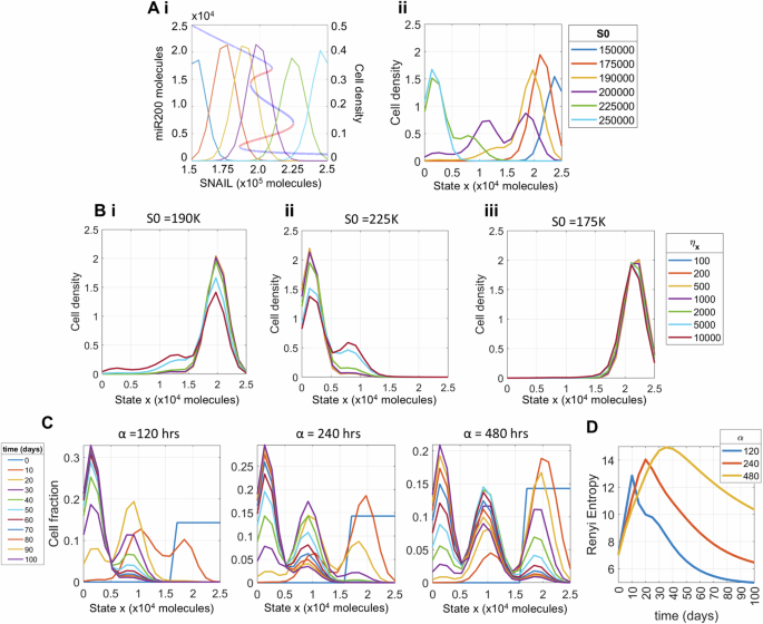
Empirically reduced single cell state variable x, showing that the reduced system captures the full EMT network dynamical response; and the combined influence of biochemical noise with input signal dynamical response in modulating the phenotypic heterogeneity of the cell population. Ai Bifurcation diagram showing stable (blue) and unstable (red) levels of miR-200 (y axis on left) for increasing SNAIL levels; and distribution of SNAIL levels among the cells (y axis on right) for different mean characteristics levels S0. Aii Distribution of cells along the state x of reduced EMT system for different distributions of SNAIL shown in (Ai) after a simulation time of 100 days starting from epithelial cells. B Changes in population’s phenotypic distribution with increasing levels of epigenetic noise ηx for SNAIL distributions with mean S0 = 190K (Bi) and 225K (Bii). For S0 = 175K (Biii), the population remains invariant to increasing noise. C Temporal changes in cell state distribution of the population for decreasing values of input signal SNAIL’s perturbation recovery rate (increasing values of the characteristic time ‘α’). D Time evolution of population’s heterogeneity (measured by differential entropy) for different α parameter values. Parameters used to generate plots, unless stated otherwise, are α = 120 h, ηx = 1000, ini pop Epi (see Fig. 4A, i), time = 100 days, S0 = 225K molecules, and division rate r is constant across phenotypes, given by r = 0.0182/h.
For example, with a SNAIL distribution of mean value (S0) of 200 K molecules, the bifurcation diagram depicts the possibility of the cell population to be distributed in all three states (Fig. 3Ai). We find that the asymptotic distribution of the state variable x from reduced system dynamics exhibits tri-modality, showing the co-existence of all three states, irrespective of the initial population condition (Fig. 3A, ii—initial population: all cells as epithelial, Fig. S2B—initial population: all cells as hybrid or mesenchymal). Similarly for a SNAIL distribution with mean S0 ∈ {190K, 225K, 150K, 250K} molecules, we observe respective combinations of phenotypes as in the bifurcation diagram of the full EMT network – co-existence of E and H (bimodal), co-existence of H and M (bimodal), epithelial (unimodal) and mesenchymal (unimodal) (Fig. 3A), thus providing further evidence of faithfully representing EMT dynamics through the sole variable x.
For multi-modal distributions of the state variable x, the exact phenotypic composition depends on relative stability of the multiple co-existing phenotypes. For example, we see a reduced share of H (intermediate x levels) cells for distribution of SNAIL levels that overlap significantly with those that have mean SNAIL levels corresponding to monostable E or monostable M regions (S0 = 190K, 225K molecules respectively), especially for a reduced standard deviation ηx of stochastic cell-state transition in state x (Fig. 3Bi, ii). Similarly, for distribution of SNAIL levels with mean S0 = 175 K molecules, although both E and M states co-exist (Fig. 3A, i), the relative stability of the E state is much greater than that of the M state, thus disallowing cells to make transition to the M state even at higher levels of ηx (Fig. 3B, iii).
As mentioned previously, the distribution of SNAIL levels and correspondingly that of the cell state x in a population can be attributed to stochasticity in biochemical reactions. Another type of perturbation in cellular variables (here, x and SNAIL) can arise when certain subpopulations are isolated and re-cultured independently. For instance, when the E, M and H prostate cancer subpopulations are segregated, they exhibit very different distributions after 2 weeks12. Similarly, the segregated EpCAM-high and EpCAM-low subpopulations in breast cancer have varied recovery dynamics45. Thus, in case of either internal (stochastic cell-state transition) or external (microenvironmental factors) perturbations, the rate at which the cellular variables recover towards the characteristic distribution can differ even though they eventually converge to the same equilibrium distribution. Thus, we next modulated the rate of recovery of SNAIL levels to mimic the scenario of extrinsic perturbation to the cell population by isolating distinct subpopulations and simulating (re-culturing) them independently.
The rate of recovery to perturbations in SNAIL levels is inversely correlated to the parameter α in our model, which captures the characteristic time of convergence of SNAIL levels to its equilibrium S043,46. For an extrinsic perturbation (e.g. enriched epithelial cells from a M cell majority population), we see that the time evolution of the population distribution slows down with increasing values of α (Fig. 3C). Furthermore, the slowed down dynamics increases cellular heterogeneity by causing the population to be distributed in all three states for a considerable interval of time, as quantified by differential entropy (Fig. 3D). In the example shown, population heterogeneity first increases as the population shifts from a majority of epithelial cells to being more uniformly distributed among the three phenotypes in the intermediate time points, and then decreases as the population becomes mainly composed of M cells. Similar observations can be made for other combinations of initial condition and mean S0 values of SNAIL distribution (Figs. S3, S4).
Overall, the interplay between deterministic and stochastic dynamics of cellular biomolecules shapes the population heterogeneity. This is done both by distributing cells in all plausible states permitted by the underlying regulatory network dynamics, and by slowing down the kinetics of cells towards equilibrium when perturbed by the external signal S.
Difference in phenotypic division rates reduces E-M heterogeneity, which could be recovered by increasing biochemical noise levels
We performed model simulations to see how an interplay between deterministic and stochastic effects on the cell state x, and input SNAIL, can impact the E-M heterogeneity patterns. So far, we considered all three phenotypic states (E, M and H) to divide at equal rates. To observe the additional influence of division rate differences on E-M heterogeneity we considered three possible scenarios—(a) case ‘r1’: all three phenotypes divide at the same rate, (b) case ‘r2’: both E and H cells divide at equal rates, while M cells divide at half the rate of E cells; and (c) case ‘r3’: both H and M divide at equal rates, which is half the rate of division of E cells. In practice, this means considering three different possible piecewise-constant functions r, as illustrated in Fig. 4A, ii. Across all these cases, the E state divides at either an equal or a faster rate than H and/or M cells. This constraint recapitulates the current experimental understanding that EMT may suppress cell cycle to varying extents, thus reducing the division rate of H and/or M cells35,47.
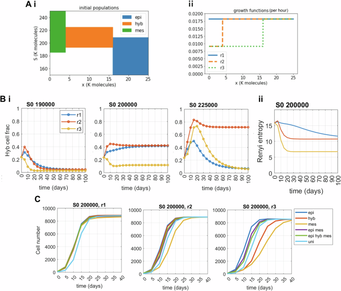
Ai Support of the different initial conditions: In each case, the initial condition is uniformly distributed on its support, and such that the total initial population equals 100 cells. Aii Profile of different growth functions, expressed per hour; ‘r1’: All three phenotypes divide at same rate; ‘r2’: E and H divide at equal rates, while M divide at half the rate of E cells; and ‘r3’: Both H and M divide at equal but half the rate of E cells. Bi Temporal changes in hybrid cell fraction in the population for different growth scenarios among phenotypes. Bii Time evolution of population’s heterogeneity (measured by differential entropy). C Population growth dynamics for different combinations of growth scenarios and initial condition; ‘epi hyb mes’ corresponds to an initial condition uniformly distributed on the three coloured domains of A1), and ‘uni’ to a uniform population on the whole rectangle [0, 25 K] × [150 K, 250 K]. For (B), the initial condition is uniformly distributed in all states. The input SNAIL mean (S0) levels used are mentioned for all the individual plots. Other parameters used to generate plots are α = 120 h, ηx = 1000, and the division rate (r) of the epithelial phenotype is 0.0182/h.
First, we investigated how the phenotypic composition of the population changes with different division rate scenarios (Fig. 4, Fig. S5). For uniformly distributed cells in all three E (epi), H (hyb), and M (mes) states (Fig. 4A, i) and SNAIL distribution with mean S0 = 190 K or 200 K molecules that predominantly enables an E state with/without H state, the reduced growth of M cells has very slight effects on phenotypic composition over the time course, as expected (Fig. 4B, i). The initial peak in hybrid cell fraction for the ‘r2’ growth scenario is the combined effect of M to H state transition and a relatively higher division rate of H cells. However, when H cells also have reduced proliferation (growth scenario ‘r3’), we see a lasting change in the phenotypic composition as E cells become dominant because of higher division frequency (Fig. 4B, i—S0 = 200K). For the input SNAIL distribution with a mean value S0 of 225 K molecules that majorly supports H and M phenotypes, in the case ‘r2’, the growth advantage provided to H cells enables their dominance in the population on the long run, when compared to the growth scenarios of ‘r1’ or ‘r3’ where both H and M cells proliferate at equal rates (Fig. 4Bi, S0 = 225K). The initial peaks in H fractions are combined effects of E to H transitions with either growth similarity or advantage of H cells over M cells.
The overall change in phenotypic composition can be calculated using differential entropy as a heterogeneity score (Fig. 4B, ii). Although growth scenarios ‘r1’ and ‘r2’ have the same phenotypic composition and an equal heterogeneity score eventually, the growth scenario ‘r1’ shows a much smoother change in heterogeneity values from the initial levels because of all three phenotypes being equally proliferative. Next, we looked at the effects of increasing level of epigenetic noise level ηx in cell state x on phenotypic composition laid down by division rate differences (Fig. S6A–D). For S0 = 190K and 200K, where the H state is less dominant than the E state (Fig. 4B), increasing the noise levels (from ηx = 1000 to ηx = 5000) in state x causes more cell-state transitions, raising the frequency of the H phenotype in population for all growth scenarios (Fig. S6B). However, as for S0 = 225K and growth scenario ‘r2’ where the hybrid phenotype is the dominant state, increasing the noise ηx level (from ηx = 1000 to ηx = 5000) raises M fractions in the population even though M cells are dividing slowly (Fig. 4B, i; Fig. S6B, C). Overall, we observe an increase in population heterogeneity with higher noise levels in state variable ‘x’, irrespective of the growth scenario (Fig. 4Bii, Fig. S6D).
After observing changes in phenotypic composition for different growth scenarios, we moved on to see how total cell population grows for combinations of initial conditions and growth scenarios. We considered six different conditions—isolated E, H, and M population, uniform mixture of either E and M or E, H and M cells, and uniform distribution of cells in all possible cell states x and input SNAIL levels.
When all the phenotypic states are dividing at equal rates, the total number of cells does not vary across different initial conditions. However, with M dividing slower than E and H cells (growth scenario ‘r2’), we see that an initially mesenchymal population has slower population growth compared to other initial conditions. Similarly, with both H and M cells dividing slower than E (growth scenario ‘r3’), initial conditions having component of either H or M cells divide slower than isolated (pure) E cells. Also, as transition from H to E is much more probable than M to E transitions, presence of hybrid cells in the population increases the overall division rate (Fig. 4C compare ‘hyb vs mes’, and ‘epi mes’ vs ‘epi hyb mes’ initial conditions for S0 = 200 K, ‘r3’ growth scenario). Further, increasing the level of cell transition stochasticity (from ηx = 1000 to ηx = 5000) causes more state transitions rendering lesser variability in the growth dynamics by quickly equalising the effect of differences in the initial conditions (Fig. S6E).
Addition of resource competition among subpopulations enables bistability in phenotypic composition and bi-phasic growth of total cell number
Although there was limitation to growth to the cell population so far via a logistic growth term, all subpopulations were considered to present equal resource competition to each other. More specifically, the death rate d(y)ρ(t) in Equation (5) is considered to be proportional to the total population size ρ(t), which supposes that all three subpopulations consume resources in the same amount. Here, we investigated how unequal resource competition among E, M and H affects the dynamic and asymptotic phenotypic composition of the cell population.
For this purpose, we developed a generalisation of Equation (5) with a more general growth term. For simplicity, we assumed that the SNAIL level is constant and equal to S0: = 200 K for all cells at all time. This generalised equation can then be written as
where
-
The advection function f is given by f(x) = fr(x, S0).
-
The ‘mutation’ function M is taken to be (M(x,z)=r(x)P(x-z){{mathbb{1}}}_{[0,25K]}(x)), with (P(x)=P(x):=frac{1}{{eta }_{x}}G(frac{x}{{eta }_{x}})), where G is the Gaussian function.
-
The death rate ρκ(t, x) is now computed as the integral of the cell density u(t, z) weighted by a kernel κ(x, z).
The choice of κ allows to include competition for resources which depends on the cells’ states. For instance, κ(x, z) > κ(z, x) models the fact that whenever cells with states x and z compete for resources, a cell with state z consumes more resources than a cell with state x. In the case where κ(x, z) = d(x), we recover equation (5), with ρκ(t, x) = d(x)ρ(t).
For simplicity, in the simulations of this section, we chose κ of the shape
where ({{mathbb{1}}}_{E}(x)=1) if x ∈ E = [16K, 25K] (epithelial cells) and 0 otherwise, ({{mathbb{1}}}_{H}(x)=1) if x ∈ H = [4K, 16K] and 0 otherwise, and ({{mathbb{1}}}_{M}(x)=1) if x ∈ M = [0, 4K] and 0 otherwise.
This choice of κ is to be linked with the Lotka-Volterra resource competition model: indeed, in the absence of state transition and advection, and by taking (r(x)={r}_{m}{{mathbb{1}}}_{M}(x)+{r}_{h}{{mathbb{1}}}_{H}(x)+{r}_{e}{{mathbb{1}}}_{E}(x)), one easily checks that the epithelial, hybrid and mesenchymal populations, given respectively by
satisfy the ODE model
In our simulations, we fixed r(x) = 0.0182 h−1 (corresponding to 38 h of doubling time), dm = dh = de = 1.82 × 10⁻⁷ /hr/cell (assuming per cell death is 104 times slower than birth), αmm = αhh = αee = αeh = αhe = 1, and we assumed that αme = αmh = : α and αem = αhm = : β. We ran simulations for different values of α and β, and different initial distributions. Here, the assumption is that E and H cells behave identically in terms of resource consumption and in how they compete with M cells.
We observe that for certain values of α and β, particularly α ≥ 1 and β > 1, the phenotypic composition of the population has two asymptotic states, which can be reached depending on the initial distribution of the population (Fig. 5A, Figs. S7Ai, S8, S9). For example, the initial population containing more than 30% of M cells converges to high M cells fraction/numbers in the population, otherwise the asymptotic population is found to be dominated by H cells. Further, the bistable phenotypic composition remains intact even if the rates of cell-state transition are significantly reduced to minimal levels (ηx = 1, Fig. S7Aii). The range of competition coefficients (α and β) for which we have bistability in phenotypic composition may change when either the relative stability of E, M and H cells or their cell-state transition rates are varied (Fig. S10).
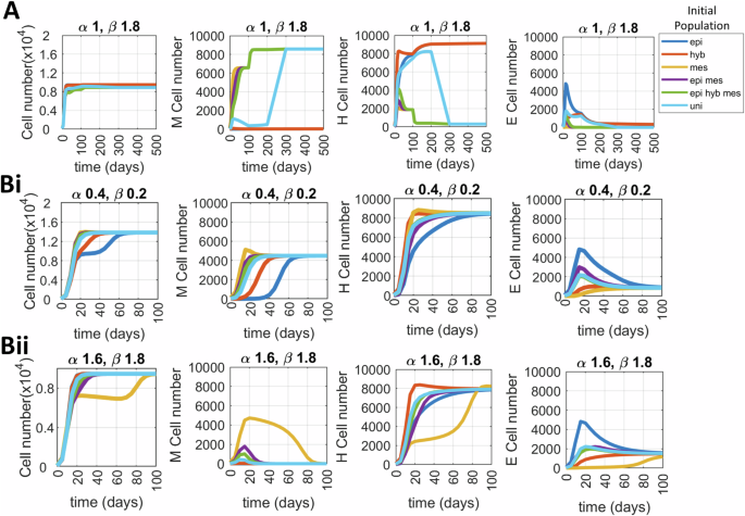
Model (12) is used to model resource competition between E, M and H cells. The self-interaction parameters of the resource competition for all three phenotypes are set to 1 and the E and H cells were assumed to be identical in terms of resource consumption. Therefore, their cross-interaction parameters is set to unity. Parameter α denotes resource competition from E and H to M cells and β denotes resource competition from M to E and H cells. A Two distinct steady-state phenotypic compositions of M and H hybrid arise when initial population contains low and moderate-to-high proportion of the M cells. Multi-stability in phenotypic composition occurs in small region of parameters α and β controlling resource competition (Figs. S8 and S9). B Biphasic growth pattern in total cell number. Biphasic growth is defined as presence of both quasi and asymptotic steady states at intermediate and long-term time instances, respectively. Bi the resource competition among E, M and H cells is small (both α and β < 1) and the initial cell population is E dominant (‘epi’ starting population), and Bii the resource competition among E, M and H cells is large (both α and β > 1) and the initial cell population is M dominant (‘mes’ starting population). The input SNAIL mean (S0) = 200 K, ηx = 2000, and the division rate (r) of the epithelial phenotype is 0.0182/h. Initial populations ‘epi’, ‘hyb’ and ‘mes’ correspond to 100 cells uniformly distributed on E, H and M respectively, ‘epi mes’ to a population of 50 cells on E and 50 cells on M, ‘epi hyb mes’ to a population of 33 cells on E, 33 cells on H and 33 cells on M, and uni to a population of 100 cells uniformly distributed on the whole [0, 25K] = E ∪ H ∪ M.
For certain initial population structures, we also observe biphasic growth in the total cell number, i.e. the presence of both quasi (apparent) as well as asymptotic steady states at the intermediate and long-term time instances, respectively (E ‘epi’ starting population in Fig. 5Bi and M ‘mes’ starting population in Fig. 5Bii). Since E and H cells present equal resource competition to each other, the total cells arising from starting E (epi) population saturates to the carrying capacity (10,000 cells) until the time population is devoid of M cells (40 days). Once M cells arise in the population due to phenotypic transitions, the total population gets boosted as the resource competition is low (α < 1 and β < 1). Thus, we see a biphasic growth pattern when starting with E population. Now, as the biphasic growth depends on the moment when the M cells arise in the population, reduced rate of cell-state transition (ηx = 1) further extends the duration of time spent in quasi steady state of low total cell counts (Fig. S7Bi). We also see biphasic response when there is high resource competition among E(or H) and M cells (α > 1 and β > 1) and M (‘mes’) starting population (Fig. 5Bii). Here, before the M cells reach the capacity of the population (10,000 cells), the high cell-state transition rates give rise to H cells within a short period of time, leading to significant resource competition and slowed down growth of both M and H cells. However, increasing population size of H cells and occurrence of E cells at later timepoints heavily lead to suppression of the M cells population by 80 days of simulation time. With reduced cell state transition, M cells gain dominance of the population before enough H cells appear in the population, and therefore, M cells suppress H and E cells number for all simulation time leading to loss of biphasic growth (Fig. S7Bii). When there is asymmetry in resource competition among E(or H) and M cells (α < 1 and β > 1 or α > 1 and β < 1), no significant patterns of bistability of phenotypic composition and biphasic total cell responses are seen (Figs. S8, S9 and S11).
Discussion
Several intracellular and intercellular regulatory and stochastic processes shape heterogeneity within a population. While several intracellular processes, such as non-linear transcriptional regulation, chromatin-based epigenetic regulation and microRNA-mRNA binding and complex degradation either individually or in combination can result into the existence of distinct gene expression states, the stochastic intracellular processes such as transcriptional bursting, asymmetric cell division, and cell-to-cell communication lead the cells to switch from one gene expression pattern to the other. Experimental data capturing temporal changes in population level heterogeneity while profiling cells for transcriptome and epigenome is only recent in the context of EMT. However, significant efforts have been made in multi-scale mathematical modelling of a cell population that is growing, dividing and changing its phenotypic distribution with intracellular state dynamics based on one or more regulatory processes. Here, we contribute to this rich multi-scale population modelling literature by developing a framework allowing us to study how E-M population heterogeneity is regulated by—(1) the regulatory and stochastic intracellular processes, (2) heterogeneity of growth rates, and (3) resource competition among distinct subpopulations.
Our analysis is based on a minimalistic three node EMT regulatory network with a characteristic phenotypic landscape (Fig. 2A)40. Our choice of a sufficiently simple network was based on the following criteria—(a) making the analysis computationally tractable, and (b) integrating multiple processes together—cell division, cell death, cell-state transition and intracellular regulatory dynamics. However, many more EMT regulatory networks with increasing complexity (nodes and types of interactions) have been identified over the past decade13,24. The identification and addition of new players that regulate EMT modify the relative stability of epithelial (E), hybrid (H) and mesenchymal (M) cell states, and thus, will change the phenotypic composition of the population at steady state for a given input signal and noise level in our study48,49,50. Nonetheless, the advection term in the developed PDE model can be easily updated with other regulatory networks to observe the resulting changes in the population composition.
We find that the existence of E-M heterogeneity in the cell population is a consequence of noisy biochemical process and constitutive signalling set at levels where the regulatory network operates in mono-stable or multi-stable regime (Fig. 3). Such necessity of both noise and multi-stability for getting a heterogeneous population may explain why certain breast cancer cell lines have homogeneous composition of E or M cells and others cell-lines are heterogeneous15,30. Further, the heterogeneity imparted by biochemical reaction noise gets suppressed because of growth rates differences among E-M subpopulations (Fig. 4B). On the other hand, lower biochemical noise can delay the rise in heterogeneity and growth of the total population if the phenotype composition of the population has a majority of slow growing cells to begin with (Fig. 4C)45. Such slow growth of cell population on reduced cell-state transitions may explain why stable mesenchymal cells are unable to form large tumours while plastic mesenchymal cells can in-vivo51.
The minimalistic EMT model considered here does not have a regulatory term for the input signal, so we assumed that the input has negative feedback onto itself and that its level in the population is distributed around the mean S0. The parameters α and S0 in input dynamics of S (Equation (11)) can be considered as the inverse of the birth rate and ratio of birth to death rates of S molecules, respectively. Therefore, the degradation and/or de-novo synthesis rates encoded in parameters α and S0 set the rate at which equilibrium phenotypic distribution is attained when individual subpopulations are isolated (Fig. 3). Such role of biomolecule turnover rates in cell-state switching has also been reported in other in-vitro and in-silico studies. For example, while cells possessing a transgene with long half-life of mRNA and protein were able to pass on the transgene expression through multiple cell divisions, the transgene expression in cells with short mRNA and protein half-life could not be transmitted for more than a few generations52. Similarly, an in-silico study showed how switch in the expression of a gene can be hindered by long half-life of its mRNA molecule53. In the context of E-M plasticity, it was observed that different sets of molecular markers take varying time to revert to the basal expression levels post EMT induction54. Thus, the timescales of spontaneous cell-state switching are determined by the molecular markers used to define the cell states.
By incorporating resource competition between E, H and M sub-populations, we either saw biphasic growth in total cell number or initial condition dependent asymptotic subpopulations levels (Fig. 5)55,56. Such density-dependent growth interactions have been thoroughly studied in the dynamics of sensitive and resistant cancer cells and used to retrospectively explain in vivo/clinical data. However, in addition to resource competition, various other factors, such as (1) juxtacrine and paracrine signalling among cancer cell subpopulations, and (2) interactions of tumour cells with extracellular matrix (ECM) and/or other stromal cells) can alter cell growth rates and influence overall population structure9,57. For example, cells that undergo EMT can secrete LOXL2 which increases collagen crosslinking in ECM, and ECM density and stiffness can induce EMT58. The developed Cell Population Balance model can be extended to capture the cellular interactions mentioned above and is considered the future directions of this study.
Mathematical models that capture dynamics of population-level heterogeneity resulting from regulatory and population dynamics of cells include Agent-Based models and Cell Population Balance models. Among the advantages of Agent-Based models are their ability to capture the evolution of heterogeneity with details at single cell levels. However, simulating Agent-Based models leads to prohibitive computational costs for a large number of cells. On the other hand, Cell Population Balance models capture the evolution of cell densities in a heterogeneous population, therefore inherently assuming a large population size. Further, the cell density computed in Cell Population Balance models can be directly mapped to output of flow cytometry experiments conducted at multiple timepoints for a population. Thus, over the past two decades, Cell Population Balance models have been used to combine complex regulatory phenomena, e.g. positive feedback loops59, caspase activation cascade during programmed cell death60, cell-to-cell communication61, and two mutually inhibiting nodes62, with stochastic processes like asymmetric cell division and stochastic biochemical reactions for phenotype-structured, and age-structured cell populations61,63,64
In our study, the simultaneous consideration of cell division, death, and state transition for the full EMT network lead to significant increase in the computational cost. Therefore, we reduced the existing model with two variables and one input signal to a model with a single variable and one input signal. The parameters of the reduced one-dimensional state derivative function (Fig. S2A) were set by minimising the error of its resulting dynamics with that of the full EMT model.
Our approximation and parameterisation of the state derivative function are in line with efforts over the last decade to use experimental flow cytometry and cell counts data to either parameterise the cell population balance model or optimally choose the functional form of state dynamics along with other parameters that fit the data well60,63,65. Notably, these studies use Maximum Likelihood approaches to parameterise the system since their aim is to fit data rather than approximate an already existing but more complex model.
To model stochasticity in the cell’s state resulting from, for example, transcriptional bursting or asymmetric cell division, we have generalised intracellular noise by considering a general transition kernel, which we then assumed to be normally distributed around the current cell state by focusing on the case where stochasticity is mediated by cell division. We note that some literature has shown the individual contribution of each of the stochastic cellular processes on cellular heterogeneity59,61,66, and the model framework developed here can be easily used to account for other stochastic factors.
Our framework allows for the addition of a diffusion term, as has also been done in the literature. Indeed, a second-order diffusion term is the PDE counterpart of adding a Brownian motion to the considered ODE as in ref. 43. The corresponding diffusion term can be recovered by a suitable scaling of our integral transition term as explained in ref. 67, which we have not done in the present work. Additionally, assuming the noise to be normally distributed gave us a handle on its extent (standard deviation), and therefore enabled us to comment on the changes in population heterogeneity with increasing levels of noise (Fig. 3B).
The main equation studied in this article (10) is in line with Cell Population Balance models usually employed for heterogeneous cell populations62,64,68,69. Nevertheless, we have chosen a rather common logistic shape for the growth term, which writes ‘(r(y) − d(y)ρ(t))u(t, y)’, with ρ(t) the total number of cells at time t, rather than a simple linear term as it is often done. From a biological point of view, this choice reflects the capacity for the cell population to self-regulate its growth due to density constraints. From the mathematical perspective, it guarantees that the size of the population does not blow up, i.e. remains bounded, and allows one to study how the population evolves in larger times.
Regarding the numerical implementation, we opted for a scheme from the family of particle methods: these schemes are indeed known to be well-suited in the context of PDEs with advection and ‘non-local’ terms, that is terms that involve the density of the cell population at all points. In our case, the selection term and the state transition term are both non-local terms, since the former depends on the population size ρ, and the latter is a convolution with the so-called ‘mutation function’ M.
Convergence of particle methods has been proved under conditions that are satisfied in our setting39. Compared with other methods used for the same type of problems, such as finite element methods70 or finite difference methods71, particle methods have several advantages. Firstly, they are easily adaptable upon modifying the model, which allows for greater flexibility in model design (in our case, useful when passing from the homogeneous description (6) to the full model with growth and cell-state transition (10), and then to the equation with generalised growth term (12)). Moreover, they are based on a Lagrangian description of the system, and do not require an underlying mesh. More precisely, the initial data is discretised by a set of points, whose positions in the state space are then made to evolve in time via the advection term: this allows to ‘follow’ the cell population as it converges towards regions of higher concentration. However, in the presence of state transition terms, particle methods are not asymptotic-preserving schemes39, which means that the particle approximation (15) does not correctly approach the solution of the PDE for very large times. To avoid this problem, we carry out the regulation process at each time step, as described in the ‘Methods’ Section.
Overall, we employed cell population balance modelling to analyse the combined effect of EMT regulatory dynamics with cell division and death, and stochastic cell state transition. The integration of these complex processes together was made possible thanks to an efficient PDE numerical integration scheme recently developed by some of us39.
Methods
Parameters for ODE (8) and (9)
We detail the parameters underlying ODE (8):
Functions ({H}_{Z,{mu }_{200}}), ({H}_{S,{mu }_{200}}), ({H}_{Z,{m}_{Z}}) and ({H}_{Z,{m}_{Z}}) are shifted Hill functions which write under the form
The associated parameters are given in Table 1.
The functions Yμ, Ym and L are defined by
where ({M}_{n}^{i}:=frac{{(mu /{mu }_{0})}^{i}}{{(1+mu /{mu }_{0})}^{n}}). Finally functions P and Q are given by
Parameters for these three functions are given in Table 2.
The additional parameters of ODE (9) are α = 0.15, and β(t) = 240 when S is non-decreasing, and β(t) = 720 when S is decreasing.
Reduction of the advection function
Let us introduce the segments, Iep = [150000, 185270.541082], Iep−mes = [185270.541082, 193286.5731462], Iep−hyb−mes = [193286.573146, 208817.635271], Ihyb−mes = [208817.635271, 224649.298597], and Imes = [224649.298597, 250000], which correspond respectively to the values of S for which the model is monostable (with a unique equilibrium point which corresponds to the epithelial phenotype), bistable (with two equilibrium points which correspond to the epithelial and the mesenchymal phenotypes), tristable, bistable (with two equilibrium points which correspond to the hybrid and the mesenchymal phenotypes), and monostable (with a unique equilibrium point which corresponds to the mensechymal phenotype), as can be seen on the bifurcation diagram (Fig. 2A).
The values of stable equilibrium points representing the three possible phenotypes slightly vary depending on the value of S as illustrated by the bifurcation diagram. We approximate each of them via a five-order polynomial interpolation, i.e. a polynomial of the form
Pmes(S), Phyb(S) and Pep(S) respectively approximate the mesenchymal, hybrid and epithelial phenotypes (three solid lines on the bifurcations diagrams), while Pu1(S) and Pu2(S) correspond to the unstable equilibrium points (two dotted lines in the bifurcation diagram). The coefficients defining these five polynomials are given in Table 3.
We can finally define our one-dimensional reduced function:
-
If S ∈ Iep: ({tilde{f}}_{r}(x,S)=-(x-{P}_{ep}(S))).
-
If S ∈ Iep−mes:
-
If x ≤ 0.5(Pmes(S) + Pu1(S)): ({tilde{f}}_{r}(x,S)=-(x-{P}_{mes}(S)))
-
If x ∈ [0.5(Pmes(S) + Pu1(S)), 0.5(Pu1(S) + Pep(S))], ({tilde{f}}_{r}(x,S)=x-{P}_{u1}(S))
-
If x ≥ 0.5(Pu1(S) + Pep(S)), ({tilde{f}}_{r}(x,S)=-(x-{P}_{ep}(S)))
-
-
If S ∈ Iep−hyb−mes:
-
If x ≤ 0.5(Pmes(S) + Pu1(S)), ({tilde{f}}_{r}(x,S)=-(x-{P}_{mes}(S)))
-
If x ∈ [0.5(Pmes(S) + Pu1(S)), 0.5(Pu1(S) + Phyb(S))], ({tilde{f}}_{r}(x,S)=(x-{P}_{u1}(S)))
-
If x ∈ [0.5(Pu1(S) + Phyb(S)), 0.5(Phyb(S) + Pu2(S))], ({tilde{f}}_{r}(x,S)=-(x-{P}_{hyb}(S)))
-
If x ∈ [0.5(Phyb(S) + Pu2(S)), 0.5(Pu2(S) + Pep(S))], ({tilde{f}}_{r}(x,S)=x-{P}_{u2}(S))
-
If x ≥ 0.5(Pu2(S) + Pep(S)), ({tilde{f}}_{r}(x,S)=-(x-{P}_{ep}(S)))
-
-
If S ∈ Ihyb−mes:
-
If x ≤ 0.5(Pmes(S) + Pu1(S)), fr(x, S) = −(x − Pmes(S))
-
If x ∈ [0.5(Pmes(S) + Pu1(S)), 0.5(Pu1(S) + Phyb(S))], ({tilde{f}}_{r}(x,S)=x-{P}_{u1}(S))
-
If x ≥, ({tilde{f}}_{r}(x,S)=-(x-{P}_{hyb}(S)))
-
-
If S ∈ Imes: ({tilde{f}}_{r}(x,S)=-(x-{P}_{mes}(S)))
We are looking for a function that can be written as a multiple of ({tilde{f}}_{r}), i.e.({f}_{r}=k{tilde{f}}_{r}), with k > 0. In order to choose the most suitable parameter, we look for the value of k that minimises the quantity
where for all x0 ∈ [0, 25K], S ∈ [150K, 250K], x(⋅ , S, x0) solves
and for all Z0 ∈ [0, 800K], (left(mu (cdot ,S,{x}_{0},{Z}_{0}),Z(cdot ,S,{x}_{0},{Z}_{0})right)) solves (8).
In practice, this integral has been approximated for T ∈ {10, 100, 1000} by the Riemann sum
with NS = Nx = NZ = 20, NT = 100, and for all i, j, k, l, ({t}_{i}=ifrac{T}{{N}_{T}}), ({S}_{j}=150K+jfrac{100K}{{N}_{S}}), (x{0}_{k}=kfrac{25K}{{N}_{x}}), and (Z{0}_{l}=lfrac{800K}{{N}_{Z}}), where x(⋅ , Sj, x0k) solves
(left(mu (cdot ,{S}_{j},x{0}_{k},Z{0}_{l}),Z(cdot ,{S}_{j},x{0}_{k},Z{0}_{l})right)) solves (8).
The value of the multiplicative constant which minimises (13) depends on T but we establish that, for T ∈ {10, 100, 1000} its value is rather insensitive to that of T: it is close to 0.02, which it the value that we select. The obtained function is shown in Fig. S2 for various values of S.
Numerical method
We start by normalising the model to work with the domain [0, 1] × [0, 1] rather than [0, 25K] × [150K, 250K]. By denoting A = 25K, B = 0, C = 100K, D = 150K, we check that for all t ≥ 0, (u(t,x,S)=frac{1}{AC}{u}_{re}(frac{x-B}{A},frac{S-D}{C})), where ure is the solution of
where for all (x,Sin {mathbb{R}}), ({f}_{re}(x,S):=(frac{1}{A}{f}_{r}(Ax+B,CS+D),frac{1}{C}{f}_{S}(CS+D))), rre(x, S): = r(Ax + B, CS + D), dre(x, S): = d(Ax + B, CS + D), ({M}_{re}(x,S,{x}^{{prime} },{S}^{{prime} }):=ACM(Ax+B,CS+D,A{x}^{{prime} }+B,C{S}^{{prime} }+D)), and ({u}_{re}^{0}(x,S):=AC{u}^{0}(Ax+B,CS+D)).
Thus, an approximation for ure provides an approximation for u. We make use of a particle method in order to approximate ure at different times (0 < T1 < . . . < TK, specified in each figure), applying the method introduced in ref. 39 to deal with a category of models to which (10) belongs. For a proof that the numerical scheme does successfully approximate the solutions of (10), we refer to ref. 39, while an introduction to particle methods can be found in ref. 38.
We choose an integer parameter N (N = 20 in our simulations), and we denote ({y}_{1}^{0},ldots ,{y}_{{N}^{2}}^{0}), the points of the grid of size N × N on [0, 1] × [0, 1]. For i ∈ {1, . . . , N2}, we solve the ODE
with initial conditions ({y}_{i}(0)={y}_{i}^{0}), ({w}_{i}(0)=frac{1}{{N}^{2}}) and ({v}_{i}(0)=frac{{u}_{re}^{0}({y}_{i}^{0})}{{N}^{2}}), on the first time interval ([0, T1]). The solution of this ODE is called Particle approximation of (10). To solve (15) on [0, T1], we use the Python function solve_ivp in module scipy.integrate, with the default solver which corresponds to an explicit Runge-Kutta method of order 572.
We then use a regularisation process, i.e. we compute the sum
with ({G}_{varepsilon }(x,S):=frac{1}{{varepsilon }^{2}}G(frac{x}{varepsilon })G(frac{S}{varepsilon })), with G the Gaussian function, and (varepsilon ={left(frac{1}{{N}^{2}}right)}^{gamma }), with γ ∈ (0.5, 1). In all our simulations, we choose γ = 0.8: this value has been chosen empirically by carrying out simulations in simple cases for which the behaviour of solutions is well known (for example in the absence of cell-state transition), and by comparing with other values of γ. The points ‘y’ at which we compute this sum are ({y}_{1}^{0},ldots ,{y}_{{N}^{2}}^{0}).
We repeat the process for each time interval, taking as initial data the approximation calculated at the previous time step (i.e. uN(Tk−1, ⋅)), to compute uN(Tk, ⋅).
We acknowledge that stochastic approaches might also be used to simulate such models.
Responses