Approaching maximum resolution in structured illumination microscopy via accurate noise modeling

Introduction
Fluorescence microscopy is a method of choice for studying biological processes in live cells with molecular specificity. However, the diffraction of light limits the experimentally achievable resolution for conventional microscopy to ≈200 nm1, setting a lower bound on the microscope’s ability to probe the molecular events underlying life’s processes. In response, there is a strong interest in developing experimental and computational superresolution methods that extend microscopy beyond the diffraction limit. Unfortunately, to date, most superresolution techniques strongly constrain the sample geometry, sample preparation, or data collection strategy, rendering superresolved live-cell imaging challenging or impossible. For example, stimulated emission depletion microscopy (STED)2 requires high laser power and point-scanning, although recent parallelized approaches have expanded its capabilities3. Localization-4,5,6,7 and fluctuation-based8,9 techniques require specific fluorophore photophysics and hundreds to thousands of images, limiting their applicability to live-cell imaging. Structured illumination microscopy (SIM)10,11 is an attractive alternative for superresolved live-cell imaging because it is compatible with standard sample preparation methods, requires only about ten raw images per frame, and uses lower illumination intensity leading to reduced phototoxicity and photobleaching.
In SIM, structured illumination of a sample, combined with incoherent imaging, translates high-frequency information from beyond the diffraction limit below the microscope band-pass, where it appears as moiré interference fringes. In linear SIM, this additional information is used in computationally reconstructing the underlying fluorescence intensity map with theoretically up to double the widefield resolution. By exploiting photophysics, non-linear SIM can achieve even larger resolution enhancements12,13. Many 2D SIM approaches use a set of nine sinusoidal illumination patterns, both rotated and phase-shifted, to generate near-isotropic lateral resolution improvement. However, other 2D patterns or random speckle patterns are also used for similar purposes14,15 often generated using gratings16 or spatial light modulators17,18.
The computational reconstruction framework used in recovering information beyond the microscope’s traditional spatial resolution limit often determines the effective resolution in SIM, due to the choices made in how to treat contrast degrading noise. Approaching the maximum recoverable resolution in the SIM reconstruction as warranted by the data, therefore, requires correctly treating the main sources of noise, Poissonian photon emission, and camera electronics19,20 by accurately modeling the physics of image formation.
Furthermore, the inherently stochastic nature of fluorescence imaging makes reconstructing the fluorescence intensity map, the product of the fluorophore density and the quantum yield, naturally ill-posed. Consequently, we must use a model that provides statistical estimates of the fluorescence intensity map from exposure-to-exposure fluctuations in photon counts. In the high SNR regime, where photon shot noise dominates camera noise, average photon counts allow accurate estimation of the noise statistics from the recorded pixel counts. The ill-posedness of a reconstruction is, therefore, less severe at high SNR.
However, fluorescence microscopy images often include low SNR regions due to low fluorophore density or low illumination power. Image-to-image fluctuations are large in such regions, and both photon shot noise and camera noise become important21, making it more challenging to estimate the fluorescence intensity map. For incoherent imaging methods such as SIM, the effective SNR also depends on the length scales of features present in the image. The SNR-spatial size relationship is naturally understood in the Fourier domain where short length scales correspond to high spatial frequencies. As a microscope’s incoherent optical transfer function (OTF) attenuates high spatial frequency information22, there is loss of contrast for small spatial features, regardless of the average photon count. The inherent loss of contrast worsens the ill-posedness of image reconstruction and makes it very challenging to distinguish small biological features from pixel-to-pixel variations in photon shots and camera noise. Put differently, the effective SNR in the recorded images decreases with increasing spatial frequency, making the high spatial frequency information especially susceptible to noise.
Image reconstruction challenges are further compounded in SIM where super-resolved fluorescence intensity maps are recovered by unmixing and appropriately recombining noisy, low-contrast information distributed through the collected raw images as shifting moiré fringes. However, image-to-image variation due to photon shot and camera noise at the single pixel level can produce intensity fluctuations indistinguishable from low-contrast fringes. Consequently, during the SIM reconstruction process, these noisy signals may masquerade as genuine moiré fringes, leading to high-frequency reconstruction artifacts such as hammerstroke23. Artifacts typically become particularly pronounced at low SNR and for moiré fringes near the diffraction cutoff frequency, where the OTF reduces the contrast as discussed earlier.
Multiple SIM reconstruction tools have been developed to limit artifacts in SIM reconstructions. The most common reconstruction algorithms24 rely on a Wiener filter to deconvolve and recombine raw images in the Fourier domain. However, these approaches may fail in low SNR regions and can introduce artifacts indistinguishable from real structures23,25 due to their sub-optimal treatment of noise. For instance, performing a true Wiener filter requires exact knowledge of the SNR as a function of spatial frequency. Unfortunately, it is difficult to estimate the exact relationship of SNR versus spatial frequency from the sample. Instead, approaches replace the true SNR with the ratio of the magnitude of the OTF and a tuneable Wiener parameter26. More sophisticated approaches attempt to estimate the SNR by assuming the sample signal strength obeys a power-law27, choosing frequency-dependent Wiener parameters based on noise propagation models28, or alternatively engineering the OTF to reduce common artifacts29.
The primary difficulty associated with these approaches, and what ultimately limits feature recovery near the maximum supported spatial frequency, is that the noise model is well understood in the spatial domain while SIM reconstructions are performed in the Fourier domain. Rigorously translating the noise model to the Fourier domain is challenging because local noise in the spatial domain becomes non-local in the Fourier domain and gets distributed across all spatial frequencies.
Many attempts at avoiding artifacts associated with Wiener filter-based approaches at low SNR24 have proven powerful. Yet they still treat noise heuristically and typically require expensive retraining or parameter tuning to reconstruct different biological structures or classes of samples such as mitochondrial networks30, nuclear pore complexes31, and ribosomes32. For example, one common strategy is to apply content-aware approaches relying on regularization to mitigate the ill-posedness of the reconstruction problem by e.g., smoothing the fluorescence intensity map or using prior knowledge of the continuity or sparsity of the biological structures. These approaches include TV-SIM33, MAP-SIM34, Hessian-SIM35,36, and proximal gradient techniques37,38,39.
Recently, many self-supervised techniques have been developed as well. One such technique uses implicit image priors such as deep image priors (DIP)40,41,42,43 and physics-informed neural networks (PINN)44,45,46, which are neural networks whose structure itself inherently constrains the output images. These self-supervised networks are typically optimized iteratively using the input raw images only but can have a tendency to overfit data without additional regularizers and may not be as accurate as fully supervised methods. On the other hand, recently developed deep-learning-based 2D-SIM approaches, including rDL-SIM47 and DFCAN/DFGAN48 train neural networks in a supervised fashion to recognize structures at the cost of requiring large datasets for training and have avoided out-of-focus background in 2D SIM data. While these methods are powerful, developing deep learning approaches that generalize to different SIM instruments and classes of samples remains an open challenge. Alternative approaches are therefore greatly needed that operate at low SNR and thus broadly apply to any mixed SNR sample type.
Here we present Bayesian structured illumination microscopy (B-SIM), a new SIM reconstruction approach capable of resolving features near the resolution limit warranted by data. B-SIM handles high and low SNR SIM data in a fully principled way without the need for assumptions about biological structures or labeled training data. Consequently, B-SIM simultaneously addresses many desiderata of SIM reconstruction approaches and offers a powerful general-purpose alternative to deep learning approaches. Specifically, B-SIM: (1) accurately models the stochastic nature of the image formation process; (2) permits only positive fluorescence intensities; (3) eliminates arbitrary constraints on the smoothness of biological features; and (4) is amenable to parallelized computation. These features are achieved by working in a parallelized Bayesian paradigm where every part of the image formation process, including Poissonian photon emission and camera noise, are naturally incorporated in a probabilistic manner and used to rigorously compute spatially heterogeneous uncertainty. Such a physically rigorous reconstruction method was previously inaccessible computationally.
This advancement in noise modeling results in contrast enhancement near the highest supported spatial frequencies permitting feature recovery in low SNR data at up to 25% shorter length scales than state-of-the-art unsupervised methods. Previous Bayesian approaches49 incorporated stochasticity but until now have not correctly incorporated physics due to their choice of Gaussian process priors that enforce spatial correlations on biological features, permit negative fluorescence intensity values, and do not apply at low SNR where the Gaussian approximation to the full noise model falters.
Results
B-SIM operates within the Bayesian paradigm where the main object of interest is the probability distribution over all fluorescence intensity maps ρ, termed posterior, as warranted by the data. The posterior is constructed from both the likelihood of the collected raw SIM images given the proposed fluorescence intensity map together with any known prior information such as the domain over which the fluorescence intensity map is defined via a prior probability distribution (see “Methods”). From the posterior probability distribution, we compute the mean fluorescence intensity map (leftlangle {boldsymbol{rho }}rightrangle) that best represents the biological sample. Furthermore, the posterior naturally provides uncertainty estimates for the fluorescence intensity maps, reflecting spatial variations in noise due to any heterogeneity.
As shown in Fig. 1, to learn the posterior over the fluorescence intensity maps, ρ, from which we compute the mean we first develop a fully stochastic image formation model taking into account photon shot noise and CMOS camera noise. This model allows us to formulate the probability of a candidate fluorescence intensity map given input raw images, a calibrated point-spread-function (PSF), illumination patterns, and camera calibration maps. As our posterior does not attain an analytically tractable form, we subsequently employ a requisite Markov Chain Monte Carlo (MCMC) scheme to draw samples from the posterior, and compute its mean and associated uncertainty mentioned earlier. Furthermore, we parallelize this sampling scheme by first noting that a fluorophore only affects a raw image in a small neighborhood surrounding itself owing to the PSF’s finite width. By dividing images into chunks and computing posterior probabilities locally, our parallelized approach avoids large, computationally expensive convolution integrals.

a SIM involves collecting fluorescence images (left) illuminated by structured intensity patterns (center). We utilize a point-spread function model (center)(PSF) and calibrate the camera noise parameters (right): gain (g), offset (o), and readout noise (σ). To infer the underlying fluorescence intensity map, we start from a small region (orange) and sweep over the entire sample in a parallelized fashion. b An image formation model, ({mathcal{M}}), involves the multiplication of an underlying fluorescence intensity map with illumination patterns and convolution with the PSF to obtain a noiseless image, μ, which is then corrupted by photon shot noise and camera noise. c A Monte Carlo algorithm to sample candidate fluorescence intensity maps from the posterior probability distribution. Based on the current sample (orange) we propose a new sample for the fluorescence intensity map (blue) and compute its corresponding posterior probability. Favoring higher probability, we stochastically accept or reject the proposed fluorescence intensity map and update the current fluorescence intensity map. We average many samples of fluorescence intensity maps after convergence to obtain B-SIM reconstruction (right). WF and B denote widefield image and B-SIM reconstruction, respectively.
To validate B-SIM, we reconstruct SIM data in a variety of scenarios briefly highlighted here, and demonstrate that B-SIM surpasses the performance of existing algorithms both at low SNR and, surprisingly, high SNR. First, as proof of concept, we consider simulated fluorescent line pairs with variable spacing generated from a known imaging model and demonstrate the best performance achievable under ideal conditions. Next, we consider an experimental test sample with variable-spaced line pairs. This demonstrates that B-SIM retains excellent performance under well-controlled experimental conditions. Finally, we analyze experimental images of fluorescently labeled mitochondria in live HeLa cells, where experimental imperfections in the illumination, out-of-focus background fluorescence, and pixel-to-pixel variation in camera noise introduce challenges in SIM reconstruction. We note here that while 9 raw images corresponding to 3 orientations and 3 phase shifts (per orientation) of the illumination patterns are the standard for SIM to isotropically recover super-resolved data in the Fourier domain, fewer raw images may be used. However, the quality of reconstruction would be sample-dependent. If the features to be recovered have a preferred direction, illumination patterns perpendicular to that direction may be used to recover the features without using images for other orientations. Because of this sample dependency and lack of generality, we did not focus on testing reconstruction quality against a number of raw images.
In each case, we compare B-SIM with reconstructions using Wiener-filter based methods, particularly HiFi-SIM29 implementation with the default choice of parameters, and optimization based approaches, including FISTA-SIM38,39. We find that B-SIM provides increased fidelity and contrast for short length scale features at both high and low SNR as compared to existing state-of-the-art approaches.
Extending beyond unsupervised approaches, we compared the performance of B-SIM to deep learning-based rDL-SIM47 pre-trained on publicly available TIRF-SIM microtubule data50 provided by the authors of47,48 themselves. For the comparison, we generated experimental TIRF-SIM microtubule data using similar experimental conditions as the training data including camera model, magnification, and numerical aperture. Following the procedure from ref. 47, we denoise the raw SIM images using the provided microtubule-specific neural network. After denosing, we reconstruct SIM images using Wiener-filter-based methods. We find that B-SIM produces improved contrast, as shown in Supplementary Fig. S11, and demonstrates the difficulty in the generalizability of the currently available supervised methods.
Simulated data: line pairs
To demonstrate B-SIM performance under well-controlled conditions, we simulated a fluorescence intensity map of variably spaced line pairs with separations varying from 0 to 330 nm in increments of 30 nm. The sample is illuminated by nine sinusoidal SIM patterns with a frequency 0.9 times that of the Abbe diffraction limit, assuming NA = 1.49 and emission light wavelength λ = 500 nm. With these microscope parameters, the maximum supported spatial frequency for widefield imaging is (2,{rm{NA}}/lambda approx {left(168,{rm{nm}}right)}^{-1}), while the maximum recoverable frequency in SIM is (3.8,{rm{NA}}/lambda approx {left(88,{rm{nm}}right)}^{-1}). We generated simulated datasets at both high SNR, where photon shot noise is the dominant noise source, and at low SNR, where both shot noise and camera noise are significant.
For the high SNR dataset, we generated raw SIM images with up to ≈1000 photons per pixel. In Fig. 2a, b, we show SIM reconstructions of the fluorescence intensity maps obtained using B-SIM and compare them with HiFi-SIM and FISTA-SIM. At high SNR, all three approaches produce high-quality fluorescence intensity maps with minimal artifacts. We find that, according to the Sparrow criterion, the widefield image resolves the 180 nm line pair, HiFi-SIM resolves the 120 nm line pair (see Supplementary Fig. S2 for reconstructions using different choices of HiFi-SIM parameters), and both FISTA-SIM and B-SIM resolve the 90 nm line pair, approaching the theoretical limit discussed above. To further assess the resolution and contrast enhancements obtained across various methods, we also plot the intensity along line cuts showing the line pairs separated by 90 nm and 120 nm. Here we clearly see that B-SIM produces significantly enhanced contrast for both line pairs, with over ≈40% intensity drop in the center for the 90 nm line pair as compared to ≈5% drop in the FISTA-SIM reconstruction. Indeed, in comparison with HiFi-SIM, B-SIM recovers significantly higher contrast for line pairs with separations <150 nm. We attribute the enhanced contrast obtained by B-SIM to its physically principled incorporation of noise as compared to other approaches.
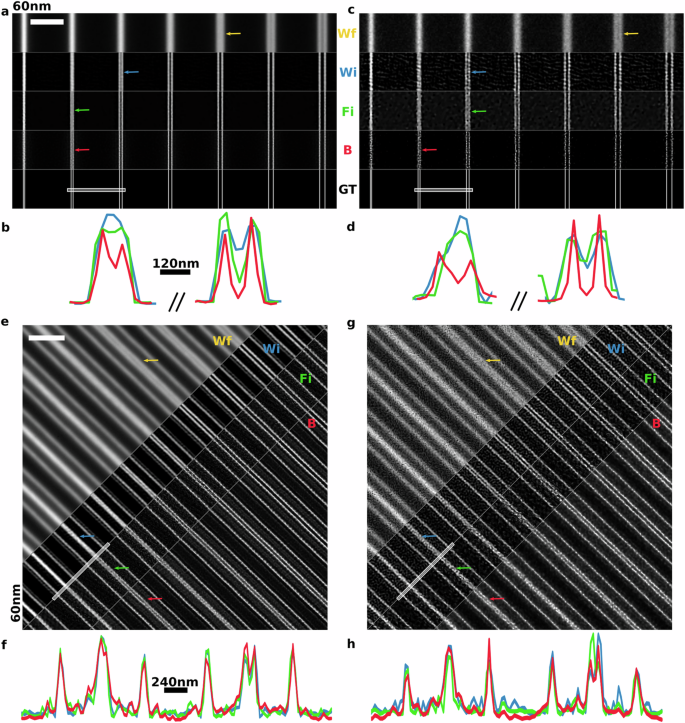
a Simulated line pairs with spacing ranging from 60 to 240 nm in steps of 30 nm at high SNR. We show the pseudo-widefield (Wf) image obtained by averaging raw data, and ground truth (GT) image, together with SIM reconstructions using Wiener filter (Wi), FISTA-SIM (Fi), and B-SIM (B). Scale bar 1.5 μm. Colored arrows indicate the line pair resolved according to the Sparrow criterion. b Line cuts corresponding to the white line in (a). All reconstruction methods resolve the 120 nm-spaced line pair. Both FISTA-SIM and B-SIM resolve the 90 nm-spaced line pair, but B-SIM does so with higher contrast. c Simulated line pairs as in (a), but at low SNR. d Line cuts corresponding to (c). All reconstruction methods resolve the 120 nm line pair, but only B-SIM resolves the 90 nm line pair. e Experimental images and reconstructions of variably spaced line pairs on an Argo-SIM calibration sample at high SNR. Line pairs have spacings of 60–330 nm in 30 nm steps. Scale bar 2.0 μm. f Line cuts corresponding to (e). All methods resolve the 120 nm-spaced line pair (right) with similar contrast, and no methods resolve the 90 nm line pair (left). g Experimental images as in (e), but at low SNR. Wiener and FISTA-SIM introduce reconstruction artifacts. h Line cuts corresponding to (h). Only B-SIM resolves the 120 nm spaced line pair.
We also tested B-SIM’s robustness against errors in illumination patterns for the high SNR dataset. By adding erroneous shifts to the phases of the sinusoidal patterns used to compute the posterior, we find that the reconstruction is robust for phase errors up to order 20°. Significant artifacts appear in the reconstruction for larger errors, as shown in Supplementary Fig. S1.
Next, we consider a more challenging low SNR simulated dataset with up to ≈40 photons per pixel in each raw SIM image, Fig. 2c, d. At this signal level, photon noise results in larger exposure-to-exposure variance, and camera noise becomes significant. Furthermore, a simple Poissonian or Gaussian approximation of the noise model is not enough for a high-fidelity reconstruction. Due to the decreasing effective SNR with increasing spatial frequency, we expect the achievable contrast at shorter length scales to be lower than that of the high SNR case. This intuition is confirmed in Fig. 2, where we find that widefield only resolves the 210 nm line pair, instead of the 180 nm as in the high SNR case. At low SNR, SIM reconstruction becomes increasingly challenging as evidenced by increasing hammerstroke artifacts visible in the HiFi- and FISTA-SIM reconstructions. Here, both HiFi-SIM and FISTA-SIM are unable to resolve separations below 120 nm. However, we find that B-SIM still resolves the 90 nm line pair without hammerstroke artifacts.
To quantitatively compare the various reconstruction methods, we also calculated the mean-square error (MSE) and peak signal-to-noise ratio (PSNR) using the known ground truth image, as shown in Supplementary Table S1. For the high SNR data, we find that both B-SIM and FISTA-SIM more faithfully reconstruct the line pairs than the other methods, and achieve similar scores. More critically, for the low SNR data, B-SIM achieves the highest scores. To further improve the smoothness in the B-SIM results shown in Fig. 2a–d, it is possible to generate more MCMC samples, albeit at a higher computational cost.
Experimental data: Argo-SIM line pairs
Having demonstrated significant contrast improvement by B-SIM on simulated data near the maximum achievable SIM resolution, we next recover fluorescence intensity maps from experimental images of variably spaced line pairs on an Argo-SIM calibration slide. The line pairs are separated by distances varying from 0 nm to 390 nm in increments of 30 nm. We illuminated these line pairs with nine sinusoidal illumination patterns with three orientations, each with three associated phase offsets and a pattern frequency of ≈0.8 times that of the Abbe diffraction limit. The peak emission wavelength for this sample was λ = 510 nm, and the objective lens had NA = 1.3. Here, the diffraction-limited resolution is ≈196 nm, and the achievable SIM resolution is ≈109 nm. With these parameters, we generated two datasets, one at high SNR, and one at low SNR per exposure.
Unlike in analyzing simulated line pairs where the illumination pattern is specified by hand, in working with Argo-SIM slides, we must estimate the illumination patterns from the raw fluorescence images as a pre-calibration step prior to learning the fluorescence intensity map. We estimate pattern frequencies, phases, modulation depths, and amplitudes from high SNR images using Fourier domain methods18, and generate one set of illumination patterns to be used for Wiener, FISTA-SIM, and B-SIM reconstructions. An independent approach for pattern estimation might not be feasible in all experimental circumstances. Joint pattern and fluorescence intensity map optimization is an interesting potential extension of B-SIM. We do not pursue this further in this work due to the increase in computational expense entailed in this joint inference.
For the high SNR dataset, we generated raw SIM images with up to ≈200 photons per pixel, Fig. 2e, f. Here, all SIM reconstruction methods generate high-quality fluorescence intensity maps with minimal artifacts. HiFi-, FISTA-, and Bayesian-SIM reconstructions all resolve the 120 nm line pair, with B-SIM resulting in the best contrast. Unlike for the simulated sample, none of the line pair spacings here are right at the diffraction limit, explaining why B-SIM does not resolve an extra line pair compared with other methods here. We also note some ringing in the reconstructions around line pairs, which we suspect is a side-lobe artifact. These artifacts typically appear in sparse samples where bright sources of light pollute dim neighborhoods, resulting in extra background noise that can overwhelm weak signals in those pixels. This background in combination with Fourier transforms being performed on small grids for convolutions, results in oscillations appearing around the main signal peaks.
For the low SNR dataset, we generated raw SIM images with up to ≈40 photons per pixel by using a shorter illumination time. We found that HiFi-SIM was not able to accurately estimate the illumination pattern parameters from this low SNR data, resulting in artifacts as shown in Supplementary Fig. S3, so instead, we used our mcSIM Wiener reconstruction18. As for the simulated data, Wiener-, and FISTA-SIM amplify high-frequency noise leading to significant reconstruction artifacts and these methods no longer clearly resolve the 120 nm line pair with high contrast, as shown in Fig. 2g, h. On the other hand, B-SIM introduces fewer high-frequency artifacts and continues to resolve the 120 nm line pair.
Experimental data: mitochondria network in HeLa cells
Next, we consider B-SIM’s performance on experimental images of dynamic mitochondrial networks in HeLa cells undergoing constant rearrangement in structure through fission and fusion with formations such as loops30,51,52. We perform live cell imaging to avoid mitochondria fixation artifacts53 using the same experimental setup as for the Argo-SIM sample. However, now we collect two sets of images—one with an emission peak of 569 nm to observe evolving mitochondrial cristae and a second with an emission peak of 660 nm to demonstrate the possibility of higher contrast reconstructions while reducing background and photodamage. We also adjust the absolute SIM pattern frequency to remain fixed at ≈0.8 the diffraction limit. As in the previous cases, we collect datasets at different SNR. In these datasets, due to high variation in fluorophore density along the mitochondrial network, the photon emission rate or SNR varies significantly throughout an image, posing a challenge for existing SIM reconstruction algorithms.
In Fig. 3, we show reconstructions of mitochondria cristae labeled with PKmito RED fluorophores. We collected three sets of SIM images by decreasing the illumination intensity by a factor of 10 each time, starting from the high SNR images with an average photon count of approximately 762. All of the three reconstruction methods resolve cristae for the high SNR SIM images, however, B-SIM clearly produces higher contrast with ≈50% more dip in intensity in the gaps between cristae compared to both FISTA- and HiFi-SIM, as shown with line cuts. As the camera noise increases relative to photo counts, we see FISTA-SIM amplifying noise and is not able to distinctly resolve cristae from both intermediate- and low SNR images; see Supplementary Fig. S5 for FISTA-SIM reconstructions using different choices of regularization parameter. While HiFi-SIM is able to resolve some cristae at intermediate SNR (see Supplementary Fig. S4 for HiFi-SIM reconstructions using different parameter choices), B-SIM, in a similar fashion to the high SNR case, again provides significantly higher contrast. Furthermore, B-SIM is able to distinctly resolve some cristae gaps that HiFi-SIM is unable to, as shown with line cuts. For the low SNR images, the MATLAB version of HiFi-SIM is unable to estimate patterns correctly, as shown in Supplementary Fig. S6, resulting in an unusable reconstruction. We, therefore, use the standard Wiener-SIM implementation18 which, like FISTA-SIM, significantly amplifies noise. B-SIM on the other hand does not show any noise amplification and show cristae structures, however, dominant camera noise causes significant loss of information resulting in small deterioration of reconstruction quality as compared to higher SNR images.
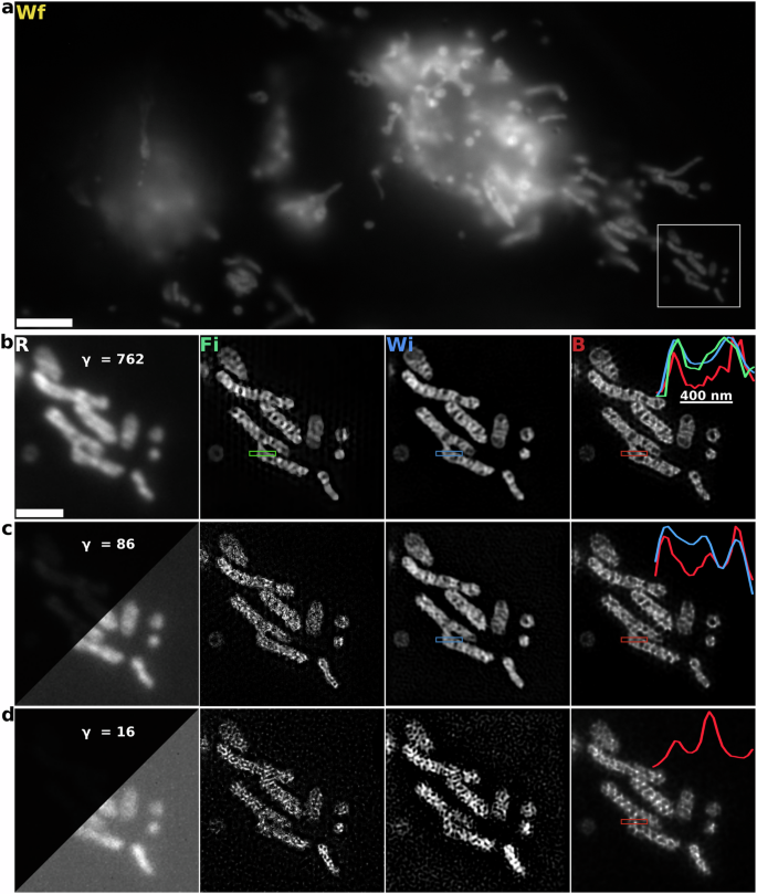
a 1024 × 454 pseudo-widefield (Wf) image of the mitochondria network in HeLa cells labeled with PKmito RED dye. Scale bar 5 μm. b SIM raw image (R) and reconstructions using Wiener filter (Wi), FISTA-SIM (Fi), and B-SIM (B) methods. γ parameter shows the average photon count in the image. Scale bar 2 μm. Line cuts from the three reconstructions are compared in the rightmost panel. c Same as in b at intermediate SNR. In the raw image, the left triangular half shows an image with the same color scaling as in (b). The right half rescales the image for visual convenience. We do not show line cuts for the FISTA-SIM reconstruction as it has significantly deteriorated. d Same as in c but at very low SNR. We do not compare line cuts as both FISTA- and Wiener-SIM reconstructions have significant noise amplification. The three sets of raw images at different SNR were taken at approximately 1.2 s intervals.
Unlike for the variably-spaced line pairs, there are no features in the mitochondrial network of known size we can use to directly infer the resolution achieved by the various SIM reconstruction methods. To obtain a quantitative estimate, we rely on image decorrelation analysis54. We estimate the achieved widefield resolution to be 260 nm compared with 150 nm for the Wiener reconstruction, and 94 nm for B-SIM, indicating improvement which broadly agrees with our observations in Fig. 3b, c. Lastly, we do not report results for FISTA-SIM as the decorrelation analysis relies on phase correlations in the Fourier domain that are strongly affected by the total variation (TV) regularization.
We note that decorrelation analysis provides a resolution estimate of 94 nm, smaller than the Abbe limit of 121 nm. However, this does not mean that B-SIM achieves resolutions better than the Abbe limit. Because decorrelation analysis relies on phase correlations present in the raw data in Fourier space, it likely indicates that B-SIM effectively smooths the reconstruction on spatial scales of the order of, and slightly smaller than, the diffraction limit. On the other hand, decorrelation analysis relies on identifying the maxima in correlation-versus-resolution curves for a sequence of high- and low-pass filters.
Now, while mitochondria are commonly imaged using fluorescent labels that emit near 500 nm wavelength to gain resolution55, the use of far-red fluorescent labels makes the data presented here particularly challenging for recovering small features in mitochondria networks. On the other hand, improvement in SIM reconstructions using such labels could be significantly advantageous because longer excitation wavelengths can reduce phototoxicity, background fluorescence, Rayleigh scattering, and Raman scattering56. Reduction in background at longer wavelengths is clearly visible in the interior of the cells in the widefield image in Fig. 4 as compared with shorter wavelength images in Fig. 3.
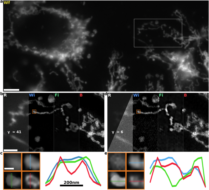
a 1024 × 454 pseudo-widefield (Wf) image of the mitochondria network labeled with MitoTracker Deep Red dye. Scale bar 5 μm. b We compare raw image (R), Wiener filter (Wi), FISTA-SIM (Fi), and B-SIM (B) reconstruction methods for the inset in (a). At high SNR, all methods capture superresolution information with limited reconstruction artifacts. γ parameter shows the average photon count in the image. Scale bar 2.0 μm. c Region of interest corresponding to the orange box in b shown in widefield (upper-left), Wiener, FISTA-SIM, and B-SIM. Scale bar 300 nm. Line cuts (right) demonstrate that B-SIM recovers more superresolution information than other methods without noise amplification. d Low-SNR SIM reconstruction of the same sample using a shorter illumination time. This image is acquired a few seconds after the images in (b). In the raw image, the left triangular half shows an image with the same color scaling as in (b). The right half rescales the image for visual convenience. e Region of interest from the inset in (d). Small shifts in the loop shown in the inset result from the continuously evolving mitochondria network.
For the high SNR longer wavelength dataset, we generated raw SIM images with on average ≈41 photons-per-pixel, Fig. 4b. Here, as before, HiFi- and FISTA-SIM produce reasonable reconstructions showing high-resolution features. FISTA-SIM introduces reasonably strong staircase artifacts57. On the other hand, B-SIM achieves significantly better contrast at short-length scales, more clearly revealing mitochondrial morphology. To illustrate the differences in these reconstructions, we focus on a tubular loop approximately 195 nm in diameter (Fig. 4c) and display a line cut. HiFi-SIM, on the other hand, is unable to resolve the central dip in fluorescence within the loop. We note here that since we have chosen a relatively background-free region of interest, honeycomb artifacts should be minimal and the loop is mostly likely real. Furthermore, we estimate the achieved widefield resolution to be 325 nm compared with 180 nm for the Wiener reconstruction, and 131 nm for B-SIM, indicating ≈25% improvement which broadly agrees with our observations in Fig. 4b, c.
Lastly, for the low SNR dataset, we generated raw SIM images with on average ≈6 photons per pixel, Fig. 4d. These images were taken approximately one second later to the high SNR images, and so we expect the morphology to remain the same. The HiFi-SIM reconstruction shows high-frequency noise amplification artifacts. These are avoided in the FISTA-SIM by applying a strong regularizer, which, however, significantly reduces the achievable resolution. On the other hand, B-SIM results in high-resolution reconstruction. We consider the same mitochondrial loop structure as before and find that it is resolved in both HiFi- and B-SIM. Applying decorrelation analysis, we find similar results as before where the widefield resolution is 430 nm, compared with 176 nm for the Wiener reconstruction and 131 nm for B-SIM.
Uncertainty in B-SIM reconstruction and statistical estimators
Bayesian inference using MCMC sampling techniques to draw samples of candidate fluorescence intensity maps from a posterior naturally facilitates uncertainty quantification over fluorescence intensity maps. Each MCMC sample generated by B-SIM represents a candidate fluorescence intensity map. An appropriate statistical estimator, the mean in this paper, provides the final representation of the fluorescence intensity map, and the extent of sample-to-sample variation provides a measure of confidence in that map.
In Fig. 5a–d, we show reconstructions performed on high SNR simulated line pairs and experimental HeLa cell images of the previous sections along with line cuts of mean fluorescence intensity map and 50% confidence intervals computed from posterior probability distributions shown as heatmaps. We confirm the existence of features that appear in B-SIM reconstructions in the previous sections based on very low absolute uncertainties where intensity dips occur between line pairs and in the center of loop-like structures in the mitochondria network. In the supplementary Fig. S7, we show the posterior distributions with confidence intervals for the low SNR reconstructions of the previous sections, as well as how to use MCMC samples collected by B-SIM to generate a visual representation of a posterior probability distribution.
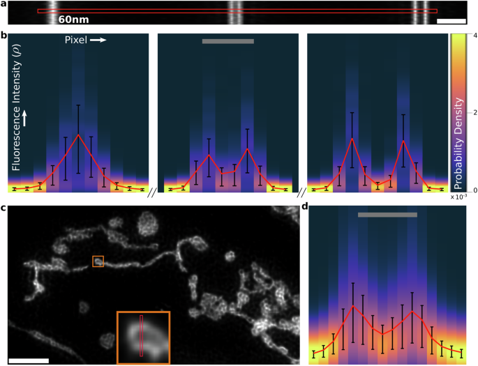
a B-SIM reconstruction for the high SNR simulated line pairs of Section “Simulated data: line pairs”. Scale bar 300 nm. b Marginal posterior probability distributions for fluorescence intensity at each pixel along the line cut in (a). The mean is shown in red, along with 50% confidence intervals in black. Scale bar 120 nm. c B-SIM reconstruction of mitochondria networks with high photon counts from Section “Experimental data: mitochondria network in HeLa cells”. Scale bar 2.0 μm. The region of interest (ROI) in the orange box is shown in the inset. d Marginal posterior distributions along the line cut in c. Same color map as in (b). Scale bar 195 nm.
In the B-SIM reconstructions presented in this paper, our preference for mean as the estimator is motivated by computational convenience. We find it easier to parallelize the process of generating MCMC samples by placing no expectation that fluorescence intensity maps be smooth, a priori. However, due to the ill-posedness arising from diffraction and noise, the lack of smoothness constraints results in most MCMC samples predicting pointillistic fluorescence intensity maps as they far outnumber probable smooth maps. With such a large degeneracy in the posterior distribution, recovering the most probable sample representing the true (smooth) fluorescence intensity map is a computationally prohibitive task. An efficient alternative is to use an integrative statistical estimator like the mean to recover pixel-to-pixel correlations in biological features warranted by the collected data. Supplementary Fig. S8 shows how the smoothness of the fluorescence intensity map for high SNR simulated line pairs of Section “Simulated data: line pairs” improves as the number of MCMC samples used to compute the mean is increased.
Additionally, in Fig. S8, we show maps of the inverse of the posterior coefficient of variation (CV), computed as the posterior mean to standard deviation ratio. In the same spirit as SNR for the Poisson distribution, inverse CV can be used to compare reconstruction quality in different regions of the image and is indicative of the effective SNR we discussed in the introduction resulting from diffraction or the OTF attenuating high-frequency information, making SIM reconstruction increasingly ill-posed. Indeed, in the case of simulated line pairs, the inverse CV decreases with separation as shown in Fig. S7. This increase in uncertainty in fluorescence intensity maps results from the increased model uncertainty where numerous candidate fluorescence intensity maps predict raw images nearly identical to the ones produced by the ground truth with similar probabilities. In fact, out of the approximately 400 samples or candidate fluorescence intensity maps collected by B-SIM for the line pairs, the similarity in morphology to the ground truth decreases with separation. While over 50% of the samples have two peaks for the 120 nm separated line pair, a large number of samples predict a merging of the two lines for the unresolvable 60 nm separated line pair and only about 15% of the samples have two peaks.
Discussion
We have developed a physically accurate framework, B-SIM, to recover super-resolved fluorescence intensity maps with maximum recoverable resolution from SIM data within the Bayesian paradigm. We achieved this by incorporating the physics of photon shot noise and camera noise into our model, facilitating statistically accurate estimation of the underlying fluorescence intensity map at both high and low SNR. Our method standardizes the image processing workflow and eliminates the need for choosing different tools or ad hoc tuning reconstruction hyperparameters for different SNR regimes or fluorescence intensity maps. We benchmarked B-SIM on both simulated and experimental data, and demonstrated improvement in contrast and feature recovery in both high and low SNR regimes at up to ≈25% shorter length scales compared with conventional methods. We found that B-SIM continues to recover superresolved fluorescence intensity maps with minimal noise amplification at low SNR, where Fourier methods are dominated by artifacts. Furthermore, because our Bayesian approach recovers a probability distribution rather than a single fluorescence intensity map, we used it to provide absolute uncertainty estimates on the recovered fluorescence intensity maps in the form of posterior variance and inverse CV to compare the quality of reconstruction in different regions. Lastly, we found B-SIM to be robust against phase errors in pattern estimates.
The generality afforded by our method comes at a computational cost that we mitigate through parallelization. If implemented naively, image reconstruction requires the computation of convolutions of the fluorescence intensity map with the PSF every time we sample the fluorescence intensity map from our posterior. This computation scales as the number of pixels cubed. However, the parallelization of the sampling scheme, as we have devised here based on the finite PSF size, reduces real time cost by a factor of the number of cores being used itself, moderated by hardware-dependent parallelization overhead expense.
Moving forward, we can extend and further improve our method in a number of ways. One improvement would be a GPU implementation where parallelization over hundreds of cores may significantly reduce computation time. Furthermore, more efficient MCMC sampling schemes, such as Hamiltonian Monte Carlo58,59, and more informative prior distributions over fluorescence intensity maps may be formulated to reduce the number of MCMC iterations needed to generate a large number of uncorrelated MCMC samples, accelerating convergence to a high-fidelity mean fluorescence intensity map.
Additionally, the sampling method developed here is generalizable and applicable to significantly improve other computational imaging techniques where the likelihood calculation is dominated by convolution with a PSF. As this describes most microscopy techniques, we anticipate our approach will be broadly useful to the imaging community, particularly dealing with modalities that are often SNR-limited, such as Raman imaging60,61. Alternatively, our approach could be applied to fully-principled image deconvolution and restoration.
In the context of SIM, our method’s extensions to other common experimental settings are also possible. For example, other camera architectures, such as EMCCD, requiring alternative noise models19 are easily incorporated into our framework. B-SIM’s versatility is also extendable by incorporating a more realistic PSF obtained by calibration measurements, learned from the samples directly, or simulated using a vectorial model to account for refractive index mismatch. One straightforward extension is 3D-SIM, where a modification of B-SIM would need to consider 3D-SIM patterns and 3D PSFs allowing for 3D-SIM reconstruction as shown in Sec. 3D-SIM and Supplementary Fig. S12.
Due to its generality and superior performance at both high and low SNR, we expect B-SIM to be adopted as a tool for high-quality SIM reconstruction. Furthermore, in the low-noise regime, fully unsupervised B-SIM is competitive with deep learning approaches. However, due to the use of a physics-based model, B-SIM is applicable to arbitrary fluorescent sample structures with no need to tune model parameters or retrain when switching from one class of samples to another, for instance, from mitochondria networks to microtubules.
Methods
Here we first setup an image formation model to generate noisy diffraction limited raw images for SIM where a sample is illuminated using multiple patterns, and then design an inverse strategy to estimate the fluorescence intensity map ρ(r) in the sample plane. In other words, our goal is to learn the probability distribution over fluorescence intensity maps given the collected raw images and pre-calibrated illumination patterns.
We use Bayesian inference, where a probability distribution over fluorescence intensity maps based on the predefined domain called prior is updated through a likelihood function that incorporates the experimental data/images.
Image formation model
Let ρ(r) be the fluorescence intensity at each point of space in the sample under a microscope. In SIM, we illuminate the sample a total of L times, with running index l, with sinusoidal spatial patterns given by
where A is the amplitude, ml is the modulation depth, kl is the frequency, and θl is the phase of the lth illumination pattern. This illumination causes the sample at each point in space to fluoresce with brightness proportional to its fluorescence intensity multiplied by the illumination at that point. The light from the sample passes through the microscope, and this process is modeled as convolution with the point spread function (PSF) of the microscope, which in this work, we assume to be an Airy-Disk22 given by
where f = 1/(2NA) is the f-number, λ is the emission wavelength, and NA is the numerical aperture of the objective lens. A more general PSF is also easily incorporated into our current framework.
The mean number of photons detected by the camera for the lth illumination pattern, μl, is the integral of the irradiance over the area of the nth pixel, An, plus a background, μb, that is unmodulated by the illumination pattern
which we write more compactly as
Here μl is the collection of expected brightness values on the camera for the lth illumination pattern and ⊗ is the convolution operation.
The number of photons detected on each pixel is Poisson-distributed
Finally, the camera electronics read out the pixel value and convert the measurement to analog-to-digital units (ADU). The number of ADU are related to the photon number by a gain factor, Gn, and an offset on. We model the effect of readout noise as zero mean Gaussian noise with variance ({sigma }_{n}^{2}). The final readout of the nth pixel, ({w}_{n}^{l}), is thus
With this observation model for each pixel, we can write the likelihood for a set of observations (raw images) as the product over probabilities of individual raw images given the fluorescence intensity map and camera parameters as
where w is the collection of readout values on the camera, ϕ is the collection of photon counts detected by the camera, C is the collection of all the camera parameters including the gain factor, offset, and readout noise variance for each pixel, and the vertical bar “∣” denotes dependency on variables appearing on the bar’s right-hand side.
Now, since the number of photons detected on the camera ϕ are typically unknown, we must marginalize (sum) over these random variables yielding the following likelihood
where, in the third line, we have used the chain rule for probabilities and ignored any dependency of photon detections on the camera parameters in the second term. Next, we note that expected values μl for Poisson distributed photon detections are deterministically given by the convolution in Eq. (4). This constraint allows us to write down the final likelihood expression as
where, assuming each camera pixel to be stochastically independent, we multiply the individual probabilities for camera readout on each pixel. We also note that we have not yet chosen a grid in the sample plane on which to discretize the fluorescence intensity map ρ(r). Such a grid is chosen according to convenience due to the simple additive property of the Poisson distributions that dictate the photons entering a camera pixel. For demonstration purposes, we assume that the fluorescence intensity map is Nyquist sampled on a grid twice as fine as the camera pixel grid. We denote this fluorescence intensity map on the mth point on this grid with ρm and the collection of these values with ρ.
Now, with the likelihood at hand, we move on to the formulation of an inverse strategy to estimate the fluorescence intensity map ρ.
Inverse strategy
Using Bayes’ theorem, we now construct the posterior distribution over the fluorescence intensity map and the unmodulated background ({mathcal{P}}left({boldsymbol{rho }},{{boldsymbol{mu }}}^{b}| {boldsymbol{w}},{bf{C}}right)) from the product of the likelihood function and a suitably chosen prior probability distribution. That is,
We have already described the likelihood in the last subsection.
In order to select priors, we note that as more observations (images) are incorporated into the likelihood, the likelihood dominates over the prior. In effect, Bayesian inference updates the prior through the likelihood yielding a posterior. Therefore, priors and posterior distributions should have the same support (parameter space domain). Empirically, we have found a simple uniform prior with the same probability for every value in the parameter space to work well. Such a prior avoids any tunable parameters. Taken together, our full posterior becomes
This posterior does not have an analytical form amenable to direct sampling. Therefore, we employ iterative Monte Carlo techniques such as Markov Chain Monte Carlo (MCMC) to generate samples from this posterior. We now describe our MCMC strategy below.
Sampling strategy: parallelization
Naively, one may employ the most basic MCMC technique where samples for fluorescence intensity ρm at each pixel on the SIM grid and unmodulated background ({mu }_{n}^{b}) on the camera grid are generated sequentially and separately using a Gibbs algorithm. To do so, we typically first expand the posterior of equation (11) using the chain rule as
where the backslash after ρ indicates the exclusion of the immediately following parameter ρm. In this last equation, the first term on the right is the conditional posterior for ρm and the second term is considered a proportionality constant for the Gibbs step as it is independent of ρm. Plugging these decompositions into equation (11), we arrive at the conditional posterior for ρm as
where the first term on the right-hand side is the likelihood of Eq. (9) as before. Plugging the expression for the likelihood function into this equation, we get
A similar procedure can be repeated to formulate the conditional posterior for the unmodulated background, ({mathcal{P}}left({mu }_{n}^{b}| {{boldsymbol{mu }}}^{b}backslash {mu }_{n}^{b},{boldsymbol{rho }},{boldsymbol{w}},{boldsymbol{lambda }},G,{mathcal{O}},{sigma }^{2}right)). Now, since direct summation over the unobserved photon emissions ({phi }_{n}^{l}) in the likelihood above is intractable, we again may use Monte Carlo techniques and simulate the probabilistic effect of this summation by sampling these intermediate (latent) variables ({phi }_{n}^{l}). In other words, we further decompose the conditional posterior in the Gibbs step of equation (15) into two steps:
1) sample ({phi }_{n}^{l}) from its conditional posterior
2) sample ({mu }_{n}^{b}) from its conditional posterior
3) sample ρm from its conditional posterior
where terms involving w have disappeared as they only depend on ϕ, which is a fixed quantity in this step. Since these conditional posteriors are again not amenable to direct sampling, we may employ Metropolis-Hastings to accept or reject randomly proposed samples. For instance, a new sample for fluorescence intensity ({rho }_{m}^{prop}) may be proposed from a proposal distribution ({mathcal{Q}}({rho }_{m}^{old})) and accepted based on the acceptance probability
Based on this sampling strategy above, a chain of MCMC samples, initialized with a randomly generated fluorescence intensity map, can be generated. However, this strategy is prohibitively expensive for large images. For instance, sampling a fluorescence intensity map defined on a 2048 × 2048 pixel grid once would require computing convolution integrals of Eq. (4) approximately 4 million times.
A more reasonable approach follows by first realizing that pixels far apart are uncorrelated when the PSF is only a few pixels wide. This allows us to reasonably assume that the fluorescence intensity at a pixel only contributes to light in its neighborhood. Consequently, the likelihood ratios in the Metropolis-Hastings step are now approximated using ratios of local likelihoods. This procedure reduces the computational cost by allowing parallelization of the sampling method. More formally,
where the superscript “neighborhood” indicates that the likelihood is computed only using pixels in the neighborhood of the fluorescence intensity ρm. This procedure now allows us to replace the convolution of a 2048 × 2048 fluorescence intensity map with a much smaller integral performed on a small grid determined by the size of the PSF, typically of order 24 × 24 for Nyquist sampled images. When implementing this strategy on a computer, appropriate padding, zeros in this paper, must be added as well beyond the boundaries of the image and the parallelized chunks to facilitate the computation of convolution integrals for boundary pixels. To validate this strategy, in Supplementary Fig. S9, we show posteriors for five MCMC chains with increasing parallelization, generated by B-SIM for the same set of raw images to demonstrate no significant deviations in posteriors for the parallelized versions from the posterior for the non-parallelized version.
Finally, it is well-known that MCMC samples remain correlated for a significant number of iterations62,63. Therefore, to efficiently collect uncorrelated samples, we repeatedly apply simulated annealing64 where we artificially widen the shape of the posterior distribution at regular intervals and perturb the MCMC chain of samples by accepting improbable samples, as shown in Supplementary Fig. S10. The samples at the end of each annealing cycle are then collected together for further analysis.
Computational expense
For all the examples presented here, we used a 64-core computer where B-SIM takes about a couple of hours to compute an 800 × 800-pixel super-resolved initial fluorescence intensity map, which can be easily utilized for biological analyses. To smoothen and improve the quality of results even further, more uncorrelated Monte Carlo samples can be generated to compute the average. Lastly, the major portion of the computational cost comes from performing Fourier transforms which the current version of our code performs on CPU cores. Fourier transforms can be computed much more quickly on GPUs. Furthermore, using GPUs, parallelized Fourier transforms can be performed for very large images without real-time increase in cost. We leave such an implementation for future development.
3D-SIM
The inference strategy presented above for 2D-SIM largely applies directly to 3D-SIM though the convolution operation in the image formation model needs modification to allow for the generation of a stack of images along the microscope’s axial direction65. Briefly, we consider a fluorescent sample moved to different locations along the axial direction for patterned illumination generated by three-beam interference, fixed with respect to the microscope objective65. Consequently, in the convolution appearing in the image formation model, the illumination pattern now cannot naively be multiplied with the fluorescence intensity ρ in a point-by-point manner as was previously done, c.f., Eq. (4). Instead, the axial component of the illumination pattern now multiplies the PSF, as follows
where x and y are the coordinates in the camera plane as before, however, z represents the axial location of the sample. Furthermore, we have assumed that each illumination pattern can be written as a sum of separable axial and lateral sinusoidal components, that is, ({I}^{l}(x,y,z)={sum }_{i}{I}_{z}^{l,i}{I}_{xy}^{l,i})65. Fifteen such illumination patterns are generated by using three-beam interference at 3 different angles and 5 phase shifts65. Finally, we can write the equation above more compactly as
As a proof of principle, we show the 3D-SIM reconstruction of simulated spherical shells in Supplementary Fig. S12.
Calibrating camera parameters
We precalibrate the illumination and camera parameters in Eq. (11). To determine the read noise, offset, and gain we collect uniform illumination profiles at several different intensity levels and apply the approach in ref. 66.
Decorrelation analysis
We performed decorrelation analysis using the imageJ plugin provided in ref. 54. We used default settings: sampling of decorrelation curve Nr = 50, number of high-pass images considered Ng = 10, radius min = 0, radius max = 1.
HiFi-SIM
HiFi-SIM reconstructions were performed using the Matlab GUI29 using default attenuation strength of 0.9 in the “non-Pro” mode.
For the low SNR Argo-SIM data, HiFi-SIM did not accurately estimate the illumination pattern parameters, most likely due to the highly structured Fourier domain structure of the line pairs image.
Sample preparation
Simulated line pairs
Simulated line pairs separated by 0–390 nm were generated on a grid with a pixel size of 30 nm. Line pairs were separated by 2.1 μm, and each individual line had a flat-top fluorescence intensity profile with a width of one pixel. For convenience, line pairs were generated parallel to the pixel grid. We assumed sinusoidal SIM patterns rotated at angles θ of 31.235°, 91.235°, and 121.235°. At each angle, the SIM phases were 0°, 120°, and 240°. The SIM frequencies were set at 90% of the detection band-pass frequency (({f}_{x},{f}_{y})=(cos theta ,sin theta )times 0.9times lambda /2{rm{NA}}). Here we take λ = 500 nm and NA = 1.49.
To generate the simulated data, we multiplied the ground truth image with the SIM patterns and a scaling factor to give the desired final photon number, then convolved the result with a PSF generated from a vectorial model using custom Python tools67,68. The pixel values of this image represent the mean number of photon counts that would be collected on that pixel. To generate a noisy image, we draw from an appropriate Poisson distribution on each pixel. Next, we apply a camera gain of 0.5 e−/ADU, offset of 100 ADU, and Gaussian read-out noise of standard deviation 4 ADU. Finally, we quantize the image by taking the nearest integer value. We generated simulated images at a range of maximum photon numbers ranging from 1 photon to 10,000 photons.
In the main text, we display datasets with nominal photon numbers 10,000 and 300. We performed Wiener SIM reconstruction using the Wiener parameter w = 0.318. For the FISTA-SIM, the total variation regularization strength was 1 × 10⁻⁶ and 1.7 × 10⁻⁷ 39.
Argo-SIM calibration slide
Argo-SIMv1 (Argolight) slide SIM images were acquired on a custom Structured Illumination Microscope18 using a 100x 1.3 NA oil immersion (Olympus, UPlanFluor) objective and 465 nm excitation light derived from a diode laser (Lasever, OEM 470 nm–2 W). The effective pixel size was 0.065 μm. The SIM patterns are generated using a digital micromirror device (DMD) in a conjugate imaging plane. The DMD does not fill the camera field of view. The illumination profile is nominally flat because the DMD is illuminated by the excitation light after it passes through a square-core fiber. Laser speckle is suppressed by rapidly shaking the optical fiber using a fiber shaker based on the design of ref. 69. Images were acquired on an Orca Flash4.0 v2 (C11440-22CU) Hamamatsu sCMOS camera with gain of ≈0.51 e−/ADU, offset of 100 ADU, and RMS readout noise of 2e−. The camera exposure time was fixed at 100 ms, and the signal level was varied by changing the illumination time using the DMD as a fast shutter. The illumination times used were 100, 30, 10, 3, 1, and 0.3 ms.
In the main text, the high SNR dataset used 100 ms illumination time, while the low SNR dataset used 3 ms. We performed Wiener SIM reconstruction using w = 0.1 and 0.2, respectively. We performed FISTA-SIM with TV strength 1 × 10⁻⁷ and 1.7 × 10⁻⁸.
The “gradually spaced line” test patterns were selected from the many available patterns on the Argo-SIM slide. These patterns consist of 14 line pairs with spacings of 0–390 nm in 30 nm steps which are arranged in a ≈36 × 36 μm square.
The SIM patterns are generated using lattice vectors ({overrightarrow{a}}_{1}=(-3,11);(-11,3);(-13,-12)) and ({overrightarrow{a}}_{2}=(3,12);(12,3);(12,3)) respectively. This results in SIM patterns at ≈71% of the excitation pupil18. Once the Stokes shift is accounted for, this allows for resolution enhancement by a factor of ≈1.8.
Live HeLa cells with labeled mitochondria
HeLa cells (Kyto strain) were grown in 60 mm glass petri dishes on Poly-d-lysine coated 40 mm #1.5 coverslips (Bioptechs, 40-1313-03192) for a minimum of 48 h in DMEM media (ATCC 30-2002) supplemented with 10% FBS (ATCC 30-2020) and 1% Penicillin–Streptomycin solution (ATCC, 30-2300) at 37 °C and 5% CO2. Cells were live stained with 200 nM Mitotracker Deep Red (ThermoFisher, M22426) for 660 nm emission peak or PKmito Red for 569 nm emission peak in DMEM medium for 15 min in the same incubation environment. The staining solution was then aspirated off and fresh DMEM medium was added for 5 min to rinse. The sample coverslip was then transferred to an open-top Bioptechs FCS2 chamber and imaged in a pre-warmed (37 °C) DMEM culture medium.
HeLa cells with labeled mitochondria were imaged on the same instrument described for the Argo-SIM calibration slide using 635 nm excitation light derived from a diode laser (Lasever, LSR635-500). The camera integration time was fixed at 100 ms, and the signal level was varied by changing the illumination time using the DMD as a fast shutter. Illumination times were 100, 10, 1, and 0.2 ms.
In the main text, the high SNR dataset used 100 ms illumination time, while the low SNR dataset used 10 ms. We performed Wiener SIM reconstruction using w = 0.1 and 0.3, respectively. We performed FISTA-SIM with TV strength 1 × 10⁻⁷ and 5.5 × 10⁻⁸.
The SIM patterns are generated using lattice vectors ({overrightarrow{a}}_{1}=(-5,18),(-18,5),(-11,-10),) and ({overrightarrow{a}}_{2}=(-15,24),(-24,15),(15,3)) respectively. This results in SIM patterns at ≈71% of the excitation pupil18. Once the Stokes shift is accounted for, this allows for resolution enhancement by a factor of ≈1.8.
Microtubules
SUM159 was maintained in a tissue culture incubator at 37 °C with 5% CO2. The culturing media comprised F-12/Glutamax (Thermo Fisher Scientific) medium supplemented with 5% fetal bovine serum (Gibco), 100 U/mL penicillin and streptomycin (Thermo Fisher Scientific), 1 μg mL−1 hydrocortisone (H-4001; Sigma-Aldrich), 5 μg mL−1 insulin (Cell Applications), and 10 mM 4-(2-hydroxyethyl)-1-piperazine-ethane-sulfonic acid (HEPES).
For imaging microtubules, SUM159 cells were seeded onto a 35 mm #1.5 glass bottom dish (MatTek Life Sciences) and, once reached 60% confluency, treated with SPY555-tubulin (Cytoskeleton Inc., Cat: Cy-SC203) following the manufacturer’s instructions. Live cell imaging experiments were performed in an L15 imaging medium (Thermo Fisher Scientific) supplemented with 5% serum and 100 U/ml penicillin/streptomycin.
Microtubules were imaged using a TIRF-SIM system custom-built on a Nikon Inverted Eclipse TI-E microscope70. Briefly, the structured illumination is generated using 488 nm and 561 nm (300 mW, Coherent, SAPPHIRE LP) lasers, an acousto-optic tunable filter (AOTF; AA Quanta Tech, AOTFnC-400.650-TN), an achromatic half-wave plate (HWP; Bolder Vision Optik, BVO AHWP3), a ferroelectric spatial light modulator (SLM; Forth Dimension Displays, QXGA-3DM-STR) and a 100× 1.49NA objective (Olympus UAPON 100XOTIRF). The images are acquired using Prime BSI Express sCMOS camera (Teledyne Photometrics) at an 18 frames/s rate, using 20 ms/frame exposure.


Responses