Bayesian assessment of commonly used equivalent circuit models for corrosion analysis in electrochemical impedance spectroscopy

Introduction
In an era where the need grows for advanced materials to meet increasing social demands, material reliability has become ever more important1,2. Material degradation, especially in the form of aqueous corrosion, undermines the integrity and longevity of equipment and infrastructure, leading to substantial financial burdens and raising safety concerns3,4,5,6,7. To mitigate material deterioration and failure, it is important to understand the transport mechanisms and interfacial electrochemical reaction rates during electrochemical corrosion to develop design rules for corrosion-resistant materials8. In this context, Electrochemical Impedance Spectroscopy (EIS) is a cornerstone electrochemical technique widely used to diagnose and analyze different corrosion processes9,10,11, such as uniform and local corrosion12, pitting corrosion in stainless steels13, aqueous passivation14, and crevice corrosion in marine environments15. It offers a sensitive and non-destructive method to quantify kinetic parameters and elucidate corrosion mechanisms16,17. However, the interpretation of EIS relies on the selection of an appropriate equivalent circuit model (ECM) that accurately describes the electrochemical processes occurring within the system, which can be challenging and time-consuming10,18.
One primary obstacle lies in the complex task of developing accurate models for electrochemical systems. The success of designing a suitable ECM depends on having a good grasp of the system’s dynamics, which permits the selection of circuit elements that sufficiently describe the underlying processes19. The chosen ECM must balance complexity to capture the essential electrochemical phenomena while avoiding overfitting the data20. Different corrosion mechanisms, ranging from uniform corrosion, corrosion under a coating, as well as to localized pitting or crevice corrosion – necessitate distinct ECMs21,22. For instance, a basic Randle’s circuit may suffice for elementary metal oxidation processes on a planar electrode surface, whereas more complex scenarios demand intricate models with additional elements23, like a Warburg element to account for diffusion processes24.
The community has developed and adopted various ECMs for common corrosion scenarios, such as the simple Randle circuit described above or a series circuit with two Randle elements for corroding systems with two double layers22,23. However, there is potentially a lack of alignment between the complexity of the standard ECMs used to fit the EIS data and the actual information contained within the data. It can be the case that despite the perceived physical appropriateness of the ECM to the material system, the contribution from certain elements of the circuit to the EIS data may not be sufficient to reliably infer their value. The tacit assumption is that every element in the ECM is prominent enough to dominate or at least be extractable from the overall impedance at some frequencies, however, this is not always the situation25. In such a case, Occam’s Razor would suggest that a simpler ECM be used to mitigate the possibility of fitting uncertainties which may lead to overfitting, but to date there have not been many studies providing quantitative metrics for this evaluation. This highlights the need to critically assess the suitability of conventional ECMs for corrosion analysis based on the signal provided within the data26.
Beyond the complexities of ECM selection, EIS analysis is often measured down to very low-frequency (e.g. 10−3 Hz) to safeguard against missing important phenomena governing or playing a string role in the corrosion process. These measurements significantly prolong experimental acquisition times; for instance, a single measurement at 10−3 Hz requires a minimum of ~0.3 h, thereby imposing practical constraints on experimental throughput27. Furthermore, low-frequency measurements are inherently more susceptible to noise and drift. This can significantly reduce signal-to-noise ratio, impede reliable analysis, and require repeated measurements, significantly increasing analysis times, sometimes by hours10,28. On the other hand, given an ECM, the AC signal and impedance thereof reflects each component distributed across a wide frequency range29,30. The only time when this is not the case is at frequencies where the impedance parameter equates to infinite or zero impedance. In this case information may not be contained in the AC response. This suggests that there might be an unexplored opportunity to optimize EIS measurement protocols in some cases by reducing the number of low-frequency measurements, while still preserving the ability to quantitively infer all ECM elements. Recently, there has been emerging research on utilizing pre-trained neural networks to predict low-frequency characteristics based on high and medium-frequency EIS data31,32. While this approach shows promise, achieving accurate predictions typically requires a large amount of training data that is not generally available. Additionally, the method may face challenges when applied to out-of-distribution data33. A preferable alternative would be physics-informed models that would be able to make predictions without extensive training.
Bayesian inference (BI) is a powerful tool to mitigate the risk of model misspecification when inferring signal distributions from limited datasets, making it suitable to address the challenges in EIS analysis identified above34,35,36. Originated from Bayes theory, BI provides a probabilistic framework that enables the accurate evaluation of models and estimation of parameters with quantifiable uncertainty. It allows for a comprehensive evaluation of various candidate ECMs, enabling the quantification of their plausibility through statistical metrics such as posterior probabilities, posterior predictions, and Bayesian Information Criterion37. Our previous research has demonstrated BI’s effectiveness in distinguishing between candidate ECMs and identifying the most statistically plausible models35.
Here we focus on three commonly used ECMs in the corrosion community. The ECMs were selected to have increasing complexity, ranging from the simplest: charge-transfer controlled uniform corrosion, metallic substrate with a passive film that regulates corrosion to more sophisticated systems, including an organic coating functioning as a barrier to corrosion. By varying the values of circuit components within their physically plausible ranges and applying BI to the resulting EIS data, we were able to monitor the quality of the ECM component posterior distributions as a function of the component values. This allows us to identify the regions beyond which the EIS data lacks sufficient information to substantiate the given ECM structure. Furthermore, we extended this analysis to determine the minimum measurement frequency at which BI can confidently infer the ECM component values. We propose that these boundaries define the frequency ranges within which the respective ECMs can be used with confidence, given the EIS data. Using this information, we suggest that it is possible to strategically reduce the number of low-frequency EIS measurements taken on a well-defined system without compromising analysis accuracy. These insights provide a path toward improving the reliable usage of ECMs reported in the literature and can significantly reduce the time needed to collect EIS data for corrosion analysis. Beyond recommending specific ECM selections, this study introduces a framework designed to streamline EIS collection, advancing the application of EIS in in-situ electrochemical degradation and enabling autonomous measurement systems that utilize EIS.
Methods
Corrosion system selection
The selected corrosion systems and their associated ECMs38,39 are shown in Fig. 1. Here, to account for the discrepancy between idealized electrochemical reactions and actual reactions, constant phase elements (CPEs) are used instead of pure capacitors40,41. The CPE parameters are defined as Q for the magnitude and α for the deviation from perfect capacitance according to the formula proposed by Brug et al.42. The first system represents uniform corrosion on a homogeneous surface that is primarily under charge transfer control. It can be modeled using an ohmic resistor (Rs) that represents the solution resistance, in series with a Randle element (composed of a charge transfer resistor Rct and a double-layer CPE Cdl) as illustrated in Fig. 1a. Figure 1b shows the model used to describe the passivation behavior of alloys in aqueous conditions, where both charge transfer and migration/diffusion processes occur. The associated ECM for the system is similar to that of the first but includes an additional Warburg element (Zw) connected in series with the charge transfer resistor (Rct) to accommodate the diffusion process. Rs is still present as the solution resistor that has finite conductivity. The third system is used for barrier type coated metallic materials containing a penetrating defect exposed to corrosive electrolytes. Its corresponding ECM (Fig. 1c) includes a solution resistance (Rs), a coating CPE (Cc), pore resistance (Rpo), double-layer CPE (Cdl), charge-transfer resistance (Rct), and a Warburg element (Zw).

(a) Uniform corrosion, (b) passive film formation under steady state conditions, and (c) corrosion of coated metallic substrate.
Generation of the simulated EIS data
Here, we fixed the ECM structures described above and systematically adjusted selected component values within their physically justifiable ranges via orthogonal sampling. Rather than focusing on a specific material’s corrosion, we selected the ranges based on commonly reported values in the corrosion literature to encapsulate broader applicability to real-world scenarios. Three parameters in each system were selected for adjustment. For the simplest corrosion system, the key parameters varied were the charge transfer resistance (Rct) and double-layer CPE (Cdl-Q and Cdl-α). The charge transfer resistance (Rct) was confined to a range of 1.0 × 10⁵ to 1.0 × 10⁷ Ω, the double-layer CPE (Cdl-Q) was confined to a range of 1.0 × 10⁵ to 1.0 × 10⁷ Ω s-α (α refers to Cdl-α), and Cdl-α was kept between 0.5 and 1.0. In our investigation of the passivating system, we adjusted the magnitude of the double-layer CPE (Cdl-Q), charge-transfer resistance (Rct) in conjunction with the Warburg element (Zw). The component ranges set for these adjustments remained unchanged as the former system, as they encompass commonly accepted ranges for each reaction parameter in corrosion analysis. When analyzing the coated metal corrosion system, we specifically adjusted the coating capacitance (Cc), pore resistance (Rpo), and the magnitude of the double-layer CPE (Cdl-Q), within the following ranges: 1.0 × 10⁷ to 1.0 × 10⁹ Ω s−α, 1.0 × 10⁴ to 1.0 × 10⁶ Ω and 1.0 × 10⁵ to 1.0 × 10⁷ Ω s−α, respectively. We then infused a 2% Gaussian noise to each circuit component for every model and generated a total of 1000 simulated EIS datasets for each system across a frequency range from 10−3 Hz to 105 Hz27, and the frequencies were linearly sampled in logarithmic space. The noise was chosen to replicate the uncertainty of reaction parameters derived from EIS measurements28, and was selected to reflect the upper limit of noise commonly encountered in real-world scenarios.
Model evaluations
Next, we examined the plausibility of the ECMs within the generated space using BI. Since the extraction of the system’s ohmic resistance is straightforward, we excluded the ohmic resistor from the evaluation workflow for simplicity. We established the criterion that each ECM component must be irreplaceable and accurately inferred with high confidence from its contribution to the EIS data in order that an ECM be accepted as statistically plausible. Furthermore, the presence of significant divergences (over 0.1% percent of the sampling steps) or irregular/broad posterior component distributions in the inference results were taken as an indication of ECM implausibility. Each divergence suggests difficulties in thoroughly exploring the posterior distribution during the inference process43,44. For a more detailed explanation of these evaluation criteria, please refer to our previous work35. We defined EIS-ECM pairs that yield narrow, well-defined near-normal probability distributions for the circuit components as being statistically plausible.
Minimum frequency exploration
To investigate the minimum frequency necessary to generate statistically plausible inference, we selected representative EIS-ECM pairs identified above and performed BI analysis as the low-frequency data was dropped. Representative data were selected via human labeling based on impedance characteristics. We sequentially removed the frequency measurements for each selected EIS data two points at a time, starting from the lowest frequency. After each additional pair of points was dropped, we applied BI to track the changes in the inferred probability distributions of circuit components. To determine the minimum usable frequency, we established an accuracy threshold for the inference of ECM components at 4% relative error, calculated as the difference between the mean of the posterior distributions and the mean of the ground truth distributions, as shown in ({Error}=frac{left|{Mean}left({Posterior; Distribution}right),-,{Mean}left({Ground; Truth}right)right|}{{Mean}left({Ground; Truth}right)}.) Once the relative error exceeds 4%, removing additional frequencies negatively impacts the integrity of the EIS analysis. Upon further reduction of the low-frequency data, a threshold frequency is reached, referred to here as the minimum inferable frequency. Beyond this frequency the posterior distributions for the ECM components exhibit divergences and lose their Gaussian shapes. This process separates the BI results into three regions: a region for which ECM components can be inferred with confidence and accuracy, a region for which they are inferred confidently but not accurately and a region for which they can neither be inferred accurately nor confidently.
Results and discussions
Charge-transfer controlled uniform corrosion analysis
Firstly, we investigated the simplest homogeneous surface corrosion system, represented by a series combination of an ohmic resistor and a Randle element. By adjusting the selected ECM components associated with system’s charge transfer parameters and applying BI to the EIS dataset, we identified a boundary that separates areas where BI successfully infers the model from areas where it does not, as shown in Fig. 2. The results showed that a larger value of the double-layer constant CPE (Cdl-α) and a smaller charge transfer resistance (Rct) significantly benefit the model’s inferability.
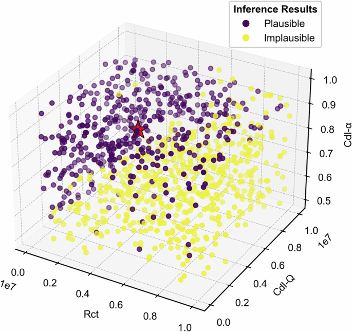
Purple dots: exhibiting well-distributed posterior distributions for all circuit elements; yellow dots: containing poorly distributed posterior distribution for certain elements. Rct: charge transfer resistance, Cdl-Q: magnitude of double-layer CPE, Cdl-α: constant of double-layer CPE. Red mark: the selected EIS data used in the subsequent frequency reduction analysis.
We then used the parameters as input features and the BI results as objectives to build a decision tree and used the tree diagram to better identify the regions of plausibility and implausibility. The model identified the constant (Cdl-α) of the double-layer CPE as the most critical factor, with over 50% of the overall feature importance. As Cdl-α decreases, the capacitive behavior of a CPE as the dominant impedance gradually transfers to the parallel resistor with a smaller fixed resistance. The resistor has a frequency independence to its impedance and therefore the impedance exhibits less response to the frequency changes. This is observed to decrease the plausibility of the given ECM. The second most influential parameter is the value of the charge transfer resistance (Rct), with a lower Rct being more conducive to a successful inference. The decision tree results, as shown in Supplementary Fig. 1, show that a high double-layer constant (Cdl-α > 0.82) combined with a lower charge transfer resistance (Rct < 7.37 × 10⁶ Ω) correlates with successful signal inference. Within this range, around 96.0% of EIS data exhibited statistically plausible inference, indicating that the EIS data can be confidently fit the with associated ECM. By further constraining the value of Cdl-α to be within 0.85–0.98, the success rate increased to 100.0%.
Near the boundaries defined by the decision tree, there are examples of successful and unsuccessful inferences for the ECM components, where one should use with caution. In the regions for which the value of Cdl-α is smaller than 0.76 and Rct is larger than 2.14 × 10⁶ Ω, the BI exhibits a failure rate in excess of 93.6%. Although there are some examples of successful inference within this region, it is recommended to use the ECM carefully as the inference on the EIS is sensitive to changes in the component values. It might be the case that, despite achieving a good fit using the ECM, the reaction signals contained in the data are not strong enough to support a precise parameter estimation upon the ECM.
The impact of reducing the minimum measured EIS frequency on the inference of Cdl-α is shown in Fig. 3. The results demonstrate that we are able to decrease the number of low-frequency measurements taken without degrading the inference up to a threshold frequency. The BI inference is accurate and confident even for a minimum frequency of 0.36 Hz. Supplementary Fig. 2 demonstrates that this holds for all the considered components. Beyond this range the relative error from the mean ground truth value exceeds 4%. This could be considered within experimental error depending on the user’s judgment. It is, therefore, even feasible to exclude additional frequency data at the expense of greater component value uncertainty. As we continue to drop the low-frequency measurements, the mean values of the inferred components begin to deviate more significantly from the ground truth. Eventually, for frequencies >31.6 Hz, the circuit structure becomes non-inferable, containing circuit elements with implausible posterior distributions and noticeable divergences. For this system, the diverged region overlaps with the failed region. The frequency-dependent impedance response for each component in the ECM used to model the system is available in Supplementary Fig. 3.
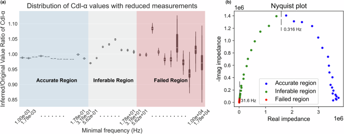
a Violin plot showing the variation in the selected circuit component value (Cdl-α) as low-frequency measurements are progressively excluded. b Nyquist plot illustrating the minimal frequency for regions with different statistical plausibility.
These observations suggest that when performing subsequent EIS measurements during an in-situ degradation study, users would only need to measure the full EIS for the initial state. For subsequent measurements they could skip the low-frequency measurements (<0.36 Hz) and achieve a significant reduction in measurement time (over 99.9%) without detrimentally impacting the integrity of the data analysis. Clearly, the minimum frequency will also be affected by the noise level associated with the EIS measurements, however the proposed method automatically takes the noise into account during its inference. As illustrated in the supplementary materials, a lower noise level allows users to omit even more low-frequency measurements through this framework while ensuring the same analysis integrity.
Passivation of alloys under aqueous conditions
Subsequently, we focused on alloy passivation under aqueous conditions, typically modeled using a Randle circuit with an additional Warburg element to account for a diffusion process. Within the adjusted parameter ranges, we found that most of the generated EIS data failed to yield plausible inference, with only a few successful cases well characterized by a relatively small Warburg impedance (Zw), as depicted in Fig. 4. Failed inferences were identified by straight lines in their Nyquist plots, indicating insufficient signal strength for accurate component value inference. This occurs because as Zw increases, the signal in the absolute sense becomes smaller, but signal from the diffusion and migration becomes significant and dominates the system, overshadowing the charge transfer signal and leading to implausible inferences.
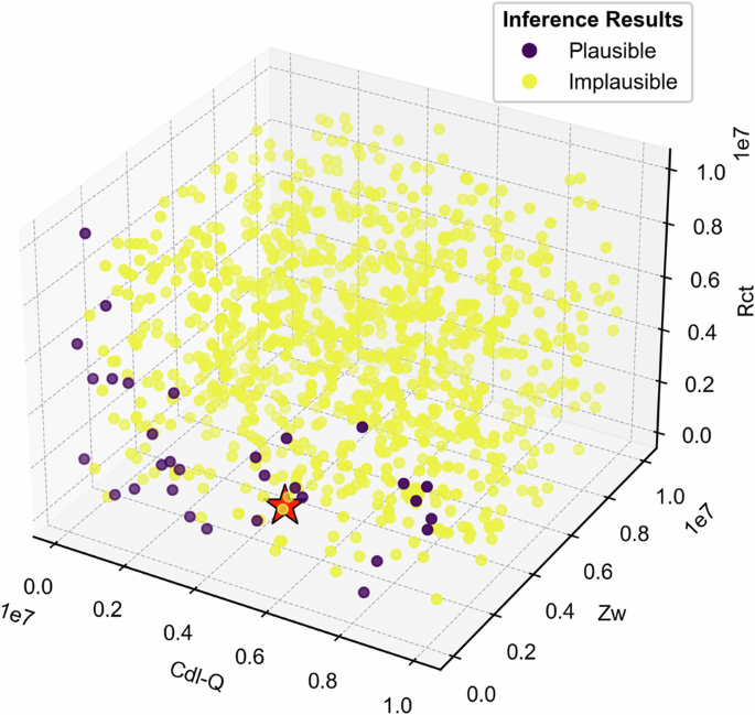
Purple dots: exhibiting well-distributed posterior distributions for all circuit elements; Yellow dots: containing poorly distributed posterior distribution for certain elements. Cdl-Q: magnitude of double-layer CPE, Zw: Warburg impedance, Rct: charge-transfer resistor. Red mark: the selected EIS data used in the subsequent frequency reduction analysis.
Similar to the above, we built a decision tree model using the component values and BI results, as visualized in Supplementary Fig. 4. According to the model, the magnitude of the Warburg element (Zw) was identified as the most influential factor, weighing over 85% of the feature importance. For values of Zw lower than 1.03 × 10⁶ Ω s-α, over 3.9% of EIS data exhibited plausible inference, while all EIS data encountered failed inferences with a Zw larger than this value. The second influential parameter is the magnitude of the double-layer CPE (Cdl-Q). In regions where Zw is smaller than 1.03 × 10⁶ Ω s-α and Cdl-Q is larger than 2.89 × 10⁶ Ω s-α, the BI failed for all EIS data.
Figure 5 illustrates the effect of the frequency reduction on the inference of Zw using the selected EIS data. The results show that the inferences on Zw remained both accurate and confident within a 4% relative error compared to the ground truth down to 0.01 Hz. The inference on other ECM components also remains accurate with less than a 4% relative error, as shown in Supplementary Fig. 5. Beyond this range, the error exceeds 4%, which may still fall within acceptable limits depending on user judgment. Despite the increased uncertainty, the resulting reduction in measurement time is significant (over 90% of the total measurement duration).
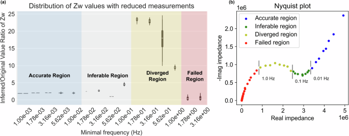
a Violin plot showing the changes in the selected circuit component value (Zw) as low-frequency measurements are progressively excluded. b Nyquist plot illustrating the minimal frequency for regions with different statistical plausibility.
The inference maintains its confidence until 0.1 Hz, after which a large number of divergences occur in conjunction with a substantial increase in the relative error, marking a decreased model reliability. Although the posterior distributions of circuit elements remain well-centered, it is recommended to use the ECM with caution for this range of frequencies. For frequencies above 1.0 Hz, inferring the circuit structure becomes impractical with implausible posterior distributions for circuit components. The individual contributions of each circuit element in this ECM across the measured frequencies are detailed in Supplementary Fig. 6.
Coated metal corrosion systems
The BI results of the coating system are depicted in Fig. 6. The data in this figure suggests that a relatively smaller pore resistance (Rpo) is beneficial in obtaining plausible BI results within the specified ECM. As the pore resistance increases, the inference results exhibit less robustness to noise.
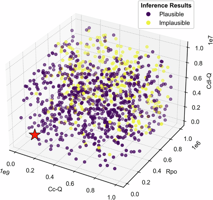
Purple dots: exhibiting well-distributed posterior distributions for all circuit elements; Yellow dots: containing poorly distributed posterior distribution for certain elements. Cc-Q: magnitude of coating CPE, Rpo: pore resistance, Cdl-Q: magnitude of double-layer CPE. Red mark: the selected EIS data used in the subsequent frequency reduction analysis.
After training a decision tree model using the adjusted parameters and BI results, the pore resistance (Rpo) was identified as the most significant factor for successful inference, accounting for ~45% percent of the feature importance. The decision tree results (as shown in Supplementary Fig. 7) indicate an initial separation when the pore resistance (Rpo) exceeds 4.54 × 10⁵ Ω. EIS data with Rpo below this threshold exhibit plausible posterior distributions in over 89.3% of cases, suggesting sufficient signal to substantiate the given circuit structure.
The influence of frequency reduction on the inference of the magnitude of Warburg element (Zw) is demonstrated in Fig. 7. For the selected EIS which features two semi-circles, omitting low-frequency measurements below 0.018 Hz has a negligible impact on the inference accuracy on Zw with less than a 4% error but reduces over 94.3% measurement time. Other ECM components also retain this level of accuracy, as demonstrated in Supplementary Fig. 8. Utilizing BI with impedance data above this threshold, users retain the capacity to confidently infer component parameters while the error exceeds 4%. Furthermore, BI can reliably suggest the ECM structure up to the point where all frequencies below 0.18 Hz are excluded, after which divergence emerges in the inference results and it marks a decreased EIS-ECM pair alignment. After removing measurements below 1.0 Hz, the ECM structure becomes non-inferable. The frequency-dependent impedance response for each component in the ECM used to model the system is available in Supplementary Fig. 9.

a Violin plot showing the changes in the selected circuit component value (Zw) as low-frequency measurements are progressively excluded. b Nyquist plot illustrating the minimal frequency for regions with different statistical plausibility).


Responses