Bayesian estimation of the likelihood of extreme hail sizes over the United States

Introduction
In the past decade, increasing insured losses from hail have been in part driven by multiple large single-city loss events exceeding USD 1 billion, including Denver, Minneapolis, Dallas, Phoenix, and Oklahoma City1,2,3. Hail is a frequent hazard across the United States, with hail in excess of 25 mm in diameter (1 inch) frequencies exceeding one event per year for areas on the scale of 1° × 1°, with a maximum in the Great Plains4,5,6,7. The size of hail varies across the country. Hailstones (>45 mm, >1.75 inches) that unassisted are capable of producing damage to structures and property are more common in the Great Plains but become increasingly rare in the Midwest and Northeast, whereas they are comparatively uncommon in the west of the Rockies8. This variation in size and frequency over the continent means that the return periods can be variable. However, while the broader scale return intervals imply relatively frequent hail of large sizes, it is less clear how this translates to smaller scales, for example, the area of an individual city. Similarly, while prior work has relied on the Gumbel distribution over southern France, the US and China respectively to describe the hail hazard8,9,10, the fitting of the Gumbel distribution was noted to be primarily a function of insufficient data being available to fit the shape parameter of a Generalized Extreme Value (GEV) distribution. To address this limitation, here we focus on using the spatial inconsistencies of hail data to our advantage while leveraging multiple available data resources to identify a more robust quantification of observed hail return intervals through appropriate functions and fitting mechanisms for estimating hail risk.
Hail observational data have a number of limitations, ranging from the sporadic and inconsistent nature of reporting11, non-meteorological discontinuities associated with changes to warning practices12, to spatial variations in reporting frequency that can lead to biases towards cities and roads8, and incomplete representation of the size distribution7. While prior analyses have sought to address these through arbitrary smoothing using isotropic Gaussian functions or local area weighting [e.g. refs. 8,13,14], this approach treats all grid points equally, which climatologically is not a true reflection of the way these data are observed. For example, SPC storm data is a dataset built focused on warning verification, contains few reports less than 19 mm (0.75 in.), and is typically biased toward more highly populated or at the least heavily traveled areas11. Recent work by Elmore et al.7 illustrated how incomplete this size record is from an observational standpoint, and pointed out the value of including additional observations from mPING15 and CoCoRAHS16 data to produce a climatology of both sub-severe and severe hail. While the spatial biases remain problematic for building a national return size map, through combining datasets there is clear evidence that a more representative rate of occurrence for hail can be obtained.
It could also be argued that this spatial bias should not always be considered to be without value. For example, there is evidence that the number of hail observations is very high and might be approaching a low likelihood of being missed in urban areas, an apparent saturation. This is particularly evident in cities [e.g. Dallas, Wichita and many populated areas in Switzerland12,17,18], as well as across the Continental United States11. Rather than focus on resolving this bias, which is a challenging way to address the true observational frequency of severe weather events for hail [e.g. ref. 19], we instead use the information from these well-observed locations to fit extreme value distributions and use a coarse representation of frequency to subsequently inform parameters for a high resolution gridded climatology of hail risk over the United States. The reliance on observations is partly driven by the limitations of other remotely sensed techniques such as radar or satellite proxies. Unfortunately, while these remotely sensed data can tell us much about the recent frequency of hail events5,6,20, they remain a proxy estimate that is unreliable for hail size21 and are generally limited to comparatively shorter periods than would be desirable for estimating return intervals.
The motivation for this analysis is driven by the absence of hail as a design risk category within current standards22. Given increasing vulnerability in building materials and property17,23, which now include high-value utility-scale photovoltaic installations in areas where hail is more prevalent24, there is a need to develop an accurate risk assessment of hail that can inform design standards. In prior work8, the distributions used were constrained by the poorest available data restricting the fitting procedure, however, it was recognized that this may not reflect the optimal way to describe the underlying hail hazard. For example, unresolved questions remain for the underestimation of smaller magnitude but frequent events, a known characteristic seen in environmentally-derived approaches4, observational climatology7 and radar-derived analyses5. These imply that an assessment of the reliability of fit obtained using an annual maximum is prudent. To address these research challenges, we seek to answer 3 specific questions:
-
1.
What is the best approach to characterize the functional form of the return interval curve where observations are sufficient to make such estimates?
-
2.
How do we reconcile spatial biases in estimating a complete hazard map for hail?
-
3.
What is the effective hail exposure to urban centers around the US and does this indicate ”hotspots” of risk?
Results
GEV distribution based on MLE
To provide a baseline and use a fitting approach analogous to previous methods, we first fit the 0.25° × 0.25° resolution annual maximum hail size gridded data with a GEV distribution through the Maximum Likelihood Estimation (MLE) technique. Fitted locations are informed by the observational frequency of hail at the resolution of 0.25° × 0.25°, with at least 15 annual maxima for the analysis period required (Fig. 1). We obtain the estimated parameter values along with their 95% confidence intervals for location, scale, and shape parameters of GEV distribution over the continental United States (Fig. 2). The estimated values of location, scale, and shape parameter represent the central tendency, dispersion and tail behavior of the distribution of annual maximum hail size respectively (Supplementary Fig. 1), and their 95% confidence intervals indicate the uncertainty associated with the parameter estimation process. Fitting through this approach we see that even at this relatively fine grid scale there is considerable variability in the fit, with location parameter ranging from 0.4 to 1.86, the scale parameter ranging from 0.09 to 1.03 and shape parameter ranging from −1.1 to 1.29. The lack of consensus in shape parameters also suggests that the three-parameter fitting approach is leading to varying results compared to earlier methods8. While the estimated shape parameter values are less than zero for around 76% of the considered grids, around 96% of grids have negative shape parameters for the lowest confidence interval. This result suggests that while fitting may be influenced by the volume of available data, the distribution converges toward a bounded upper tail for the hail size distribution. With finite upper limits, extreme events become less likely as magnitude increases25. In this study, the large hail(hail size > 0.75 inch) is classified as severe (0.75inch < hail size < 1.5 inch)12,26, 1.5–3 Inch (38–76 mm), and 3+ Inch (hail size > 3 inch, > 76 mm).

a Total number of years of hail occurrences. b Maximum of annual maximum hail size.
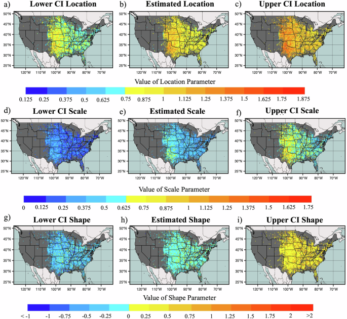
a–c represent the lower, estimated, and upper 95% confidence interval of the location parameter respectively. d–f represent the lower, estimated, and upper 95% confidence interval of scale parameter respectively, and g–i represent the lower, estimated, and upper 95% confidence interval of the shape parameter.
Generally, across the Great Plains states the scale parameter tends to have higher values, with around 29% of grids greater than 0.5 across the Great Plains states, particularly over Texas, Oklahoma, and Kansas. This indicates that the occurrence of large hail size is more widespread in this region. Most of the central and eastern US tend towards relatively lower scale parameter values at around 70% of grids, indicating less dispersion in the distribution for large hail. In contrast, higher location parameters are found over a broader area, except for the southeastern United States. Similar to scale, the location parameter is found to be comparatively higher across broader areas including Texas, Oklahoma, Kansas, Nebraska, and South Dakota. This signifies a greater likelihood of encountering larger hail sizes surpassing the higher threshold of large hail in this region. While around 62% of considered grids over the US have location parameters greater than 1, approximately 38% of grids are less than 1. Both location and scale parameters exhibit higher values over larger areas with extreme hail size i.e., 3+ Inch hail in the Great Plains (Fig. 2). Finally, shape parameters for this approach are negative, which indicates the tail behavior of the distribution of hail size, revealing that a large area experiences a tailing behavior toward lower probabilities of 3+ Inch hail size. In contrast, few grids with positive shape parameters are sparsely distributed across the United States. An attribute common for all parameters is the high degree of uncertainty from the MLE fitting approach.
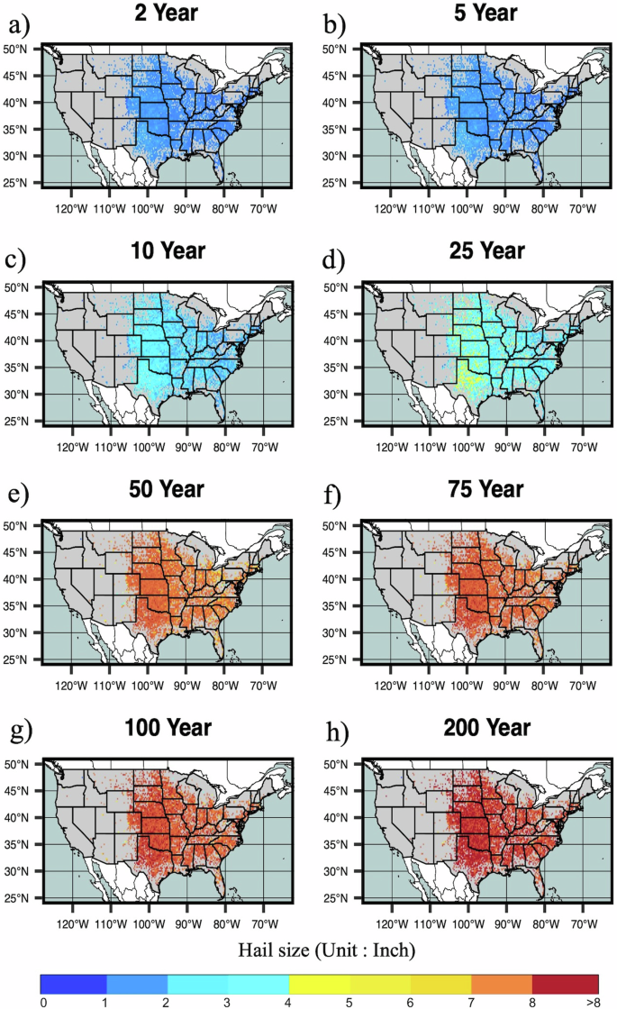
To further evaluate model performance, return levels were used to explore the frequency and magnitude of rare hail events. Return intervals at the 2-year period (50th percentile), reflect 88 percent of fitted grids being affected by severe hail occurrences (Fig. 3). Extending to 5 to 10-year return intervals, an increasing number of grid points experience 1.5–3 Inch hail, while at 25–50-year intervals 3+ Inch hail is more common, particularly over the Great Plains. Overall, the GEV distribution highlights larger hail sizes than prior work using the Gumbel distribution, even considering the finer grid size8. As return intervals extend to 200-year intervals, around 37 and 62 percent of the considered grids are affected by 1.5–3 Inch hail and 3+ Inch hail sizes respectively.
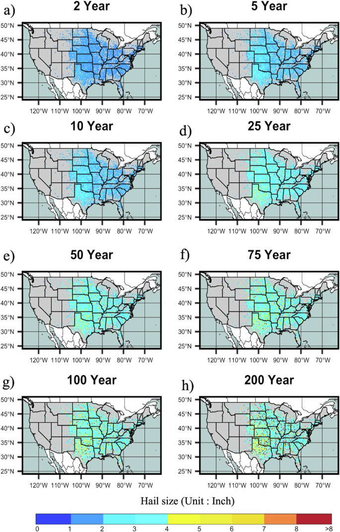
Modeled hail size return intervals are shown for a 2-, b 5-, c 10-, d 25-, e 50-, f 75-, g 100-, h 200- year return periods.
Bayesian modeling using informative priors
To better represent return intervals, we next test an approach leveraging inferences from Bayesian priors. We obtain informative priors from the past hail record of 1° × 1° resolution to reduce the uncertainty in the initial guess for parameters of the GEV distribution and thereby enhance the computed hail return levels. Rather than presenting this information as a grid-by-grid estimate, instead, at each 0.25° × 0.25° resolution grid, the informative priors of location, scale, and shape parameter of GEV remain consistent. Based on this approach, informative priors are provided in clipped distributional forms as follows
where α, β denotes the shape and rate parameter of gamma, and μ, σ are the mean and standard deviation of normal distribution.
Subsequently, fitting a Markov-Chain Monte Carlo approach with the Metropolis-Hasting recipe27 was considered to generate the samples from posterior distributions. From this, the posterior means, standard deviation, and confidence intervals for each GEV distribution parameter were computed for each grid. Posterior estimated parameter values and their 95% confidence intervals illustrate that estimated values of location varied from 0.51 to 1.77, reducing the parameter range compared to the MLE method (Fig. 4). Estimated value ranges for scale (0.21 to 0.79) and shape (−0.38 to 0.73) parameters are also narrowed, particularly for the shape parameter, which skews the distribution toward positive values (Fig. 4). These suggest that the Bayesian prior approach provides considerable value in reducing the uncertainty of each parameter in the GEV distribution, and as a result, provides more reliable insight into the hail hazard. Evaluation of the differences (Supplementary Figs. 2 and 3), indicates that the largest variations between MLE and Bayesian fitted parameters occur where the number of hail observations is limited, and hence confidence in the distributional fit decreases, while at well-observed locations estimated adjustments are smaller.
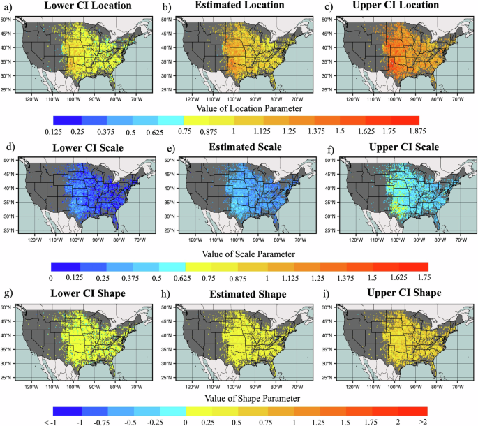
a–c represent the lower, estimated, and upper 95% confidence interval of the location parameters respectively. d–f represent the lower, estimated, and upper 95% confidence interval of scale parameter respectively, and g–i represent the lower, estimated, and upper 95% confidence interval of shape parameter.
In some regions, parameters are adjusted considerably relative to the MLE approach (Figs. 2 and 4). Across the Great Plains states, particularly over Texas, Oklahoma, and Kansas, the majority of grid points exhibit location parameters within a range of 1.125 and 1.375 based on MLE, the Bayesian gives the range of 1.5 to 1.75. Given the location parameters are linked to the size expected at a given return interval, this implies that the MLE approach systematically underestimates the relative risk with increasingly long return intervals. This is particularly prevalent where the hail frequencies are fewer, but larger stones are possible at longer return intervals, as seen over the eastern United States. In contrast, scale parameter estimates show less sensitivity to the MLE vs the Bayesian approach, suggesting that the rarity property is captured using either method. Consistent with physical expectations, this implies that while the central tendency of hail was underestimated in prior MLE approaches, the potential bounds for the variability of hail size do not significantly differ across the United States based on both Bayesian and MLE approaches. Shape parameters show the greatest sensitivity to the method used, with nearly all grids showing a consistent positive parameter value, contrasting the mixed sign found for MLE (Fig. 4). This suggests that a primary value of the Bayesian approach comes in the tailing behavior of the distribution, and highlights that the extreme values of the tail were underestimated in the MLE.
Directly comparing the methods based on RRMSE and RAE, we assess the performance of the estimation technique within specified quantile ranges (Fig. 5, Supplementary Fig. 4). This highlights that at lower quantiles, the MLE tends to produce better RRMSE and RAE than the Bayesian approach whereas at higher quantiles, Bayesian tends to outperform MLE. Explanations for this difference likely reflect sensitivity to prior information, model flexibility, the robustness of the Bayesian approach, the role of sample size, and model complexity. In the context of sensitivity to prior information, in our study, one driver could be the sparsity of hail data at a lower quantile in 1° × 1° resolution data. This can lead to weaker informative prior at lower quantiles. On the other hand, in 0.25° × 0.25°, there is comparatively better hail information at lower quantiles. This causes the performance of MLE better than Bayesian at lower quantiles in 0.25° × 0.25° as MLE mostly relies on the observed data. At the same time, this result is also consistent with results seen in other studies which demonstrate that the Bayesian technique is generally considered more robust in handling outliers and extreme values due to its ability to incorporate prior knowledge28,29,30.
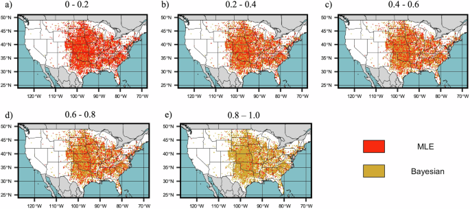
This illustrates the better estimation technique based on RRMSE value at different quantile ranges of annual maximum hail size for the grids having at least 15 annual maximum hail size observation at 0.25° × 0.25° resolution. The quantile ranges are taken for a 0–0.2, b 0.2–0.4, c 0.4–0.6, d 0.6–0.8, e 0.8–1.
Influence of priors on return levels
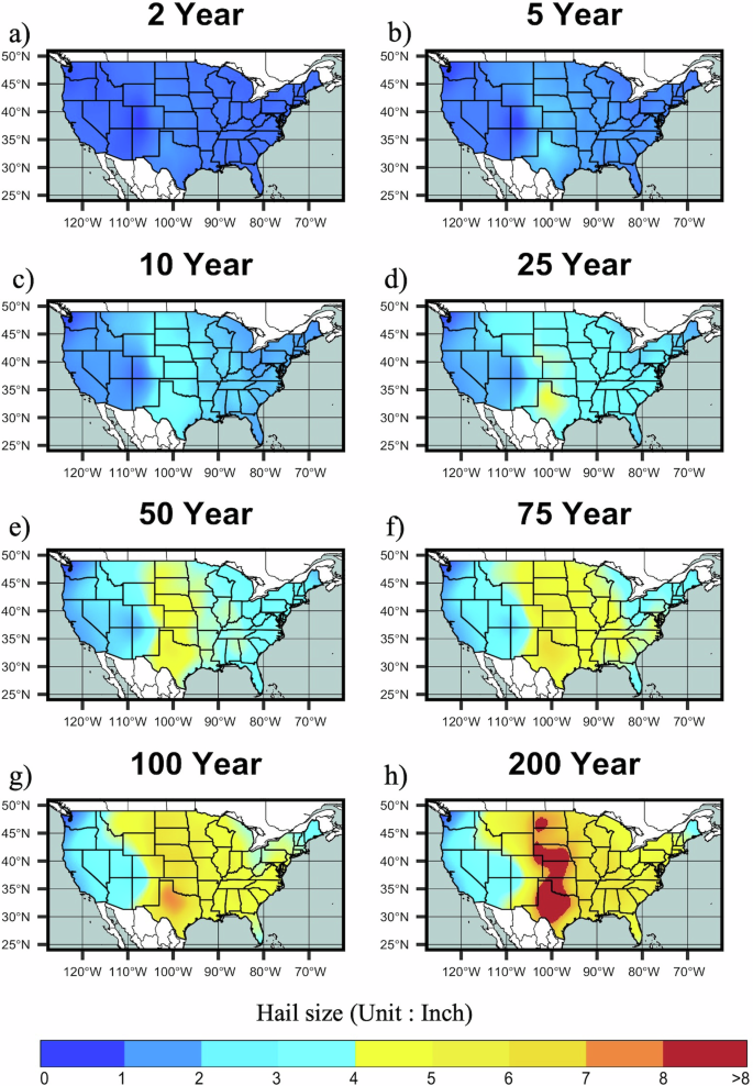
Having established the reduction in uncertainty and consistency of the return intervals from the Bayesian approach, we consider the resulting return intervals (Fig. 6). Posterior densities at the respective grids indicate slightly smaller sizes at the shorter return intervals, with 51–76 mm (2–3 inches) hail more prevalent at the 10-year return interval, contrasting this signal at the 5-year level for the MLE approach (Fig. 3). At the 25-year return interval level, distributional estimates for both the MLE and Bayesian approach are comparable (Figs. 3 and 6). In contrast, with increasing return periods, estimated sizes grow more rapidly in the Bayesian approach, with the 100-year values in the MLE being closer to the 50-year return. By the 200-year return, sizes for the Bayesian estimate over the Great Plains generally approach the maximum observed sizes in the historical record at 203 mm (8 inches)8.
Modeled hail size return intervals are shown for a 2-, b 5-, c 10-, d 25-, e 50-, f 75-, g 100-, h 200- year return periods.
The nature of the observed record results in spatial distributions that are incomplete representations of the hazard frequency. To address this issue, we leveraged an adaptive Gaussian Process Regression (GPR), with an anisotropic Matern kernel to smooth this incomplete picture into continuous return maps (Fig. 7). Smoothing was performed on the location, scale, and shape parameters respectively, to avoid potential smooth issues arising from larger value variance in the return mapping, and to deal with differences in the relevant anisotropic length scales, variance, and noise (Supplementary Fig. 5). As the GPR technique also provides confidence intervals of the fitted distributions, this can be used spatially to highlight areas where the fitted distribution has less or greater uncertainty (Supplementary Fig. 5). Comparison between the smoothed and native fitted returns suggests minimal bias for location and scale, however, smoothing the shape parameter tends to shift the distribution toward a value of 0.35 (Supplementary Fig. 6). Resulting return maps (Fig. 7) highlight peak values for hail size extending from Texas through to North Dakota, with a westward extension into eastern Colorado, Wyoming, and Montana, consistent with remotely sensed climatologies of frequency5,6, and favorability for severe thunderstorm development31. In the eastern part of the country, higher magnitudes are found across the Midwest south of the Great Lakes, and through the southeastern states, with these peaks split by the high topography of the Appalachians. Despite this smoothing procedure, the Appalachian discontinuity may reflect persistence of undersampling of observations into the fitted and subsequently smoothed model, as low population impacts reporting frequency in this region4 despite ample evidence of supercells producing hail in this region32. Overall return values of hail size are not as extreme as for the grid box calculated parameters, which reflects the effective local weighting of parameters to constrain grid boxes with greater uncertainty or largely anomalous parameter values. Despite relatively sparse fitted data, Arizona’s comparative risk suggests that the 76 mm (3 inches) hail produced during the 2010 record hailstorm would be consistent with a 200-year annualized return interval event.
Modeled hail size return intervals are shown for a 2-, b 5-, c 10-, d 25-, e 50-, f 75-, g 100-, h 200-year return periods.
To assess the impact of large hail occurrences in urban areas, we have examined the fitted return intervals for 12 specific cities across the United States (Fig. 8). Here, we compared the return curves from three techniques i.e., MLE, Bayesian, and smoothed Bayesian through GPR. For each technique, we have also taken the return intervals from the 95% confidence interval. It is apparent that for low return intervals, i.e., up to a 2-year return period, there are only small differences in hail size among the three. However, the hail return curve of the Bayesian approach starts deviating from the MLE return curve after the 2-year return interval, and the deviation keeps increasing as the return period increases. This suggests a significantly higher hail return level in Bayesian compared to MLE indicating relevance of prior information in limited observation applications such as hail data. At higher return periods, while MLE shows the probability of 1.5–3 Inch hail occurrences, the Bayesian approach reveals 3+ Inch(≥76 mm) hail occurrences at the 40-year return period.
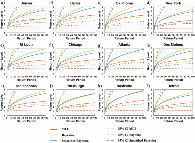
The return interval curves are shown for a Denver, b Dallas, c Oklahoma City, d New York, e St Louis, f Chicago, g Atlanta, h Des Moines, i Indianapolis, j Pittsburgh, k Nashville, l Detroit.
However, for New York, Atlanta, Pittsburgh, and Nashville, differences between the Bayesian and GPR smoothed return curves show much smaller differences. This suggests that part of the fitting instability that leads to differences in locations where larger hail is more prevalent is related to the more extreme values at the tail in the nearby vicinity of the locations. These results highlight that the chosen kernel functions and hyper-parameters of the Gaussian process are appropriate for capturing the underlying structure of data including noise, and appropriately compensate for regional structures in hail size data. Among these cities, the highest return rates are found for Dallas and Oklahoma City which both have ≥127 mm (≥5 inch) hail return levels at 50-year return periods.
Spatial analysis of population exposure and hotspot identification
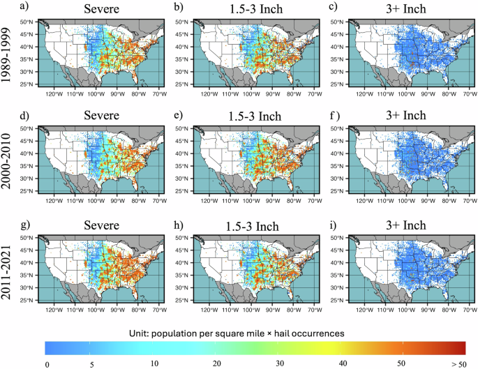
While hail event frequency can provide useful insights, the intersection of frequency and heavily populated areas dictates the risk. To investigate the areas with the highest risk, we use population density and hail occurrences in the last three decades to calculate the decadal population exposure. To provide the hazard basis for this analysis, we combine the spatial frequency of hail events stratified into size categories (Fig. 9). Across the 5148 grids with at least 15 years of observations, 1007, 3064, and 1805 grids have experienced severe hail events more than 5 times in each of the last 3 decades respectively. This expands to around 43%, 50% and 45% percent of the grids experiencing at least two 1.5–3 Inch hail occurrences during 1989–1999, 2000–2010, and 2011–2021 respectively. Whereas there are few grids that have experienced at least one 3+ Inch hail occurrence during 1989–1999 (40), 2000–2010 (35) and 2011–2021 (58) respectively. This frequency analysis highlights the hail risk over the Great Plains, especially over Texas, Oklahoma, and Kansas all of which have experienced from severe to 3+ Inch hail occurrences in the last three decades. Moreover, in small portions of New Mexico, Wyoming, and Montana, and a comparatively larger portion of Colorado, severe and 1.5–3 Inch hail have been a frequent visitor. Outside of the Great Plains, the southeastern and some portions of the eastern part of the United States have also been affected by severe and 1.5–3 Inch hail occurrences. Intriguingly, there is evidence of decadal variability in the occurrence of severe and 1.5–3 Inch hail in comparing the period 2000–2010 to 2011–2021, which may reflect responses to natural climate variability [e.g. ref. 33]. An increasing number of locations have recorded 3+ Inch hail in the recent decade, extending as far east as Alabama to Illinois, and westward from Texas to the Dakotas. We caution that as such events are likely under-recorded12, this signal is likely driven by non-meteorological factors, but supports increased confidence in the reliability of the Bayesian fitted distributions.
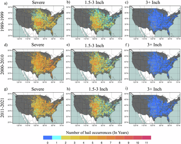
a–c are shown for severe, 1.5–3 Inch hail, and 3+ Inch hail occurrences respectively during 1989–1999. Similarly, d–f represent severe, 1.5–3 Inch hail and 3+ Inch hail occurrences respectively during 2000–2010, and g–i represent severe, 1.5–3 Inch and 3+ Inch hail occurrences respectively during 2011–2021.
As the distribution of population does not coincide with that of the occurrence of hail hazard (Fig. 10), we explored hail risk through a combined analysis. This highlights that while hail is more prevalent in the Great Plains, the exposure factor in severe (19–38 mm) and 1.5–3 Inch hail (38–76 mm) is predominantly in the eastern United States, and has been increasing, in line with population increases and urban sprawl, consistent with the effects noted by Childs et al.34 and Strader and Ashley35 regionally and for other severe weather hazards. Despite less frequent hail occurrences, high population densities contribute to significant population exposure to severe and 1.5–3 Inch hail occurrences. In densely populated regions, even rare occurrences of hail can lead to substantial property loss due to the concentration of valuable assets and infrastructure. However, some regions of Texas, Oklahoma, Kansas, Nebraska, Arkansas, Missouri, Iowa, Minnesota, Mississippi, Alabama, Tennessee, Wisconsin, Ohio, and Florida also experience less frequent 3+ Inch hail over very highly populated areas. Furthermore, compared to the east, a few grids from New Mexico, Arizona, Colorado, and Montana are under high population exposure due to lower population.
a–c indicates the population exposure under severe, 1.5–3 Inch and 3+ Inch hail occurrences during 1989–1999. d–f indicates the population exposure under severe, 1.5–3 Inch and 3+ Inch hail occurrences during 2000–2010, and g–i indicate the population exposure under severe, 1.5–3 Inch and 3+ Inch hail occurrences during 2011–2021.
As a final application of these insights, we have utilized a combination of frequency of severe and 1.5–3 Inch hail, return levels, and population density to delineate a set of hotspots across the U.S.(Supplementary Fig. 7). To qualify as a hotspot, we have considered the population density greater than 100 people per square mile, at least two severe hail occurrences (at least once for 1.5–3 Inch) in the most recent decade, and having severe or 1.5–3 Inch hail return levels at 25-year return period. This analysis captures the most susceptible hail-prone areas. Several grids in Nevada, Arizona, Colorado, North Carolina, Georgia, and Virginia, and many in Texas and Illinois, Ohio, and Florida along with border regions between Kansas and Missouri emerge as significant hotspots where population, return likelihood, and severe and 1.5–3 Inch hail occurrences align. These locations, generally characterized by dense population density can be particularly vulnerable to substantial economic losses. However, Oklahoma presents a contrasting scenario. Despite experiencing relatively higher hail returns, due to lower population density this constrains the potential for the largest economic losses due to hailstorms. Over the highly populated eastern United States Boston, Washington D.C., New Jersey, and Annapolis areas are also identified as hotspot regions under severe and 1.5–3 Inch hail occurrences, driven predominantly by population and return interval. These results suggest that efforts to mitigate hail damage should not only focus on where large hail has the greatest frequency.
Discussion
Hail-insured and uninsured losses and their associated risk are an increasingly prevalent problem across the United States. Leveraging insights from prior analyses, and all available hail observational data, we have characterized hail through smoothed hazard maps that are aimed at underlying future design standards. We also illustrate that prior estimates likely underestimated the hazard posed by hail and that despite data limitations, techniques such as extreme value analysis can be applied to hail data. This underestimation is the result of two factors; the prior grid size not representing locations where observations were more frequent, and the underlying distributional assumptions not being suited to the application.
The resulting distributions address many of the uncertainties that arose from the use of the Gumbel distribution in prior analyses [e.g. ref. 8]. This was accomplished by enhancing our modeling approach using a Bayesian estimation through the GEV distribution which provides a better functional form to estimate hail return levels. This reduces uncertainty and shows that return levels from the Gumbel distribution likely underestimated rarer events. The method proved robust even with limited observed data in specific locations. Complementing this, we also provided a comprehensive spatial estimate leveraging an adaptive GPR machine learning smoothing technique. The flexibility of GPR in modeling complex and anisotropic patterns significantly enhanced our ability to extrapolate from the underlying sparse datasets, thereby creating a detailed nationwide dataset of returns that is needed for standards maps. The GPR technique in particular contrasts inflexible smoothing approaches used in prior studies and illustrates that this type of smoothing could be used effectively for other spatially incomplete hazards.
The success of the analysis here argues for a more adaptive approach to working with severe weather data; uncertainty and non-uniformity can be used in novel ways to address and overcome the limitations of observational approaches. These results also guide how risk analysts should contextualize hail risk. Especially at small sample size grids, Bayesian techniques enable the risk analyst to comprehensively account for the uncertainties in hail return level estimates, empowering them to make more informed decisions with greater confidence. Furthermore, while the hazard analysis identifies the regions prone to large hail, we note that hail risk is contingent upon factors like population density and frequency of hail occurrences along with hail return levels. By exploring the population exposure changes for different categories of hail size for the last three decades, we are able to illustrate that much of the hail risk is driven by exposure, not necessarily changes to hail, a result noted by ref. 36 and found for other severe weather hazards35. This nuanced approach offers richer insights into societal vulnerabilities and potential impacts associated with varying magnitudes of hail.
The pattern of hail hazards highlights extensive areas across the central and eastern United States are exposed to extreme hail size, which is particularly pronounced under Bayesian estimation in higher return periods. Likewise, the population exposure further underscores elevated risk in specific locations, aligning with regions experiencing notable losses in recent years. Especially, the rise in the frequency of damaged and 3+ Inch hail occurrences in recent past two decades compared to the period from 1989 to 1999, serves as a stark warning regarding the potential for heightened exposure to losses caused by damaged and 3+ Inch hail. Thus combining the exposure, hail occurrences, and hail returns effectively identifies the hotspots of hail risk across the U.S. By highlighting these hotspots, we aim to encourage mitigative efforts and enhancements to building resilience for many areas outside of those traditionally thought of as severe weather states.
However, while this study demonstrates advancements in estimating hail return levels using GEV with a Bayesian estimation technique, we acknowledge that there are limitations to these methods and propose strategies for addressing them in future research. The assumptions underlying the GEV model and Bayesian estimation approach, such as stationarity and prior distribution specifications, may not always align with the dynamic and complex nature of hail events. To mitigate these limitations, future research could explore alternative approaches for refining model assumptions around these assumptions. One approach to do so is the integration of environmental covariates to enhance the predictive capability of this model, particularly in poorly observed areas, and thereby provide more accurate estimates of hail return levels and reduce uncertainty. While prior approaches have addressed hail frequency above defined size thresholds through covariate modeling [e.g. refs. 4,37,38], these have mostly focused on keeping environmental parameters that are relevant at the daily or monthly scale. Building on this, we believe it is possible to develop a covariate-based model for the GEV parameters of the hail size distribution to estimate the return levels by considering distributional environmental properties. This type of approach will allow quantification of regions where observations may be understating risk and enhance our ability to evaluate the return levels of hail occurrences, thus leading to improved hail risk management strategies across the U.S. both now and in the future.
Methods
Hail data
To construct a record of hail observations, mPING15, CoCoRaHS16 and Storm Prediction Center (SPC) storm reports were utilized, reflecting the all available hail size data7.mPING data is available from 2012–2021, CoCoRaHS data is from 2003 to 2021 and SPC data spans from 1979 to 2021. The resulting dataset combining these three sources is 406,753 hail reports spread across the United States. Ensuring a representative record is important for extreme value theory, where the number of observations can affect the accuracy of the fit. While the availability of hail data is not consistent through time, reporting practices have evolved over the years with significant improvement in the late 1980s and 1990s due to increased public awareness and formalization of the NWS storm spotter program11.
Quality control of data involved the removal of all reports with no size information and filtering the records as in ref. 8, and then gridding to an Albers equal area projection on 0.25° by 0.25° and 1.0° by 1.0° grids respectively. The data were sorted by date of observation and by size, ensuring that the largest hail stone for each date was retained, thereby filtering for annual maximum hail size at each grid. Using the gridded climatology, the number of annual maxima, mean hail size and maximum hail size was calculated for each cell for the entire 1979–2021 period (Fig. 1). Analogous to the approach used in ref. 8, for each observation, a random uniform distribution perturbation was applied to each hail observation to allow for the known mis-characterization of hail size11. This approach also alleviates the quantization issue that arises for hail reports for validating extreme value models8. This allows for more robust estimates of fitted return intervals.
Modeling extremes and generalized extreme value distribution
Extreme value theory is used to quantify the stochastic behavior of unusual rare events and model the large hail size39. We fit the generalized extreme value (GEV) distribution to the annual maximum hail size data from 1979 to 2021 and evaluate the location, scale, and shape parameters at each grid. The GEV distribution can follow the Weibull, Gumbel, and Frechet distributions based on negative, zero, and positive value of the shape parameter respectively40. Moreover, the behavior of the GEV distribution’s tail depends on the value of each parameter (Supplementary Fig. 1). Specifically, the positive shape parameter results in a distribution with a heavy tail on the right (more extremely high values), while a negative shape parameter results in a distribution with a light tail on the right (fewer extremely high values). GEV has several limitations, for example, the assumption that the underlying events are independent of each other and come from the same distribution. In meteorological data, this assumption may not always hold true due to the diverse nature of hailstorm events. The largest hailstones can come from different storm modes and there is variation in the underlying physical processes of hail formation25. Despite not fully satisfying the assumptions, the GEV can still be valuable for hailstorms due to its robustness and flexibility in a wide range of shapes including heavy tails and skewness. GEV also requires the estimation of a shape parameter, which depends on higher order moments of the distribution, and is challenging to estimate and often highly variable, but can strongly affect the upper tail of the distribution [e.g. ref. 41]. The GEV distribution can be defined in Eq. (1) as follows:
where x represents the annual maximum hail size and θ represents the three parameters (μ, σ, ξ) of the GEV distribution. μ, σ, ξ denote the location, scale and shape parameters respectively.
To ensure fitting only uses a robust observation record, only grids with greater than or equal to 15 years of hail size data are considered for the analysis. However, along with choosing the appropriate distribution for a given problem, it is also of paramount importance to select an appropriate parameter estimation technique, as this can greatly impact the resulting distribution, as fitting is sensitive to the type of data and nature of the quantity being estimated.
Parameter estimation technique
Previous studies have examined the effects of different estimation techniques on GEV parameters for climatic extremes. Hossain et al.42 investigated four estimation techniques i.e., ML, GML, Bayesian, and L-moments, and revealed that the length of data series has a significant impact on GEV distribution parameters. When dealing with large samples, a similar type of trends were observed for different estimation techniques. However, the ML method, while offering a straightforward approach, may struggle to adequately address uncertainty, especially with smaller sample sizes. This limitation arises because ML relies on an asymptotic normality approximation of the maximum likelihood estimator, as highlighted in previous studies39,43. On the other hand, the Bayesian estimation method provides a consistent and complete description of uncertainty in extremes28,29,30. Therefore, in this study we consider both MLE and Bayesian estimation technique to investigate their significance in estimating the GEV distribution parameters and hail returns.
Maximum likelihood estimation (MLE)
Considering the annual maximum hail as identically distributed from a GEV distribution, the log-likelihood function of GEV distribution is defined (in Eq. (2)) as follows39:
where θ = (μ, σ, ξ) and ({y}_{i}=left[1-(xi /sigma )({x}_{i}-mu )right]). Then the location, scale, and shape parameters can be obtained by partial derivatives of the log-likelihood function based on the Newton-Raphson method. For a quantile xp with a non-exceedance probability of p, the maximum likelihood estimator can be calculated by Eq. (3):
where ({hat{x}}_{p}) is the inversion of the GEV distribution. In this study, the Maximum Likelihood estimation method is considered to estimate the parameters of the GEV at 1° by 1° to extract priors and also at 0.25° by 0.25° resolution hail size data.
Bayesian estimation technique
In climatic extremes, uncertainty analysis should be taken into account when estimating extreme quantiles due to large sample variance. The ignorance of such variance can lead to significant mischaracterization of hazards. In dealing with uncertainties, while MLE typically provides less context in terms of confidence intervals, Bayesian approaches derive posterior distributions of parameters which enables quantification of the uncertainty.
Bayes’ theorem (Eq. (4)) describes the probability of a variable based on the prior knowledge. For a given observation x = {x1, x2, …, xn}, it can be stated as
where the integral term denotes the marginal distribution of x and, gθθ and L(θ∣x) are the prior and the likelihood function respectively. The posterior distributions are employed to make the inferences about the parameter θ = (μ, σ, ξ). Here, the mean of the posterior distribution is taken to determine the point estimate of θ and its certain credible intervals. In the Bayesian setting, the GEV distribution parameters (μ, σ, ξ) are dealt with as random variables, and for each parameter, we must identify the appropriate prior distributions such that it can enhance the information provided by the observed data. The Bayesian estimation technique is particularly useful for limited datasets, which is why we set a minimum requirement of 15 years of hail records per grid. While Allen et al. used a minimum of 30 hail years per grid at 1° × 1° for parameter estimation, our study employs a finer grid and Bayesian methods, allowing us to lower the criteria to 15 years. This ensures a balance between sufficient data points for reliable parameter estimation and practical applicability given data constraints. However, grids with very few hail years may still yield unreliable GEV parameter estimates due to insufficient data.
Prior distribution setting
To address the difficulties in estimating the shape parameter, we use a hierarchical modeling approach where we obtain a guess for parameters by fitting regionally and then evaluate the parameters at the local scale using this prior [i.e., refs. 44,45]. To extract the prior information for each parameter of GEV distribution at the considered grids of 0.25° by 0.25°, we used the GEV distribution fitted using the MLE technique on 1.0° by 1.0° gridded hail size dataset. By pooling data from this model across the United States, we determine the suitable distribution for each of the GEV parameters based on the concept of conjugate priors. The conjugate prior should result in the posterior distribution that belongs to the same family of probability distribution as the prior when combined with the likelihood function. Among the possible conjugate priors, we obtain the suitable prior distribution for each parameter of GEV based on the Akaike Information Criterion (AIC) value.
Computation with MCMC
Markov Chain Monte Carlo (MCMC) is a statistical technique used for sampling from complex probability distributions. In Bayesian estimation techniques, there are very few integrating problems embedded in the Bayesian inference analysis which have analytical solutions. For this reason, many approximation techniques have been developed to solve Bayesian inference problems and are mainly categorized as Monte Carlo Methods. The MCMC has become an efficient algorithm to calculate the Bayesian inference and provide the unbiased estimate of posterior estimates46. Here, the MCMC with Metropolis-Hasting recipe27,47 is used for generating samples from the posterior distribution. For each grid, 10,000 iterations with an initial 4000 burn-in iterations are produced for each of the 10 Markov Chains. From this fitting, the posterior estimates along with 95 percent of CIs of GEV distribution parameters are computed for all grids.
Return level estimation
Return levels are a way of expressing the rarity of extreme events, and can be derived from the GEV distribution. Here, we computed the return levels for different return periods based on the parameters from both MLE and Bayesian estimation techniques. Moreover, we have also focused on the hail return levels of twelve specific hail-prone cities across the United States. The return level for a specific return period can be estimated from the inverse CDF of GEV. It is represented as follows:
where μ, σ, ξ are the location, scale, and shape parameters of GEV distribution, and N represents the return period. xp is the return level which is expected to be exceeded once per every N-return period.
Assessment measures
To examine the difference between the Bayesian estimation method and MLE in estimating the parameters of GEV distribution for annual maximum hail size, two assessment measures are used, Relative Root Mean Square error (RRMSE) and Relative Absolute Error (RAE). The RRMSE and RAE help to evaluate the performance of Bayesian incorporated with informative priors. Both RRMSE and RAE are employed to access the disparity between the observed and estimated values corresponding to the assumed distribution48. The mathematical expression of these two measures is represented as:
where Oj:n represents the observed values at the jth order statistics of a random sample from GEV distribution, (hat{q}({F}_{j})) represents the estimated quantiles at the jth Weibull plotting position. The estimation technique having the lowest RRMSE and RAE is used as a more effective estimation technique in modeling the annual maximum hail size data.
Defining population exposure and hotspots
The population exposure to hail severity is computed by multiplying the population by the number of hail occurrences at each grid. Here we have classified the hail size into three categories i.e., severe, 1.5-3 Inch, and 3+ Inch. For each category, the number of hail occurrences is evaluated for the last three decades i.e., 1989–1999, 2000–2010, 2011–2021. Similarly, for the population density of the last three decades, we compute the average of 1990 and 2000, 2000 and 2010, 2010 and 2020 population density. To identify hail hotspots, we identify grids that have the combined effect of severe and 1.5–3 Inch hail in the recent decade i.e., 2011–2021, at least severe and 1.5–3 Inch return levels of hail size at 25 years and a population density of 100 per square mile.
Gaussian process regression
To produce a spatially smoothed set of parameters that address the incomplete spatial picture presented by the hail size returns, we use a Gaussian Process Regression [GPR49]. This technique is applied to the 2D fields corresponding to each of the scale, shape, and location parameters independently, which are subsequently used to estimate return levels. Unlike traditional smoothing techniques typically used for severe thunderstorm hazards that use parametric fixed width Gaussian filters at each respective grid-point [e.g. ref. 50], GPR is a non-parametric Bayesian approach. Beginning with a prior of the functional form that is subsequently updated by fitting observed data, this procedure yields a probability distribution of possible jointly distributed Gaussian functions that fit the topology, from which a posterior mean function is derived. This results in a more adaptive local fit of the data that can preserve fine-scale structures is resilient to data sparsity, and is capable of accounting for noise during fitting. Moreover, the structure allows for the implementation of anisotropic kernel structures, where the length scales of correlation can vary, while also giving direct estimates of the uncertainty associated with the predictive estimates.
A Gaussian Process for a 2-dimensional field can be defined [GPR49] as:
Where X = [x1, x2. . . xn] are the observed data points, f = [f(x1), f(x2). . . f(xn)] are the function values, μ = [m(x1), m(x2). . . m(xn)] is the mean function, and K covariance can be defined by the following function:
where Ki,j = k(xi, xj) is the Kernel function, and (I{sigma }_{y}^{2}) is the noise function that represents the potential for observed data to be corrupted by measurement or parameter fitting error. The smoothness of the resulting function is controlled by the definition of the kernel function. Kernels are typically selected on a case-by-case basis and following testing a range of kernels we use a Matern 5/2 kernel, which has seen a wide application for spatial problems where discontinuities exist, or the local structure has higher priority than at greater distance51. To allow for anisotropic fitting, we allow for length scales to be defined in each of the spatial dimensions (longitude, latitude), and apply a kernel function of the following form as an initial prior to being optimized:
Where d(xi, xj) is the Euclidean distance, Kν is a modified Bessel function and Γ(ν) is the Gamma function. Once defined, the next step requires optimization of hyperparameters. For the chosen kernel ν controls the smoothness of the learned function, and here using negative log-likelihood was found to be best set to a value of ν = 2.5. σ2 is the variance, while l is the length scale, which defines the spatial length over which the functional smoothing is applied. Shorter l values reflect the preservation of the local spatial structure, while large values of l correspond to overall smoother fields, which are inferred from the spatial correlation of the underlying data. The length scale can provide an anisotropic length scale when provided with different length scales for respective dimensions. To this, we incorporate the white noise kernel, defined as ki,j = noise level if xi = xj, and ki,j = 0 otherwise. This kernel operates in conjunction with the Matern kernel to account for potential random noise in the fitted field, with the noise level also fitted during the optimization process.
We optimize the values of the hyperparameters using the L-BFGS-B algorithm52 for each scale, location, and shape. Normalization is not applied to scale and shape owing to the typical parameter values being in the range 0–100, however as location parameters can vary more, the optimal fit involves normalization. Our resulting optimization of the hyperparameters for the respective fields yields: l = (11.2465, 9.7142), (7.9104, 10.257), (47.18737623, 28.67036831) σ2 = 0.0579, 0.3146, 0.0417 noiselevel = 0.0045, 0.0109, 0.0121.
These values indicate that smoothing is preferential towards anisotropic kernels, and requires different smoothing strategies for the respective fields. Once the underlying data is smoothed (Supplementary Fig. 5), these parameter fields are used to construct the return level estimates as described above.


Responses