Biopsy location and tumor-associated macrophages in predicting malignant glioma recurrence using an in-silico model

High-grade diffuse gliomas (HGG) include the most common types of primary malignant brain tumors in adults, namely glioblastoma multiforme (GBM), astrocytoma grade 3/grade 4 (A°4/A°3, and oligodendroglioma grade 3 (O°3)¹. Glioblastoma is associated with the most unfavorable prognosis and poor significant therapeutic advances in the past few decades², and A°4/A°3 with better prognosis but a similar need for aggressive therapy and almost inevitable recurrence^3,4,5,6. HGG shares their potential for diffuse invasion of adjacent CNS structures and their phenotypical plasticity. In contrast, phenotypic plasticity is recognized as one of the hallmarks of cancer⁷ and can be associated with tissue invasion in many types of cancer^8,9,10. The specific feature of glioma cells is their ability to undergo transition to migratory phenotypes in response to cues from the tumor microenvironment (TME). Due to the particular anatomy of the brain and processes allowing glioma cells to acquire features of immature glia, this enables malignant cells to migrate through the brain extracellular matrix (ECM) towards distant sites in the CNS. The phenotypic shift is mainly due to the TME signals and local cell density, which trigger the glioma cells toward migration. These infiltrating glioma cells are among the significant reasons that make gliomas challenging to treat and are considered the starting point for recurrence. After the first line of treatment, including maximal safe resection¹¹, this small population of remaining surviving infiltrating glioma cells will almost inevitably start to “grow”, or “go”. This leads to the need for tight postoperative follow-up to detect and treat recurrence, the major concern of second-line treatment and clinical decision-making in HGG^12,13. Predicting the recurrence time for glioblastoma multiforme (GBM) presents significant challenges due to limitations in current medical follow-up and diagnostic technologies. Although magnetic resonance imaging (MRI) and biopsies are routinely employed following tumor detection, these methods have inherent limitations that complicate the accurate prediction of relapse. The extent of tumor resection is often imprecisely known, which is crucial for predicting recurrence since residual tumor cells can drive relapse. Additionally, the spatial variability in biopsy locations can lead to sampling errors, as the biopsies may not accurately represent the tumor’s heterogeneity. This variability impedes the development of reliable biomarkers for predicting recurrence times, thus obstructing the formulation of an effective, personalized post-treatment monitoring strategy for GBM patients. These challenges underscore the need for advancements in both diagnostic techniques and post-treatment surveillance protocols to improve prognostic assessments and therapeutic outcomes in GBM care^14,15,16. Here, we focus on a specific type of plasticity between proliferative and invasive cell phenotypes, the so-called Go-or-Grow mechanism, which has a vital role in tumor progression and recurrence^13,17,18,19. In particular, proliferative cells have a lower tendency to infiltrate other brain regions, and migratory cells have a lower proliferation rate. Figure 1 shows examples of proliferative and infiltrative tumor types with short or long-distance invasive edges. Some studies linked the Go-or-Grow behavior to the effects of TME stimuli^{19,20,21,22,23} as well as immune system engagement in the TME^{24,25,26,27,28,29}. In this study, we considered the effects of oxygen and macrophages as the main role players in the TME to interact with glioma cells. Macrophages are the most abundant immune cells in the TME with up to (30%-50%) of the tumor mass in the TME^24,29,30. Tumor-associated macrophages (TAMs), including brain-resident microglia and macrophages originating from bone marrow, are attracted to the tumor site by various cytokines and chemokines. These signaling molecules, including CXC motif chemokine ligand 16 (CXCL16), CC motif chemokine ligand 2 (CCL2), transforming growth factor beta (TGF-β), and interleukin 33 (IL-33), play a crucial role in their recruitment³¹. TAMs are a heterogeneous population not only upon their origin but also on their functionality in TME. TAMs are classically classified into binary phenotypes as a pro-inflammatory M1 which is characterized by the pro-inflammatory cytokines such as IL-1β and TNF plus the activation of immune receptors TLR2/4 and M2 phenotype, known for its anti-inflammatory properties, is characterized by the production of ARG1, IL-10, and IL-4^30,32. TAMs are predominantly found in the hypoxic areas of tumors. Their presence is likely due to the combined influences of various chemoattractants, which draw the macrophages in, and the limited mobility within these low-oxygen environments, which causes the macrophages to accumulate. Once in these regions, the macrophages tend to transition into the M2 subtype, adopting functions that promote tumor growth. The combination of the M2 phenotype of TAMs and intratumoral hypoxia contributes to enhanced tumor malignancy and significantly reduces the effectiveness of immunotherapy^33,34,35,36. To dissect the aforementioned complexity, researchers developed appropriate mathematical models. Such models enable biologists and clinicians to understand and predict tumor dynamics quantitatively³⁷. They can be valuable not only in general biological research but also in precision medicine by bridging the knowledge gaps between TME heterogeneity and cellular plasticity. In mathematical biology, several models, including discrete, continuous, and hybrid, have been deployed to describe the tumor-immune interactions based on the plasticity of the cells^29,38. Several review papers provide an overview of the various approaches for mathematical models in this domain^{29,39,40,41,42}. In this study, we posed the following questions:

A, B Examples of a short, almost “nodular” invasion front in an IDH wild-type glioblastoma (WHO grade 4), demonstrating a short distance from the solid tumor to the leading edge and pre-existing CNS tissue. C, D Examples of long-distance invasive edges in a diffusely infiltrating malignant glioma (IDH1 mutated astrocytoma, WHO grade 4). C Immunohistochemistry for R132H mutated IDH1, highlighting the tumor cells in brown (DAB) staining. D Detail from the area in the middle of the long invasive edge, showing single pre-existing neurons of the temporal cortex (arrows) and the dense band of hippocampal pyramidal cells (open arrows), both diffusely infiltrated by tumor cells. (A, B, D: Hematoxylin/Eosin staining).

Full size image

Question 1. Which role do TAMs play in aiding the invasive edge of tumor cells to facilitate recurrence?

Question 2. Can we delineate the complex dynamics that emerge by the interactions of two phenotypically plastic populations, namely the glioma cells and TAMs in the GBM microenvironment?

Question 3. How can we use the model to explore the predictive power of localized and non-localized biopsies through an in-silico base?

To answer these questions, we developed a state-of-the-art mathematical model based on a previous study by Alfonso et al., 2016^37,38. This spatiotemporal PDE model involves TAMs interacting with glioma cells and modulated by the oxygen gradients. In turn, we analyzed the model inside a parameter space (proliferation and infiltration rate) for the two clinically relevant observables: Infiltration Width (IW) and Tumor Size (TS). Then, we investigated the system’s parameters with a global time-dependent sensitivity analysis to identify the most effective parameter throughout time (Q1 and Q2). In the second part, we generated a virtual cohort and included a resection for each patient-specific tumor detection. We continued to simulate after the resection to obtain the IW at 3 and 12 months post-resection for each virtual patient. Then, we divided the virtual cohort into datasets reflecting the predominantly diffuse/infiltrative behavior as opposed to the predominantly nodular growth and analyze the respective prediction values, the predicted IW via a selected regression model (Q3). It is important to note that the term “nodular” is typically reserved for certain types of nodular growth that resemble clusters of grapes, unlike the less well-demarcated glioma invasive front. In our context. At the same time, we used the term “nodular”. We acknowledge that all high-grade gliomas (HGG) exhibit diffuse invasive infiltration of the central nervous system (CNS). Here, our understanding of “nodular” refers to a “narrow invasive edge” as opposed to more long-distance diffuse infiltration. Figure 2 shows an overview of the whole procedure with more detail.

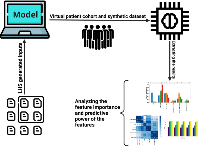
Our study started with the generation of a comprehensive list of 20,000 parameter sets (synthetic patients) utilizing the Latin Hypercube Sampling (LHS) method. These parameters were then integrated into our mathematical model to simulate the infiltration widths after the resection for 3 to 12 months. The data we obtained helped create a simulated dataset that mimics a group of patients. This dataset served as the basis for our subsequent analysis, implementing machine learning techniques to unravel the model’s predictive power and recognize the significance of various features within it (this cover has been designed using resources from Flaticon.com).

Full size image

We developed a model to address the key inquiries outlined in the introduction. Our model encompasses tumor cells, TAMs, and oxygen levels interlinked through a partial differential equations (PDEs) system. By analyzing the tumor’s behavior under the influence of TAMs and oxygen levels, we delved into understanding the dynamic interactions within the system. Initially, we evaluated the model’s performance against two clinically relevant observables: IW and TS, illuminating the system’s behavior dynamics. Next, employing global sensitivity analysis, we probed the parameters to discern their impact on IW and TS outputs. Finally, leveraging the model as an in silico platform, we conducted simulations on a virtual cohort of 20,000 patients to predict IW levels at 3 and 12 months post-resection. This rigorous analysis not only unveils the significance of localized biopsies but also provides insights into the predictive capabilities of individual parameters vis-à-vis target values.

The role of TAM and glioma cell interactions towards GBM growth and invasion

Increasing glioma oxygen consumption rates increase the infiltrative behavior of tumor cells

We initiated our analysis by scrutinizing the impact of oxygen consumption rate on a parameter space (D, b). In Fig. 3, we present a simulation map illustrating the IW across three distinct glioma oxygen consumption rates: h2 = [5.73 × 10⁻⁴, 7D15.73 × 10⁻³, 7D15.73 × 10⁻²]. Notably, simulations conducted under reduced oxygen consumption rates show a prevalence of tumors characterized by decreased proliferation yet elevated infiltration rates, indicative of a propensity for invasive behavior. Moderate oxygen consumption rates, conversely, correlate with a marginal uptick in tumor proliferation rates, while the inclination toward invasiveness remains conspicuous. It is discerned that in normoxic conditions, tumors tend towards nodular growth. However, escalating oxygen consumption rates correspond with a pronounced shift towards invasive behavior across tumors, irrespective of their intrinsic proliferation rates. This phenomenon is attributed to hypoxia-induced cellular migration, fostering a tumor infiltrative pattern. Figure 3 depicts the differential IW content in response to varying oxygen consumption rates, revealing subtle fluctuations in IW (II-I), in stark contrast to the pronounced disparities observed in IW (III-II). Precisely, a 1.96% increase in the maximum values of IW from IW I to IW II is noted, followed by a substantial 32.69% increase from IW II to IW III. This latter observation underscores the pivotal influence of hypoxia in driving the transition of highly proliferative glioma cells toward a more aggressive and infiltrative phenotype.

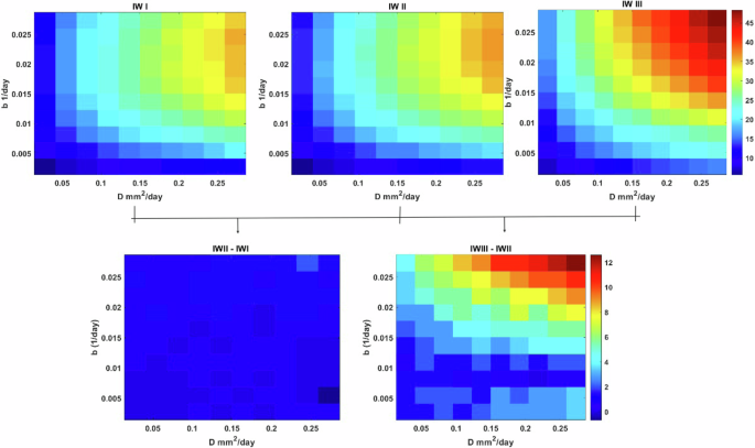
The maps are based on intrinsic proliferation and infiltration rates ((Din left[2.73times 1{0}^{-3}right.), 2.73 × 10⁻¹) and (bin left[2.73times 1{0}^{-4}right.), 2.73 × 10⁻²) A) IW for the maps for different values of glioma oxygen consumption rates (h2 = [5.73 × 10⁻⁴, 7D15.73 × 10⁻³, 7D15.73 × 10⁻²] and B) are the differences between IW I-II and IW III-II.

Full size image

Figure 4 illustrates that under low oxygen consumption rates, gliomas tend to grow and proliferate more than infiltrate. Remarkably, this pattern remains consistent even at moderate oxygen consumption rates. However, as the TME becomes increasingly hypoxic due to elevated oxygen consumption rates by glioma cells, a notable decrease in TS is attributed to a shift towards invasiveness and reduced proliferation. This shift becomes particularly evident when transitioning from TSI to TSIII. Quantitatively, the percentage decrease in TS is recorded as -0.42% from the maximum value of TS I to TS II, followed by a more substantial decline of -3.5% from the maximum value of TS II to TS III.

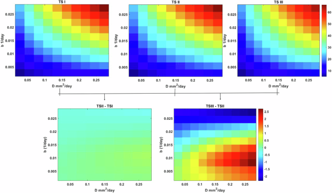
The maps are based on intrinsic infiltration and proliferation rates ((Din left[2.73times 1{0}^{-3}right.), 2.73 × 10⁻¹) and (bin left[2.73times 1{0}^{-4}right.), 2.73 × 10⁻²) A) TS for the maps for different values of glioma oxygen consumption rates (h2 = [5.73 × 10⁻⁴, 7D15.73 × 10⁻³, 7D15.73 × 10⁻²] and B) are the differences between TS (I-II) and TS (III-II).

Full size image

Time-dependent sensitivity analysis reveals the most effective parameter through the time to detection

Our time-dependent sensitivity analysis unveils the pivotal role of the diffusion rate of glioma cells D as the most influential parameter affecting both quantities of interest, namely IW and TS. Notably, the diffusion rate demonstrates a robust positive correlation with TS and IW outputs. This correlation arises from the capacity of glioma cells to extend outward into the tumor core, where they can support proliferation, thus fostering tumor growth and invasion. Similarly, the tumor proliferation rate b emerges as another dominant positive factor influencing both IW and TS outputs-this observation aligns with established understanding, highlighting the significance of these parameters in shaping tumor behavior. The glioma oxygen consumption rate parameter (h₂) emerges as a critical determinant, exhibiting a positive correlation with IW and TS. Variations in glioma consumption rate can modulate tumor invasiveness at higher values and promote proliferation at lower values, delineating normoxic and hypoxic regions over time. In addition to these key parameters, the phenotypic regulation term (t_n) exerts a notable positive effect on IW, particularly later, underscoring its role during the emergence of hypoxic tumor regions. Figure 5 visually presents the time-dependent sensitivity analysis for the 11 model parameters, offering a comprehensive insight into their dynamic impact on tumor behavior over time.

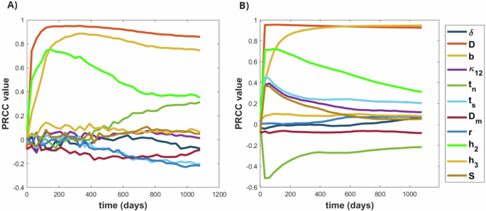
A The PRCC sensitivity analysis for the IW and B for the TS, depicting the time-dependent analysis of 11 parameters and 500 samples to see their effects on the output.

Full size image

The prognostic power of standard-of-care diagnostics and biopsy locus in predicting glioma recurrence

To address the question concerning the predictive potential of features within our study, we generated a synthetic dataset comprising 20,000 patient profiles. Primarily, this dataset undergoes meticulous preprocessing, laying the groundwork for an exhaustive analysis to calculate correlation coefficients and mutual information metrics for each feature. The latter quantifies even non-linear relationships among the variables. Following this, we partitioned the dataset into two primary categories: nodular and infiltrative gliomas. This stratification enabled us to assess the significance of specific features, such as macrophage ratios, Ki67 marker expressions, and tumor volumes as discerned in T1Gd-weighted and FLAIR imaging modalities ((T1-weighted imaging (T1) highlights anatomical structures with high contrast, providing precise detail on brain morphology. In contrast, FLAIR suppresses fluid signals, improving the visualization of lesions near fluid-filled spaces, which is particularly helpful for identifying peritumoral edema.). Through this comprehensive investigation, our objective is to determine the impact of these variables on the overall predictive accuracy of the dataset, evaluated through the mean squared error (MSE) metric.

Localized macrophages at the edge: superior predictors in Glioma Analysis based on Preprocessing the data

Our preliminary analysis of the raw complete dataset reveals insightful correlations between features and the target variable. In Fig. 6, the correlation coefficient heatmap illustrates the relationships among all features and the targets. Notably, tumor volumes at the time of detection demonstrate a strong correlation coefficient with the target, particularly with IW after 12 months post-resection. This positive correlation suggests that higher tumor volume values are a robust predictor for IW after resection, peaking at the 12-month mark. The mutual information plot in Fig. 7 reveals a strong correlation between these features, suggesting that initial tumor size may be a key predictor of the tumor’s behavior and size following recurrence. However, the behavior of the Ki67 marker presents an intriguing dynamic: negative values are observed for IW after 3 and 6 months, while a positive value emerges for IW after 12 months. This discrepancy suggests that in the early stages of tumor recurrence, a high Ki67 index might indicate rapid cell division, temporarily suppressing the tumor’s invasive characteristics as it focuses on rebuilding mass rather than invading new territories. As the tumor matures, its relationship with the microenvironment evolves, potentially fostering a more conducive environment for infiltration. Similarly, due to the highly non-linear behavior of the system, macrophages exhibit a similar pattern as Ki67. They have a very low negative effect on IW after 3 and 6 months and a positive value for IW after 12 months post-resection. This behavior can be attributed to the shift in macrophage phenotype, which is crucial for understanding their changing impact on tumor infiltrative behavior. Additionally, results highlight that macrophages close to the tumor resection threshold (edge region) exhibit higher values compared to macrophage ratios close to the tumor core (Fig. 6). This pattern is particularly evident for IW after 12 months post-resection, suggesting that macrophages predominantly harbor a pro-tumor phenotype and might be more beneficial at the edge to facilitate increased invasiveness.

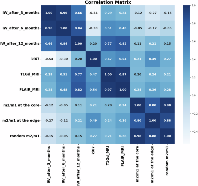
Correlation matrix heatmap for the raw dataset and the IW after 3, 6, and 12 months post-resection.

Full size image

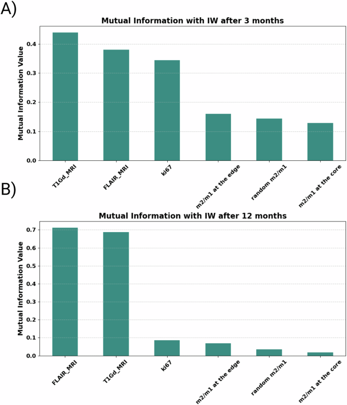
(A) 3 months and (B) 12 months after the resection. T1Gd and FLAIR MRI volumes have the highest correlation and mutual information values to the target.

Full size image

Impact of noise on infiltration width predictive models for nodular and infiltrative tumors

In this section, we evaluated the effects of noise on predictive modeling for nodular and infiltrative tumors at 3 and 12 months post-resection. Figures 8 and 9 present the performance metrics, including MSE and R², under various scenarios encompassing different feature sets.

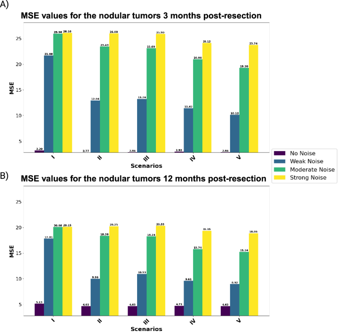
Each scenario represents a combination of biological and imaging markers to predict the output for (A) 3 and (B) 12 months post-resection.

Full size image

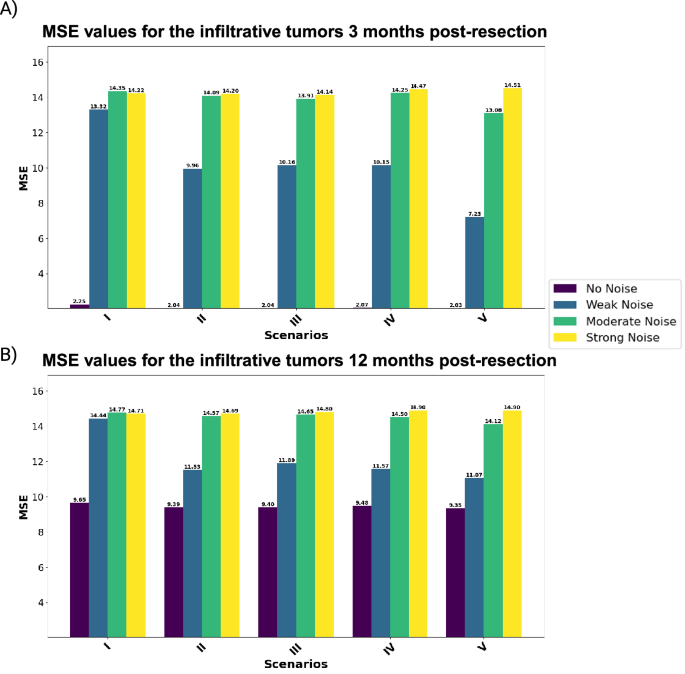
Each scenario represents a combination of biological and imaging markers to predict the output for (A) 3 and (B) 12 months post-resection.

Full size image

Analysis for nodular tumors: We begin with assessing the predictive performance of nodular tumors across different noise levels. Notably, zero-noise conditions consistently yield the best outcomes across all scenarios. For instance, the model achieves an MSE of 2.77 for nodular tumors three months post-resection. However, with the introduction of weak noise, performance deteriorates substantially, indicating a high sensitivity to noise. Incorporating macrophage ratios enhances model performance under noise-free conditions. A trend over the weak and moderate noise in both 3 and 12 months post-resection shows that localized macrophages perform better than random macrophages. This can easily be shown in Scenario V, which outperforms the other scenarios. On the other hand, increasing the noise to strong shows a very slight improvement in Scenario V compared to the other scenarios. Moving 12 months post-resection, the results show a higher MSE for the zero-noise cases compared to the dataset at 3 months post-resection. However, under weak noise, Scenario V demonstrates the most robustness (MSE: 10.12 and 8.92 for the values of 3 and 12 months after the resection, respectively). These results indicate the benefits of including both core and edge macrophage ratios, even though macrophages at the core are not good predictors compared to the ones at the edge.

Analysis for infiltrative tumors: Infiltrative tumors also show a high sensitivity to noise, with increased MSE under weak noise conditions. However, models with comprehensive features (Scenario V) display greater resilience against noise, particularly under weak noise levels. Despite the introduction of noise, Scenario V consistently yields the most accurate predictions, underscoring the importance of a broad feature set in enhancing model stability.

The comprehensive analysis highlights the significance of data quality in predictive accuracy, with nodular tumors showing greater vulnerability to noise compared to infiltrative tumors. Additionally, including macrophage ratios enhances predictive performance, particularly in scenarios with low to moderate noise conditions. For both kinds of tumors, the feature set consisting of Ki67, T1Gd, and FLAIR MRI, and macrophage ratios at the core and edge of tumors (Scenario V) offers the most accurate predictions.

Robustness of feature importance in predicting infiltration width post-resection

This section investigates the robustness of feature importance in predicting IW post-resection across different data quality levels. Figures 10 and 11 illustrate the feature importance for nodular and infiltrative datasets at both 3 and 12 months post-resection, considering varying noise levels. Initially, the Ki67 index emerges as a strong predictor in noise-free datasets, indicating its significance in tumor prognosis. However, the predictive reliability of Ki67 diminishes with the introduction of noise, highlighting its vulnerability to data perturbations. This observation underscores the heightened sensitivity of Ki67 to cellular proliferation rates, particularly in the early stages of tumor regrowth post-resection. This decline is likely attributed to the evolved state of the tumor at later stages, where the complexity of tumor biology extends beyond proliferation rates, rendering Ki67 a less definitive prognostic feature. Furthermore, macrophage ratios, particularly the m2/m1 ratio at the tumor edge, exhibit stability across different noise levels, suggesting intrinsic characteristics of the TME’s response to resection. This stability underscores the potential utility of localized biopsies in predicting tumor behavior, even in scenarios with poor data quality. On the other hand, under the no-noise scenario, non-localized biopsies perform better than localized ones. This can be due to the well-distributed data at the TME.

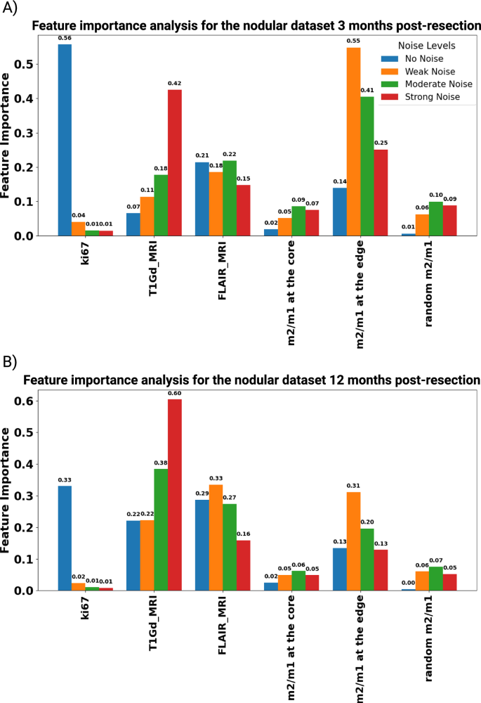
The bar chart shows feature importance scores for different features in a dataset under four conditions, No Noise, Weak Noise, Moderate Noise, and Strong Noise, for the nodular dataset at (A) 3 and (B) 12 months post-resection.

Full size image

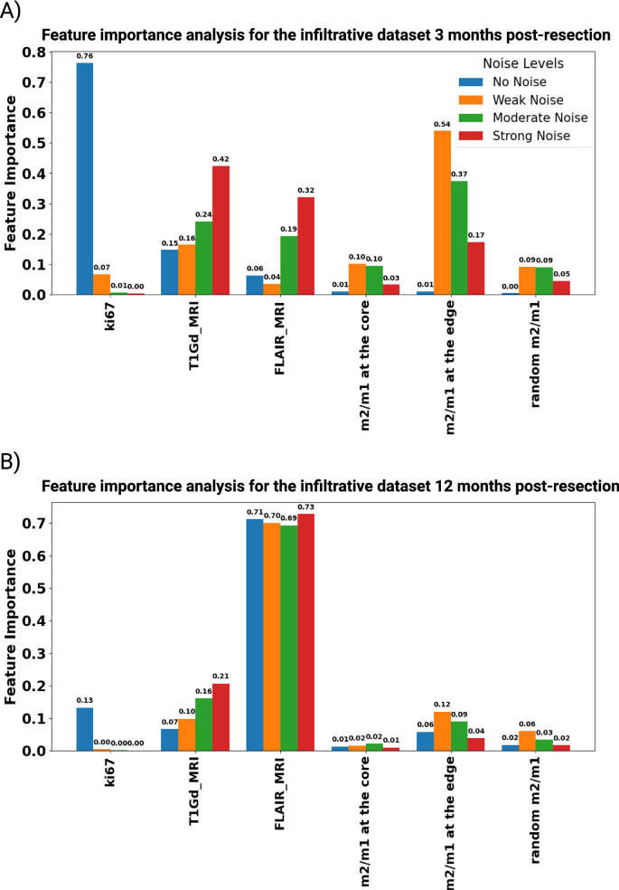
The bar chart shows feature importance scores for different features in a dataset under four conditions, No Noise, Weak Noise, Moderate Noise, and Strong Noise, for the infiltrative dataset at (A) 3 and (B) 12 months post-resection.

Full size image

Overall, the analysis highlights how crucial strong feature selection and careful data quality management are for improving the clarity and trustworthiness of predictive models in assessing tumor prognosis.

In this study, we developed a spatio-temporal mechanistic model that provides new insights into the dual phenotypic plasticity of glioma cells and macrophages and their intricate interactions. Our model includes the nonlinear dynamics of these interactions and reveals how macrophages and oxygen availability impact the phenotypic plasticity of glioma cells through mechanisms governed by the “go-or-grow” dichotomy. This idea, which describes the critical trade-off between tumor cell proliferation and migration, is captured effectively in our model, as reflected in the complex biological behaviors of GBM observed in clinical settings and experimental studies. The model shows that changes in oxygen consumption rate can lead to more infiltrative and less proliferative tumor phenotypes, which aligns with previous studies that explore the impact of microenvironmental factors such as oxygen availability and mechanical stress on tumor dynamics^37,38. After exploring the parameter space via global sensitivity analysis, we used the model as a virtual reality to investigate the predictive power of available in silico biopsies and MRIs toward recurrences after resection. To comprehensively assess the predictive capabilities of the features generated from our model, we constructed a synthetic dataset comprising 20,000 virtual patient profiles. This dataset undergoes preprocessing to ensure data integrity and usability, incorporating variability through applying Gaussian noise with three distinct standard deviations. We employed statistical techniques to derive correlation coefficients and mutual information metrics for each feature, then classify the dataset into nodular and infiltrative gliomas, representing two distinct patterns of brain tumor growth crucial for guiding clinical management and mathematical modeling. Our results indicate that at the early stages of intratumoral vessel density (IW) post-resection (IW after 3 months), Ki67 emerges as the strongest predictive biomarker for the zero-noise dataset, reflecting the role of proliferative tumor cells at the early stage of relapse. However, even weak noise significantly diminishes Ki67’s predictive power, highlighting the impact of technical and biological variability on biomarker assessment. Conversely, the m₂/m₁ ratio at the tumor edge exhibits high predictive power, especially for recurrence 3 months post-resection, suggesting the potential necessity of locus-specific biopsies in improving predictability. Interestingly, the latter is rather robust for weak to moderate noise levels. Our analysis also reveals that T1Gd and FLAIR MRI tumor volumes exhibit a stronger correlation with tumor recurrence at 12 months post-resection, indicating their enhanced predictive capacity for advanced, recurrent tumors compared to early-stage ones. This can be explained since tumor scans set the initial conditions for any predictive model. In particular, MRI-based measurements are pivotal in stratifying patients based on their risk of late recurrence, thereby informing more tailored post-surgical interventions and monitoring strategies. This can also indicate the important role of image analysis and radiomics data in predicting tumor prognosis. However, our study is limited by the inherent assumptions and simplifications required during the model development. The deterministic nature of our model might not fully account for the stochastic variations seen in actual biological systems despite introducing controlled noise to simulate this randomness. Additionally, we do not consider the impact of chemo- and radiotherapy on relapse, focusing instead on investigating the predictive power of generated features within a synthetic reality scenario. In our study, we focused simplistically on the role of monocyte-derived macrophages, which circulate in the blood vessels and are recruited by tumor cells. The potential particularities of resident microglia are not included in our model. Moreover, as hypoxia is acknowledged as a factor in our assumptions, we maintain a constant uniform value for the vasculature within the TME for simplification. In our imaging approach, we used synthetic classical MRI data, specifically FLAIR and T1Gd as the conventional MRI modalities. However, the MRI protocol could be expanded to include modalities such as PET, DTI, DWI, ADC, and SWI for each patient. These additional modalities could provide a richer dataset and enhance the information for patient cohort analysis. In summary, our study offers valuable insights into the predictive power of available features in predicting tumor recurrence post-resection in virtual reality and by providing a mathematical framework. Future studies, both in silico and experimental, could help validate and identify the predictive power of existing features, facilitating more personalized treatment strategies for glioma patients.

Mathematical modeling of the interactions between glioma and macrophages

In this study, macrophages are added to a system of PDE equations, playing an active role in interacting with glioma cells by inhibiting and activating glioma growth and infiltration. The basic model is developed previously by considering tumor vasculature and oxygen concentration^37,38. In this work, we assumed tumor vasculature as an implicit parameter that influences the influx of TAMs and oxygen transport, and for simplicity, we assume it as a constant value. Figure 12 shows a schematic of the model’s variable interactions and how macrophages impact the dynamics of gliomas with the main assumptions.

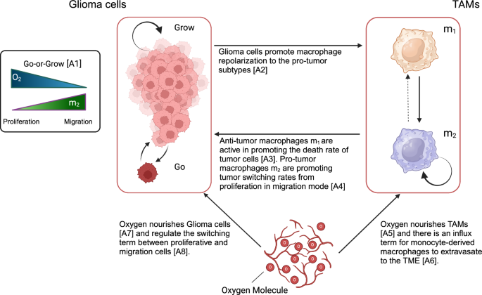
The scheme shows a holistic view of the interactions and switching terms for glioma and TAMs cells in the TME. (Created with BioRender.com).

Full size image

The variables are ρ_m(x, t) as the glioma infiltrative cells (Go), ρ_p(x, t) as the glioma proliferative cells (Grow), n(x, t) refer to the amount of oxygen as the nutrient factor, m₁(x, t) refer to the anti-tumor TAMs, and m₂(x, t) refers to the pro-tumor TAMs; where ((x,t)in {{mathbb{R}}}^{d}times {{mathbb{R}}}_{+}) and d is the dimension of the system.

The main assumptions are as follows:

1. A1

   Glioma cells are assumed to be two different phenotypes, namely proliferative or migratory (infiltrative) cells that depend on the TME stimulants and signals. High (low) oxygen availability and low (high) pro-tumor TAMs induce proliferative (migratory) phenotypes^{17,19,37,38,43,44}.

2. A2

   Glioma cells significantly influence the macrophage polarization in the TME employing key cytokines like IL-4/13 and TGF-β playing a pivotal role^30,45.

3. A3

   M1-like macrophages are characterized by features working against tumor progression, primarily due to their intrinsic capabilities of phagocytosis and the generation of enhanced anti-tumor inflammatory responses^46,47.

4. A4

   Pro-tumor (“M2-like”) TAMs tend to increase the tumor-invasive behavior. Therefore, we assume that M2-like macrophages are promoting the phenotypic switching rate from proliferation to the migratory glioma cells⁴⁴.

5. A5

   and A7 oxygen nourishes glioma and TAMs cells in the TME^48,49,50.

6. A6

   Monocyte-derived macrophages enter the CNS via the tumor vasculature²⁷.

7. A8

   Oxygen concentration plays a specific role in changing the glioma phenotypes. Under normoxic conditions, glioma cells maintain a certain phenotype optimized for growth and proliferation. However, in hypoxic conditions, where oxygen levels are reduced, glioma cells can switch to a more aggressive phenotype, often associated with increased invasion and resistance to treatment^48,49.

Glioma cell dynamics

We introduced the density of migrating and proliferating glioma cells, denoted by ρ_m and ρ_p, respectively. The switching term from proliferation to migration depends on the pro-tumor macrophages (m₂) and oxygen concentration (n). The equations for the two distinct glioma phenotypes are as follows:

In this part of our model, D (mm²day⁻¹) represents the infiltration rate, quantifying migratory glioma cells’ invasive behavior or how fast they are migrating to the brain tissue. The parameter δ (mm(cells.day)⁻¹ denotes the macrophage-induced death rate, indicating the rate at which pro-inflammatory macrophages (m₁) lead to the death of glioma cells. In the second equation for the proliferative glioma cells, b (day⁻¹) is the proliferation rate of glioma cells, determining how quickly these cells (ρ_p) multiply within the tumor microenvironment. The carrying capacity K (cells(mm)⁻¹) represents the maximum population density that the environment can sustain for the gliomas, limiting their growth based on available resources. Together, these parameters form the basis of the model and depict the “go-or-grow” dichotomy between the glioma cells. Moreover, f_mpρ_m and f_pmρ_p are the switching terms between the two cell phenotypes. The switching parameters (f_mp and f_pm) are depending on the oxygen concentration and M2-like macrophages.

The system can be reduced to a single equation with a density for both glioma cell phenotypes. This assumption appears reasonable, as intracellular mechanisms like signaling pathways that control the phenotypic transition function on significantly shorter time scales than those of cell migration and proliferation^37,38. Consequently, it is presumed that the switching of phenotypes occurs more rapidly than cell division and movement, enabling the expression of ρ_m and ρ_p concerning ρ. We can express a ρ = ρ_m + ρ_p and f_pmρ_p = f_mpρ_m as follows:

Thus, we can express the glioma density as follows:

α(m₂, n) and β(m₂, n) were defined as:

Therefore, we have a combined equation for the glioma cells with the effective infiltration and proliferation term based on the values of α(m₂, n) and β(m₂, n).

Glioma phenotypic switching term

As we briefly described in Fig. 12, glioma cells can change their phenotype into migration or proliferation due to the oxygen and effect of TAMs. Based on prior studies, we incorporated a linear function of oxygen into the phenotypic switching model^37,38. Whereas, we assumed m₂/K_m for the TAMs to represent the effect of pro-tumor macrophages on the glioma cells. TAMs release factors (IL-6, IL-1β, EGF, TGF-β, STI1, and PTN) that promote tumor progression³⁰. This assumption reflects the influence of the quantity of pro-tumor macrophages in the TME on the phenotypic behavior of glioma cells. The function can be tailored to fit experimental data or specific biological scenarios. In this sense, we define the switching term as below:

γ_n is the small regularization term for the possible transition when oxygen is zero. Figure 13 shows the 2D plot behavior of (alpha ({m}_{2},n)=frac{{f}_{pm}}{{f}_{mp}+{f}_{pm}}) and (beta ({m}_{2},n)=frac{{f}_{mp}}{{f}_{mp}+{f}_{pm}}) for the different values of m₂ and n.

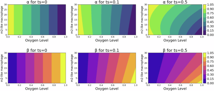
These plots reveal the dependency of switching terms, indicative of the migratory cell transition rate within the TME, on the interplay between environmental oxygen and the M2-like parameter, emphasizing the complexity of cellular behavior in response to the TME.

Full size image

Then, the transition terms for α(m₂, n) and β(m₂, n) become:

The terms α(m₂, n) and β(m₂, n) encapsulate the central role of oxygen and TAMs in the TME, influencing glioma plasticity and regulating diffusion and proliferation rates of glioma cells based on the availability of oxygen and TAMs. The nonlinearity of these terms arises from the division of linear components, resulting in a ratio that does not adhere to linearity concerning either variable. Consequently, α(m₂, n) and β(m₂, n) represent nonlinear functions of m₂ and n. We hypothesized that TAMs facilitate tumor infiltration, while oxygen levels simulate normoxic and hypoxic regions where the tumor tends to grow or infiltrate, respectively.

TAMs dynamics in the TME

To model the TAMs in the spatiotemporal domain, we simplified the known broad spectrum of macrophage polarization and simplistically assume two major populations: pro-inflammatory (m₁) and anti-inflammatory (m₂) TAMs. In this simplified concept, neglecting the pre-existent macrophage-like population of microglia, the m₁ macrophages have an influx based on the amount of tumor vasculature. We also added a diffusion term to incorporate the infiltration of TAMs in the TME. The presence and quantity of glioma cells enhance the phenotypic switching between pro-tumor and anti-tumor TAMs. Glioma cells release chemoattractant molecules (Periostin, SSP1, GM-CSF, SDF-1, ATP, GDNF, CX3CL1, LOX, HGF/SF, MCP-1, MCP-3, CSF-1, Versican, and IL-33)³⁰ that recruit and reprogram TAMs to facilitate their tumor progression. The equations for m₁ and m₂ are as follows:

where D_m is the diffusion term for macrophages and κ₁₂, κ₂₁ are the switching rates between two extreme macrophage phenotypes. K_p is the half-saturated rate of glioma cells for macrophage recruitment, and S is the recruitment coefficient, which is implicitly multiplied by the TAMs carrying capacity K_m. (H(n-{n}_{cr})=1-frac{1}{1+{e}^{-2theta (n-{n}_{cr})}}) is the logistic function that shows the effect of oxygen on the growth of pro-tumor TAMs.We use this logistic formulation to approximate a Heaviside function to smoothly model the oxygen concentration effect. This term models the hypoxic and normoxic regions of the TME, where pro-tumor macrophages infiltrate in hypoxic areas. The accumulation of TAMs in hypoxic zones within tumors is often linked to a negative outcome in clinical settings^35,36. These macrophages are drawn to these low-oxygen areas by following the trail of certain chemical attractants. Once there, TAMs contribute to tumor growth and progression through various mechanisms. They promote the formation of new blood and lymph vessels (angiogenesis and lymphangiogenesis), assist in the spread of tumor cells (metastasis), and suppress immune responses, thereby aiding the tumor’s survival and expansion^35,36,51.

Oxygen concentration dynamics

Oxygen is delivered to the brain tissue by the vascular network in the brain and by the functional blood vessels through the tumor bulk to be consumed by the cells such as gliomas and TAMs in the TME. The oxygen transport in the brain is conducted by diffusion and convection⁵². In this work, we only considered the diffusion form of oxygen transport throughout the TME. The functional vasculature delivers oxygen, and the supply rate is proportional to the difference between normal oxygen concentration in the brain n₀ and the TME.

where D_n is the oxygen diffusion coefficient, h₁ is the permeability coefficient of functional vasculature, v is the constant parameter for the vasculature, we assume a constant value that is uniform through the space, h₂ is the oxygen consumption range by the glioma cells, and h₃ is the TAMs oxygen consumption rate.

Model parameterisation

The values for parameters used in the model’s simulations are primarily sourced from existing literature. When specific data is unavailable, estimates are made to closely align with physiological conditions, guided by relevant physical and biological reasoning. In this case, we estimated the values for TAMs diffusion rates D_m, TAMs consumption rate h₃, and regularization terms t_s and t_n based on the closest relevant physiological conditions. For the sensitivity analysis, a wide range of values is chosen based on the interesting parameters to show their sensitivity and correlation to the observable outputs. Table 1 depicts the parameter values used in this study.

The full model

The governing equations, including a system of coupled partial differential equations which is used for the numerical simulation, are as follows:

where oxygen and TAM-dependent switching terms are given by Eqs (8)–(9). We assume an initial density followed by:

Where the m₁ and m₂ have zero density at the beginning of calculations. ρ₀ and n are the positive parameters, and the density of glioma cells is distributed in a segment of length x₀ in a sigmoidal form where b > 0 is a constant value. This is a well-established assumption since we do not know when the original cell started growing. Therefore, we initially assumed a specific number of tumors with a similar form. L > 0 is the length of a one-dimensional computational domain in L = 300mm which is discretized into a grid from 2.5 × 10⁻³ to 2.5 × 10⁻² in a total simulation of about three years with a time-step of 30 days. ρ(x, t_d) is the initial condition after the tumor resection, where λ is the resection threshold⁵³. To derive the exponential tail of a traveling wave solution of the model, we can neglect the non-linear term growth (ρ(x)/K < < 1)⁵³ and the role of m₁ macrophages for inhibiting the tumor growth rate. Therefore, we can obtain the value as (lambda exp (-sqrt{frac{b}{D}}x))^53,54.

Both grid network and time steps are selected properly to avoid numerical instability. Furthermore, we examine a standalone host tissue where all system dynamics are exclusively attributed to the interactions specified in Eqs. (16)–(19). This premise leads to implementing fixed boundary conditions that prevent any flux.

where T_f is the end of the simulation time, which in this study is three years. In the no-flux boundary condition, no cell leaves through the boundaries.

Stability analysis

In the supplementary material, we provide the linear stability analysis for the glioma-free steady states of the diffusion-free model in dependence on these parameters. We found two such states which are non-negative. The trivial steady state [ρ_p, ρ_m, m₁, m₂, n] = [0, 0, 0, 0, 1] is associated with the healthy brain state since no monocyte-derived macrophages exist. We found this to be an (unstable) saddle point with four negative and one close to zero (although positive) eigenvalue. For the special case of t_s + t_n = 1, we can also infer the stability of another glioma-free steady state that exists in the hypoxic region where H ≈ 1, and macrophages are present. This state is relevant in the case of a broken blood-brain barrier and eventually after tumor clearance. This state is stable only for a proliferation rate greater than a critical value b_crit, whose value depends on a non-trivial combination of the other parameters. This can be understood as a local tumor-free state where macrophages are sufficient to clear the tumor.

Model observable outputs

The model is used to produce two clinically relevant observables: tumor infiltration width (IW) and tumor size (TS). IW is defined as the difference of distances from the core where the density of tumor mass is 80% and 2%, which is also considered the tumor edge. TS is obtained by integrating the spatial profile of tumor density divided by its maximum value. These outputs represent the most critical parameters for estimating tumor malignancy and understanding the impact of various factors on them^{37,38,55,56,57}.

Machine learning analysis

To address Question 3 concerning the predictive power of derived features, we have designed a methodology that evaluates various data availability scenarios, mirroring the post-surgical IW.

Data preparation for generating clinical dataset

For generating the synthetic dataset, we adopt Latin Hypercube Sampling (LHS), the same strategy used in the sensitivity analysis of the preceding chapter but considering a uniform distribution for all the parameters. LHS is an effective approach for navigating the complex, multidimensional parameter spaces typical for mathematical biology models. It divides each parameter’s range into equal likelihood intervals and selects one sample from each, thus ensuring a broader distribution across the entire parameter space⁵⁸. This stratification method offers a more even coverage than simple random sampling from a uniform distribution, which often leads to sample clustering and inefficient space exploration. Utilizing LHS in creating the synthetic dataset results in a collection of parameter combinations that are more representative and varied, thereby enhancing the analysis of the model’s responses to different conditions.

In this section, we selected key parameters that differ across the established clinical spectrum and our hypothesis to create 20,000 synthetic patients. These parameters serve as inputs for the model, from which we derive the concentrations of glioma, TAMs, and oxygen at a randomly determined detection time. The detection time varies for each patient, reflecting the unpredictable timing of MRI diagnoses of the tumor from initial growth. Upon determining the detection time for each synthetic patient, we set the tumor density to zero and treated the remaining tumor mass as the starting point for the new post-surgery condition. Figure 14A illustrates the process of choosing the detection and prediction times and establishing the new baseline condition for each patient’s post-surgical profile. To compile the dataset, we simulated the acquisition of biopsies and MRI scans for patients. This method enables us to evaluate the predictive capacity of various features. We determine MRI data by utilizing 80% of the maximum tumor density for T1Gd-weighted images and 16% for FLAIR images, which helped us to estimate the tumor volume via these imaging techniques^56,57. These amounts for identifying the tumor volume for each of the MRI modalities are arbitrary and can be defined with various ranges of density detection. Additionally, we calculate the Ki67 biomarker, indicative of the patient-specific proliferation rate, using the formula proposed by Macklin et al.⁵⁹:

In this equation, PI represents the proliferation index, equated with the Ki67 values, and AI denotes the apoptotic index, for which we fixed a value of 0.831%. The apoptosis duration τ_A is assumed to be 8 hours, and the cell cycle time averages 25 hours, following the parameters provided by Macklin et al. and supported by additional sources^59,60. To collect the remaining biopsy data, which includes information on tumor cells and macrophages, we devise a strategy that segments the tumor from its core to its periphery into five distinct zones. We then select a random location within each zone to sample. At these chosen sites, we record the concentrations of tumor cells and macrophages. We obtained the average value for the macrophages at the tumor core and tumor edge based on these bins shown in Fig. 14E. We considered the values from the first two bins for the macrophages at the core and the last three bins for the macrophages at the edge (lower than 60% of tumor maximum glioma density). Meanwhile, for the non-localized biopsy, we assume a random location from the tumor core until the 16% of maximum glioma density. We chose five different random samples within this range and obtain the mean value of these random samples. Figure 14B visually represents the process, depicting the biopsy samples extracted across the tumor’s profile. In the end, for the more realistic scenarios, we implement three different amounts of Gaussian noise with multiple standard deviations (Std = 1, 5, 10) to make the biopsy data noisy. This procedure allows us to investigate biopsy data’s predictive power and quality in different situations. Figure 14C shows the visualized noises, which include weak, moderate, and strong noise based on the standard deviation.

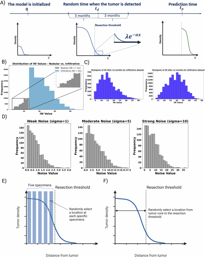
A Initially, the model begins at t = 0, simulating tumor density, oxygen levels, and macrophage activity. For each simulated patient, a detection time is randomly assigned within a range of ± 3 months. Once the detection time for a patient is established, a hypothetical surgical resection is performed based on a predefined resection threshold. This process involves removing the resected area, leaving behind a truncated profile of tumor cells. These remaining cells are then considered the new starting point for further simulation, which continues until achieving our objective of generating clinically relevant observable IW for 3, 6, and 12 months post-resection. In this schematic figure, B we divided the cohort into two subgroups, Nodular and Infiltrative, based on the IW at detection time. This category allows us to investigate the predictive power of values across the range of formless aggressive to massively infiltrative tumors. C The sample of histograms for the IW post-resection after 3 and 12 months for the infiltrative cohort. IWs are our target values for the prediction. E We selected five virtual “specimens”, representing either biopsies or portions from the resected tumor, at the time of primary diagnosis. Then, we extract the data, including tumor cell and macrophage densities, from these five simulated “specimens.” F We selected random locations representing the full range from the tumor core to the resection margin.

Full size image

Evaluating predictive models for infiltration width in glioma subtypes

Understanding the difference between nodular and infiltrative gliomas is crucial for modeling tumor growth and response to therapies. Our approach begins with categorizing the dataset into two distinct tumor subgroups: nodular and infiltrative (Fig. 14E). This classification is based on the IW value observed during tumor detection for each patient (Fig. 14F). Specifically, we designate tumors falling within the first quartile of IW values as nodular, while those exceeding this threshold are classified as infiltrative. Following this categorization, we conduct rigorous analysis to identify the most effective regression model for predicting IW at two critical post-resection intervals: 3 and 12 months. This selection process is informed by assessing the significance of various features within our dataset. Our methodology also incorporates two distinct biopsy techniques: localized and non-localized. This means we take the values from the tumor core and the edge for the localized biopsy and randomly pick values from the range spanning the tumor core to the detection threshold for the non-localized biopsy. Moreover, we analyze the predictive power of each feature based on the metric values of MSE for the different case scenarios. Five case scenarios are introduced to predict the IW after 3 and 12 months. The scenarios are as follows:

1. I.

   [Ki67, T1Gd MRI, FLAIR MRI]

2. II.

   [Ki67, T1Gd MRI, FLAIR MRI, random m2/m1]

3. III.

   [Ki67, T1Gd MRI, FLAIR MRI, m2/m1 at the core]

4. IV.

   [Ki67, T1Gd MRI, FLAIR MRI, m2/m1 at the edge]

5. V.

   [Ki67, T1Gd MRI, FLAIR MRI, m2/m1 at the core, m2/m1 at the edge]

where “random m₂/m₁” refers to the non-localized biopsy, whereas “m₂/m₁ at the core” and “m₂/m₁ at the edge” refer to the biopsies from the tumor core and the closest region to the resection threshold. These scenarios depict the role of each feature, especially the role of m₂ to m₁ ratio for the localized and non-localized values. Figure 15 shows the flowchart, which depicts the holistic approach of this study. This procedure allows us to not only develop a mechanistic model, but it can also be used as an in silico base to study the effect of each feature on the recurrence after the resection in virtual reality.

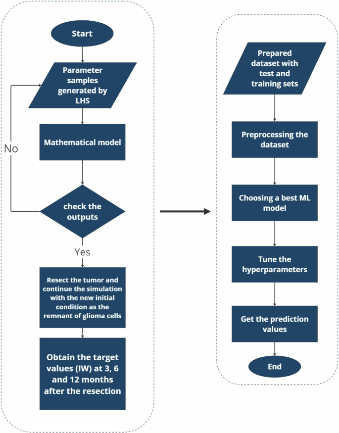
First, a mathematical model simulates tumor dynamics based on parameters generated via Latin Hypercube Sampling (LHS) and post-surgical conditions; second, the simulated data informs a machine learning pipeline for the prediction of tumor progression at future time points to explore the predictive power of features.

Full size image