Calibrated confidence learning for large-scale real-time crash and severity prediction

The global status report on road safety outlined that each year 1.35 million people die from road traffic crashes, and an additional 20–50 million people suffer from non-fatal injuries with incurring disability¹. Apart from these large deaths and injuries, road traffic injuries put a huge socio-economic toll² and cost the world economy US$1.8 trillion, which is equivalent to an annual tax of 0.12% on the global gross domestic product³. United Nations General Assembly set the target to bring the road traffic deaths and injuries to half by 2030⁴. Federal Highway Administration (FHWA) exert utmost efforts to minimize the deaths on roads⁵ to enhance road safety and improve transportation sustainability. To achieve this sustainability goal, a greater transition in transportation safety research is shifting from a reactive safety approach, analyses and modeling using data collected after the crash occurrence, to a proactive approach, analyses and modeling using real-time information before the crash occurrence^6,7,8. Researchers are contributing through their novel research and innovative methodologies to improve safety on roads⁹. This provides great leverage to predict and prevent crashes before they occur, and researchers have reached an advanced level in developing real-time crash likelihood prediction model with higher accuracy and lower false alarm rate (FAR)^{10,11,12,13,14,15,16,17,18,19,20,21}. However, there are some concerns regarding these real-time crash likelihood prediction models. First, the current state-of-the-art focused on improving accuracy only without paying proper attention to reducing computational expense, overcomplexity, and the large size of the proposed models. Particularly the state of the art has paid less attention to developing real-time crash likelihood and crash severity prediction models as a continuous process, where the crash events will be predicted first from real-world crash and non-crash scenarios, and then that framework will simultaneously predict the crash severity, i.e., fatal crashes, severe crashes, minor injury crashes, and property damage crashes (PDO) crashes. This study is an effort to address these limitations by proposing an effective calibrated confidence learning-based approach for real-time crash likelihood and crash severity prediction. Also, deployment strategies of our proposed approach in real-world situations will be discussed.

Our spatial ensemble learning blends ensemble learning and model generalization, like knowledge distillation, to enhance spatially heterogenous crash and severity prediction. Ensemble learning is commonly recognized as the process of combining the predictive outcomes from a set of machine learning models, like Bayes classifiers or deep neural networks, by applying different aggregation rules²². In real-time transportation safety applications, we employed an ensemble model that proves effective in addressing the heterogeneity challenge. By employing spatial divide-and-conquer modeling, our ensemble model produces an accurate solution with minimal false alarms. This approach can result in a sustainable solution that optimizes resource allocation efficiently. However, it may become cumbersome and computationally expensive²³, leading to an increase in carbon footprint and impacting overall sustainability. To tackle this issue, we reduce model size and optimize training pipeline for efficient training, which not only reduced training cost but also has the potential to minimize energy consumption associated with model training. Also, another issue arises where the constituent model may experience local optima due to localized training, and thus, model generalization becomes critical. We investigated several regularization methods to alleviate this issue. In particular, we examined knowledge distillation for performance improvement. Among existing research, the knowledge distillation technique is commonly used for model compression by distilling the knowledge from a larger deep neural network (aka teacher model) into a small network (aka student model)^24,25,26. Latest research found that this method can regularize the model to avoid overfitting, thus improving generalization performance²⁷. Therefore, in our investigation, we also explored this technique to enhance real-time crash and severity accuracy for more reliable training that minimizes false alarms. This approach aligns with our commitment to providing a sustainable transportation safety solution that efficiently allocates resources for preventive measures, thereby mitigating the economic costs associated with crash intervention.

More specifically, our study investigated extensively big data with readily available real-time variables collected from Interstate-75 (I-75) freeway; developed individual segment-level models for crash likelihood prediction and crash severity prediction. These individual segment-level models are spatially ensembled to improve performance. To save training costs, each segment-level model is a lightweight multilayer perceptron. The training of all these lightweight models conserves hundreds of hours compared to the extensive training of one large model on all data across various segments. This accomplishment leads to significant reductions in carbon footprints, contributing to environmental conservation. Next, we distilled knowledge from the ensembled models to improve model generalization for higher accuracy and lower false alarms. We examined the viability of the developed models in identifying specific crash types, i.e., rear-end crashes, sideswipe/angle crashes. Last but not least, we delved into the impact of this approach on traffic safety planning, outlined the deployment strategy for real-time practice, and discussed the inference time efficiency of this solution. In particular, our approach can operate effectively over an extended period after a single training. This extended operational efficiency contributes to another notable reduction in the carbon footprint associated with frequent retraining, particularly when viewed from a long-term perspective. In sum, spatial ensemble leveraging can lead to energy-efficient model training. Such sustainable transportation modeling methodology is completely novel and has substantial potential to contribute to real-time transportation safety.

For an extensive review of the earlier literature related to real-time crash and severity, the study explored different databases including Institute of Electrical and Electronics Engineers (IEEE) Xplore digital library, Accident Analysis & Prevention, Transportation Research Part C: Emerging Technologies, ASCE Library, Scientific Reports—Nature, Google Scholar, Transportation Research Part B: Methodological, ScienceDirect, Transportation Research Record: Journal of the Transportation Research Board, Web of Science, Scopus, and ACM Digital Library. Relevance of the articles related to the current study was assessed based on a rigorous investigation of the methodology, data, modeling technique, results and discussions, contributions stated in the studies, and finally, methodologies and findings from the selected journal articles on real-time crash and severity are presented and discussed.

Extensive review of the literature revealed that most studies in real-time transportation safety focused on real-time crash likelihood prediction. Particularly proposing a new modeling technique for real-time crash likelihood prediction was the main focus of those studies^13,28,29. To enhance the accuracy of the proposed technique, efforts were also made to address the data imbalance issue of crash and non-crash data^30,31, investigate the most contributing factors in developing real-time crash likelihood prediction model^32,33,34, focus on developing a model for a particular section of a roadway^19,35,36 or develop models based on traffic state³⁷, optimize the prediction performance in different levels, i.e., output level, data level and algorithm level³⁸. Some efforts to assess the viability of spatial and temporal transferability of real-time crash likelihood prediction models³⁰ or propose a workflow for real-time crash likelihood prediction, quantification, and classification³⁹ were also found. Real-time crash severity-related studies have evolved in the literature since 2010, and these studies are conducted in the USA^{11,40,41,42,43,44,45,46,47,48,49}, China^50,51, France⁵², Greece⁵³, and Iran⁵⁴. Most of these studies are conducted on Freeways/Expressways/Toll Roads. Some of them also considered using data collected from arterials^48,49,53. The length of the roadway section considered in those studies ranged from very low, i.e., 7.7 miles⁴⁹, to sufficiently large, i.e., 111 miles⁴⁷. The real-time data study period used for modeling or analyses in those studies ranged from 1 year^40,43,46 to 5 years^53,54. Here we explored all studies relevant to real-time crash severity predictions or analyses, although there is less effort found to develop models for real-time crash severity prediction.

Mainly four data sources, i.e., crash data, traffic data, weather data and road geometric data, are used in those studies. Some studies also used events data^48,49, signal timing data^48,49, and land use characteristics data⁵⁴. Crash data were collected from police crash reports⁴¹, government organizations, i.e., different departments of transportation (DOTs)⁴², and private entities, i.e., signal four analytics (S4A)⁴⁸. Traffic data were collected mainly from loop detectors⁵², automatic vehicle identification (AVI)⁴⁴, regional integrated transportation information system (RITIS)⁴⁷, automated traffic signal performance measure (ATSPM)⁴⁸, Camera⁵⁴, and microwave vehicle detection system (MVDS)⁴⁰. Most of these traffic data sources update traffic information, i.e., speed, volume and lane occupancy, in every 30 s⁴³. However, ATSPM used in some studies was found to update traffic information more frequently and it was in every 0.10 s⁴⁹. Weather data was collected from the closest weather stations of the roads considered, and roadway geometric data was obtained from the Roadway Characteristics Inventory (RCI) provided by the DOTs⁴⁴ or organizations⁵⁰. Events data and signal timing data were obtained from ATSPM^48,49, and land use characteristics data was obtained using open street map (OSM)⁵⁴.

After initial data collection, traffic data are generally aggregated to generate more useful variables for modeling or analyses, i.e., average, standard deviation (SD), and coefficient of variation (CoV). Most of these crash and severity-related studies aggregated the raw traffic information into 5 min. However, some studies aggregated it to 6⁴⁴, 10⁴⁷, 15 min⁴⁹, and 1 h⁵³. Some studies also aggregated the weather data in a similar fashion like traffic data to 1 h^41,42. Then aggregated real-time traffic and weather information are matched with crash and road geometric information. It is a common practice in real-time transportation safety research to use 5–10 min prior traffic information to develop prediction models and most of the real-time crash and severity-related studies used 5–10 min prior traffic information of a crash occurrence⁴³. However, many studies considered real-time crash severity prediction as a more sophisticated task, and hence, they used 12–18⁵², 15 min⁴⁸, and 1 h^41,42 prior traffic and weather information to predict crash severity or analyze various aspects of crash severity prediction. Another notable observation is that most of these studies modeled or analyzed crash severity as a separate entity rather than a continuous process of predicting crashes first among crash and non-crash samples, and hence they only used crash samples^41,42,52. However, some of these studies considered both crash and non-crash samples in their initial dataset^43,45,53. They used different strategies to address the data imbalance issue of crash and non-crash samples. Some of the studies adopted a random selection approach of non-crash, and they used 1:20⁴³, 1:10⁴⁵ ratio of crash and non-crash samples. A few studies also used matched case-control to select non-crash samples, and they used a 1:2 ratio⁵³ of crash and non-crash samples. Some studies also used the Synthetic Minority Over-sampling (SMOTE) technique to address crash and non-crash data imbalance issues⁴⁰. Then, a dataset is prepared by integrating crash, traffic, weather, road geometric, and other data sources, and further cleaning and processing actions are performed to remove unrealistic and missing values. Some studies directly used this processed dataset for final analyses and modeling; some checked the multicollinearity issue by using Pearson’s correlation coefficient test/correlation matrix and dropped highly correlated variables^11,41; some applied important variable selection procedures, i.e., random forest, eXtreme Gradient Boosting (XGBoost), and used only the most significant ones^45,48.

Most of these studies on real-time crash severity prediction and analyses considered two levels or three levels of severity and used different combinations of the KABCO crash severity scale in combining these severity levels. In the original KABCO crash severity scale, there are five levels to define the severity of a crash, K refers to a fatal crash, A refers to an incapacitating injury, B refers to a non-incapacitating injury, C refers to possible injury, and O refers to property damage only^55,56. The studies considered two levels of severity, mostly defining their levels as injury crashes (combining K crashes, A crashes, B crashes, and C crashes) and non-injury crashes (O crashes or property damage only (PDO) crashes)^{11,44,45,46,49,52}. Some of these studies did not consider PDO crashes and categorized the severity levels into fatal-severe injury and slight injury^53,54. Some defined the two levels by grouping fatal or severe into one level and minor or no injury into another level⁴⁷. The studies used three levels of crash severity combining KABCO levels differently. Some used KA, BC, and O combination^41,43,51,52, whereas some used KAB, C and O combination⁴². Some studies did not follow any global crash-severity scale, rather, they followed their database-provided scale⁵⁰ or proposed new crash-severity levels based on the crash severity likelihood estimated based on traffic state and traffic-flow diagram⁴⁰. Such studies used three levels of crash-severity, i.e., High/Severe, Medium and low/light.

The majority of the real-time crash and severity-related studies focused on identifying the most contributing factors that lead to different levels of severity. Some studies assessed the special effects of some specific contributing factors on different levels of severity or developing a severity prediction model. For example, some studies assessed the impacts of real-time weather conditions on crashes and severity using real-time weather data^50,51. Few studies got more into it and investigated the rainfall effects on the severities of single vehicle and multi-vehicle crashes^41,42. Some studies investigated the effects of speed, traffic volume, and signal timing on different injury levels^49,52. Some studies identified the traffic conditions prone to injury and PDO crashes in different traffic states⁴⁵. Another study introduced camera spacing scenarios from the crash locations and measured their effect on the real-time crash severity model. This study concluded that camera spacing has a substantial impact on the significance of variables rather than the performance of models⁵⁴. However, very few studies actually developed or proposed a real-time crash and severity prediction model. One study developed a model to predict the crash likelihood at different levels of severity with a particular focus on severe crashes⁴³. Another study developed a predictive model for vehicle occupant injury in arterials using real-time data⁴⁸. Another study proposed a modeling technique to better capture the spatial correlation⁵¹. There was no study found that considered a real-time scenario, where both crashes were predicted first from the crash and non-crash events, and then the severity of the predicted crashes were further predicted. Only one study attempted to conduct such study⁴⁰, and they predicted the crashes first from crash and non-crash events. Then they clustered the predicted crashes into three severity levels based on the assumption drawn from the fundamental traffic-flow diagram. They did not predict the severity, rather, they clustered the severity following a non-conventional scale.

Overall, these real-time crash and severity-related studies contributed to the state of the art by providing some useful findings based on their research. Particularly higher traffic volume consistently reduced the likelihood of severe crashes⁵². Speed and other traffic flow characteristics were found to have differential effects on severity depending on the flow conditions and severity levels^43,52. For example, PDO crashes were found to occur at congested traffic states with fluctuating speeds and frequent lane changes, and KA and BC crashes were found to occur at less congested traffic flow conditions^43,44. Adjacent lanes having higher speed fluctuations tend to result in severe crashes⁴³. Another study specified this and concluded that differences in detector occupancy between adjacent lanes contribute significantly to PDO and injury crashes, speed differences between adjacent lanes and between upstream and downstream segments contribute to injury crashes, mean and standard deviation of speed are crucial for identifying high-speed state crashes⁴⁵. Angle, fixed object or run-off-road crashes were found to be more severe than rear-end crashes, and rear-end crashes were more likely to be severe than sideswipe crashes^48,50,53. Driving action is highly affected during rainfall conditions, and there is a high likelihood of severe crashes during rainfall⁴². Severe crashes are more likely to occur at segments with small horizontal curve radii and steep gradients during snow seasons and bad visibility conditions^11,44,50. Some studies recommended considering temporal heterogeneity, spatial correlations, and dependence between spatial correlations on different injury levels⁴⁶. However, one observation during this review is that some of these studies used many variables that are not available and deployable in real-time. For example, road user characteristics, vehicle characteristics, alcohol involvement, lighting condition, distraction-related factors, and number of vehicles involved^47,49,52.

Most of the real-time crash and severity prediction and analysis studies used statistical methods to perform their analyses and modeling. Ordinal logistic regression⁴¹, sequential logistic regression⁴¹, random parameters ordered probit model⁵², binary probit models⁴⁴, fixed-parameter logit model¹¹, random parameter logit model¹¹, genetic programming⁴⁵, finite mixture logistic regression⁵³, mixed-effects logistic regression⁵³, Bayesian multivariate space–time model⁴⁶, binary probit model with Dirichlet random effect⁴⁷, Bayesian spatial generalized ordered logit model⁵⁰, multinomial logit model⁵¹, spatial multinomial logit model⁵¹ are the statistical techniques those were used in the earlier studies. Few studies also used different machine learning techniques, i.e., support vector machine¹¹, extreme gradient boosting (xgboost)⁴⁸, random forest⁴⁸, classification and regression tree⁵⁴, artificial neural network⁴⁰, k-nearest neighbors⁴⁰, decision tree⁴⁰, naive Bayes⁴⁰, gradient boosting⁴⁰, convolutional neural network⁴⁰, and k-means clustering⁴⁰ were used by real-time crash and severity-related studies. Backward sequential logistic regression model^41,42, Bayesian binary probit model⁴⁴, random parameter logit model¹¹, XGBoost⁴⁸, spatial multinomial logit model⁵¹, and k-means clustering⁴⁰ were the recommended techniques among all these techniques.

Recommended models were selected based on some performance measures. Most of the superior models were selected based on the value of deviance information criteria (DIC)⁴⁶, Bayesian credible interval (BCI)⁴⁷, widely available information criterion (WAIC)⁴⁹, area under the receiver operating characteristic curve (AUC)⁴⁸, accuracy^41,52, sensitivity^41,52, specificity^41,52 and false alarm rate (FAR)⁴³. Table 1 presents the data analyses and modeling techniques of the earlier literature. In addition, the existing approaches in the earlier studies and their results are reported in Table 1.

This work attempted to solve these challenges by integrating ensemble modeling and model calibration. From the comprehensive literature review, only a few studies were found to apply an ensemble learning technique in only real-time crash likelihood prediction. These studies improved real-time crash likelihood model performance by applying ensemble learning. They fused outputs from two models using sum rule⁵⁷ and combined the output from a primary crash prediction model and a secondary crash prediction model to predict real-time secondary crash likelihood⁵⁸. To the best of our knowledge, no existing work, as shown in Table 1, has leveraged ensemble learning to address spatial heterogeneity modeling on crash severity prediction. Moreover, the arising difficulties, like model regularization, from spatial ensemble learning have not been investigated either. This study filled these research gaps, developed an effective approach, and examined the contributing factors. These important endeavors aim to harness spatial heterogeneity and deep learning to provide a sustainable transport planning solution. The efficiency extends to safety planning, resource allocation, and reduction of carbon footprint associated with model training.

The major contributions of our current work are summarized as follows. First, we leveraged our preliminary work on a generic non-IID crash prediction approach—spatial ensemble learning, to equip large-scale heterogeneous real-time crash severity prediction. To the best of our knowledge, it is the first work to leverage deep learning to conduct heterogeneity modeling for crash severity prediction. Second, we enhanced the proposed real-time crash prediction model by local model regularization for reliable likelihood prediction during training. This study is the first work to reveal the local optima problems for data-driven heterogeneity modeling, and we investigated different solutions to alleviate this problem for crash and severity modeling. Third, we further calibrated the model outputs in a post-calibration manner and leveraged the crash prediction model outputs to directly predict crash severity. This process improves crash feature recognition to enhance severity modeling. Moreover, this is the first work addressing real-time crash severity prediction with consideration of four levels of severity, to the best of our knowledge. Furthermore, we analyzed the contributing factors of the proposed method and revealed important features for effective severity modeling. Finally, we discussed the potential impact of the proposed approach on the real-world real-time traffic safety system implementation, including safety improvement, deployment framework, and deployment efficiency.

Preliminary: spatial ensemble learning

Observation data for developing real-time crash and severity framework are not independent and identically distributed (non-IID) due to their spatial heterogeneity. Particularly, the non-IID issue poses threats in two layers for the real-time crash and severity prediction framework. First, we need to predict crash likelihood using the non-IID crash and non-crash data collected from different segments with different geometric and traffic flow characteristics. Second, as the current study is considering four levels of crash severity, the non-IID issue also exists in this case for spatial heterogeneity and different proportions of K crashes, A crashes, BC crashes, and PDO crashes. To tackle this real-world challenge, we propose spatial ensemble learning to alleviate spatial heterogeneity and improve crash prediction accuracy.

First, separate zonal expert models were trained with local and IID data obtained from each individual homogeneous segment. These local and IID data were obtained by analyzing and clustering the crash and non-crash data for each individual segment. Then the developed zonal expert models were aggregated by importance weighting. This process is illustrated in Fig. 1.

Illustration of spatial ensemble learning technique⁵⁹.

Full size image

Equation (1) formulates the generic ensemble modeling process. To obtain the inference result ({P}_{i}left(y|{theta }_{i},x,Dright)) for label y from each deep neural network ({theta }_{i}), x is the selected feature x and D is the input. Then the final prediction (P(y|widetilde{theta },x,D)) is obtained by aggregating ensemble learning. This aggregation was performed using the weighted sum rule to leverage geospatial information.

Here, ({w}_{i}) is the importance weight of ({theta }_{i}) for final decision aggregation. ({w}_{i}) can be scaled to a probability with the convex combination. When there is no prior knowledge about the expertise of expert models, ({w}_{i}) is set to the same value of 1/N for all models.

The current study developed spatial ensemble learning based upon generic ensemble learning as illustrated in Fig. 2. First, the entire heterogeneous non-IID training data was separated into a set of zones where the subset of data exhibited near-IID patterns. Then machine learning was carried out to achieve zonal expert models as constituent models for ensemble aggregation using these near-IID zonal data. This aggregation process was based on importance weighting. Zonal expert model with modeling zone closer to data was put higher weight, and this is formulated in Eq. (2).

Here, z is the segment, ({D}_{{{rm {pred}}}}) is the datapoint for prediction and ({w}_{z}({D}_{{{rm {pred}}}}|{theta }_{z})) is the importance weight that depends on the spatial relationship between ({D}_{{{rm {pred}}}}) and modeling zone of ({theta }_{z})⁵⁹. The importance weight is estimated with the 2D Gaussian kernel function, where a higher probability is obtained within a shorter Euclidean distance. When prior knowledge is more accurate, the shape of the kernel will be narrower and sharper and approaches to Dirac delta function.

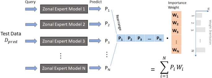
Weighted sum is conducted to aggregate ensemble prediction P given the D_pred and importance weight W.

Full size image

Confidence calibration

Regularization is an important technique by calibrating model outputs over training to alleviate overfitting, a typical machine learning problem, thus improving model generalization⁶⁰. Since overfitting on training data is reflected by abnormally high likelihood output, i.e. over-confidence on training samples, which causes incorrect likelihood for prediction, regularization attempts to correct the confidence by adjusting the model output likelihoods during the model training. For our severity modeling, because spatial ensemble modeling was adopted, a local model with fewer training data can encounter overfitting and over-confidence on training samples. Thus, we adopted regularization to calibrate the model confidence, i.e. model likelihood output, to achieve reliable model prediction and accurate severity modeling. In particular, our severity rating also leverages this confidence information into the decision process with post-calibration, which will be discussed in the next section. We investigated three important regularization techniques, including weight decay, label smoothing, and knowledge distillation^24,27,61,62.

Weight decay, usually also known as L2 regularization, is a common technique in machine learning, especially neural network training to reduce overfitting and improve model generalization⁶³. The weight decay regularization can be formulated as Eq. (3) given a regression problem.

where ({y}_{i}) is the true label, ({x}_{i}) is input feature data, ({h}_{theta }) is a model-like neural network, ({{boldsymbol{theta }}}_{{boldsymbol{i}}}) is model parameter and ({boldsymbol{lambda }}) is regularization magnitude. ({boldsymbol{lambda }}mathop{sum }nolimits_{{boldsymbol{i}}{boldsymbol{=}}{boldsymbol{1}}}^{{boldsymbol{n}}}{{boldsymbol{theta }}}_{{boldsymbol{i}}}^{{boldsymbol{2}}}) is regularization term. Lager ({boldsymbol{lambda }}) implies higher regularization.

Label smoothing is another commonly used regularization technique in machine learning, particularly neural network training⁶⁴. It aims to alleviate overfitting risk from the perspective of data labeling in training set. The main idea is to change labeling from 0/1 hard encoding to smoothed probability encoding like 0.1/0.9, etc. This smoothing process renders the labeling closer to decision-making since it is rare to predict a scenario with 100% or 0% likelihood. Accordingly, the technique enables robust training, better model generalization to unseen data, and reliable prediction confidence. The smooth labeling can be formulated as Eq. (4). Our problem is a binary classification, so L = 2. For the regression problem, we reduce ({bf{J}}) by zero.

where (alpha) is the smoothing ratio for the true class, L is the number of classes, (frac{alpha }{{boldsymbol{L}}{boldsymbol{-}}{boldsymbol{1}}}) is the distribution factor for the rest false classes, ({bf{I}}) is the one hot encoding vector for the true class, and ({bf{J}}) is the one hot encoding vector for the rest false classes.

Knowledge distillation, initially proposed for efficient prediction^24,27,65, is increasingly adopted to regularize the model for stronger generalization to the general data²⁷. Figure 3 shows the mechanism of knowledge distillation, where the outputs of the student network imitated those of the teacher network through optimizing knowledge distillation loss. The distillation loss is formulated in Eq. (5).

where (x) is the input data, (y) is the ground-truth label, L is the total loss consisting of distillation loss ({L}_{{{rm {dis}}}}) and mean-squared-error regression loss ({L}_{{{rm {mse}}}}), ({N}_{{rm {s}}}) denotes a distilled student network, ({N}_{{rm {t}}}) is a large teacher network, and (alpha) is the weight hyperparameter to balance two losses. Such distillation learning has the potential to reduce the size of the model, regularize zonal expert models, lower the FAR, and improve model generalization.

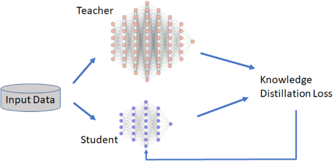
Student network is optimized with the output from the teacher model overall input data through distillation loss.

Full size image

Global severity post-calibration

Post-model calibration plays a crucial role in the deployment of models. It aims to enhance model’s ability to make accurate predictions on real-world, unseen data. Even modern neural networks require calibration after their initial training^66,67. The main objective of this calibration is to fine-tune the model’s output by adjusting the confidence levels associated with its predictions to ensure reliability. For example, neural networks can provide a probability distribution as output before making a classification decision. This probability serves as a measure of confidence, offering a more detailed insight into the inference analysis⁶⁶. In the context of predicting crashes, this confidence can be used to assess crash severity, as higher confidence indicates a higher likelihood of a severe crash.

We leverage this confidence information to map crash severity onto different confidence intervals: the more likely a crash, the higher the predicted severity. To achieve this, we incorporate temperature scaling⁶⁶ during the model calibration process. The calibration can be formulated as Eq. (6). Higher temperature values correspond to higher severity predictions. These temperature scalers are determined through validation sets. For instance, by examining a validation set, we obtain four temperature values T^s, such as 1.3, 1,1, 1, and 0.7, to gauge the severity of predicted crashes for K, A, BC, and O, respectively. Following this calibration, the output of predictive models is associated with a meaningful representation that mirrors the severity of the predicted outcomes.

where (O) is a crash indicator with non-crash 0 /crash 1, (x) is the input data, ({h}_{theta }) is a model-like neural network, ({T}^{{s}}) is the temperature to scale the outputs for severity level s. Higher severity is associated with higher ({T}^{s}).

Here, ({T}^{s}) was obtained using heuristics with a validation set, following conventional machine learning practices. First, we defined a validation set that contains the observations with known severity levels (KABCO). Next, a crash prediction model was trained based on binary classification (0: non-crash/1: crash). Then, the obtained crash prediction model was calibrated by adjusting the output with the validation set. The rationale behind this calibration is developed upon the feature recognition, as more severe crashes tend to exhibit deviated features, such as significantly higher speed or speed variance. In contrast, minor crashes may show more normal traffic conditions, which poses a challenge for the machine learning model to distinguish them from normal non-crash observations, yielding lower predictive likelihood for crashes.

The post-calibration process, when compared to traditional severity modeling, demonstrates superior efficiency and reduction in training resources. First, it utilizes crash information as prior knowledge for crash and severity prediction, surpassing the performance of direct modeling on all crash data, severity data, and non-crash data. This enhances accuracy, lowers false alarm rates, and optimizes resource allocation, resulting in a more sustainable solution. Moreover, the post-calibration process proves significantly faster than fine-grained severity classification during training. This reduction in training costs saves a substantial carbon footprint associated with machine learning, contributing to achieving the SDGs.

Prediction assessment with benchmarks

Real-time crash likelihood model was extended, and the severity levels of the predicted crashes were further predicted using the same real-time weather features. This extended model was named the real-time crash severity prediction model, and CSI was used as the target variable for this model. The purpose of extending the earlier model is to assess the severity scenario along with crash likelihood so that the traffic management center (TMC) can adopt specific countermeasures to prevent the crashes in real-time based on their severity level. The crash severity prediction model predicted the crashes into four severity levels.

We compared four benchmark methods to justify our approach. Binary classifier is performed by direct modeling with binary classification across severity levels. For example, in the prediction of level K crash, only K crash and non-crash data are used to form a training set for classifier training. It adopts the same MLP architecture aforementioned. SMOTE⁴⁰ augments crash samples and balances training set for binary classification. Undersampling⁶⁸ reduces non-crash samples by random sampling to balance the training set for binary classification. Ensemble⁶⁹ is an aggregation of 10 binary classifiers, which is a strong baseline from conventional direct severity modeling. We compared our calibrated confidence learning with these benchmark methods. The local model regularization is implemented with knowledge distillation, which employs a three-layer reduced MLP as a student model for distillation. All methods are integrated with post-calibration for severity prediction.

Table 2 shows a performance comparison among benchmarks. Here calibrated confidence learning (CCL) (KD) indicates calibrated confidence learning with knowledge distillation regularization. The results show that our proposed calibrated confidence learning consistently outperforms four-level severity prediction. Even it is better than any current literature those predicted severity in two or three levels with direct modeling. This observation indicates that confidence calibration enables more accurate severity level identification. More importantly, it implies that modelers can leverage crash prediction model outputs to directly derive severity levels after moderate post-calibration, which is a simple yet effective approach.

Model analysis

We investigated different regularization techniques to understand how local model regularization interacts with spatial ensemble models which are two important components in our modeling. For weight decay, we selected regularization magnitude ({boldsymbol{lambda }}) to 1e−3. Label smoothing was carried out by uniform smoothing ratio sampling (alpha sim U(mathrm{0.1,0.2})) for training data. Table 3 shows that KD yields consistently better performance. The most significant improvement is observed in K (fatal) prediction, showcasing a ~10% enhancement in sensitivity and a noteworthy 25% reduction in false alarm rate. The speculation for this model performance difference is that knowledge distillation performs fine-tuning processing for regularization while label smoothing and weight decay both perform training once, which yields worse performance. Furthermore, knowledge distillation provides more informative soft target labels compared to label smoothing since the labels are derived from teacher model query instead of arbitrary modification as shown in Eqs. (4) and (5). This helps feature recognition for crash data and further helps severity prediction.

We analyzed crashes and severity across different crash types with CCL. Table 4 shows that CCL yields consistently better performance on all available rear-end crash data predictions. It is also obtained that lower crash severity is associated with both higher sensitivity and FAR. This is due to the fact that the PDO crash features are closer to some non-crash traffic features, like high-speed, which renders the prediction harder. In contrast, K shows more distinct features for easier non-crash/crash separation, which reflects lower FAR. The relatively lower sensitivity of K is due to limited training data points.

Computational efficiency

The overall performance gain in efficiency, in terms of power and time, is significant in our proposed modeling approach compared to the direct modeling approach (training with all data at once). Particularly, our proposed approach took ~3 h CPU time for ensemble teacher (10-layer MLP) training and 1.5 more hours for student model (3-layer MLP) distillation when the sequential training with a single CPU was carried out on I-75. When parallel computing with multiple CPUs like 100 cores was performed, the total training + distillation time was reduced to only ~3 min. By contrast, the conventional direct modeling approach of training with all data at once took more than 24 h CPU time to obtain a complex and accurate model. Although there was additional computation power and time for training both the teacher and the student model, the overall performance gain in efficiency is still significant compared to training with all data at once. This advantage over training time is contributed by the following reasons. First, our proposed approach offers faster convergence on local data training. Ensemble model training for each local dataset converges significantly faster compared to the direct modeling approach. Given the experiment, the total set needed more than 100 epochs for convergence, but local model training only yielded <30 epochs. This is credited to the mitigation of variations in the internal distribution of training data. Despite the additional ~50% time overhead for knowledge distillation compared to ensemble modeling, the overall process still demonstrates a significant reduction in training time compared to the direct modeling approach. The next important advantage is scalable parallel computing. The individual training of ensemble models is separate and independent, allowing for highly scalable parallel computing. This feature facilitates effective parallelization of the training process, leading to significantly shorter overall training periods by orders of magnitude. For our ensemble modeling on I-75, the training process, when executed in parallel, was much faster, completing in only 1/100th of the time it would take with training with all data at once. Finally, ensemble local training can be completed by simpler neural networks that yield efficient training. Training with all data at once requires higher complex models to capture a broader range of features, resulting in higher training duration. Local training due to simpler data features can be effectively handled by much lighter networks, like 10-layer MLP. This simplification significantly reduces both training time and inference latency.

Prediction challenge across locations

We examined the spatial pattern in crash and severity prediction on sensitivity and FAR. Since fatal crashes (K crashes) and severe crashes (A crashes) were relatively low in numbers, only minor injury crashes (BC crashes) and PDO crashes were examined to identify the prediction challenges across locations. Figure 4 shows that, generally, the urban area exhibited higher sensitivity and lower FAR. This observation also applies to both minor injury crashes and PDO crashes. This might be because in urban areas, MVDS detectors are more closely spaced compared to rural areas and this helped to provide more accurate traffic information and thus, results are better. In addition, it was observed that segments near higher traffic fluctuation zones, i.e., curves, ramps, merging and diverging sections, produced poor results compared to the basic segments.

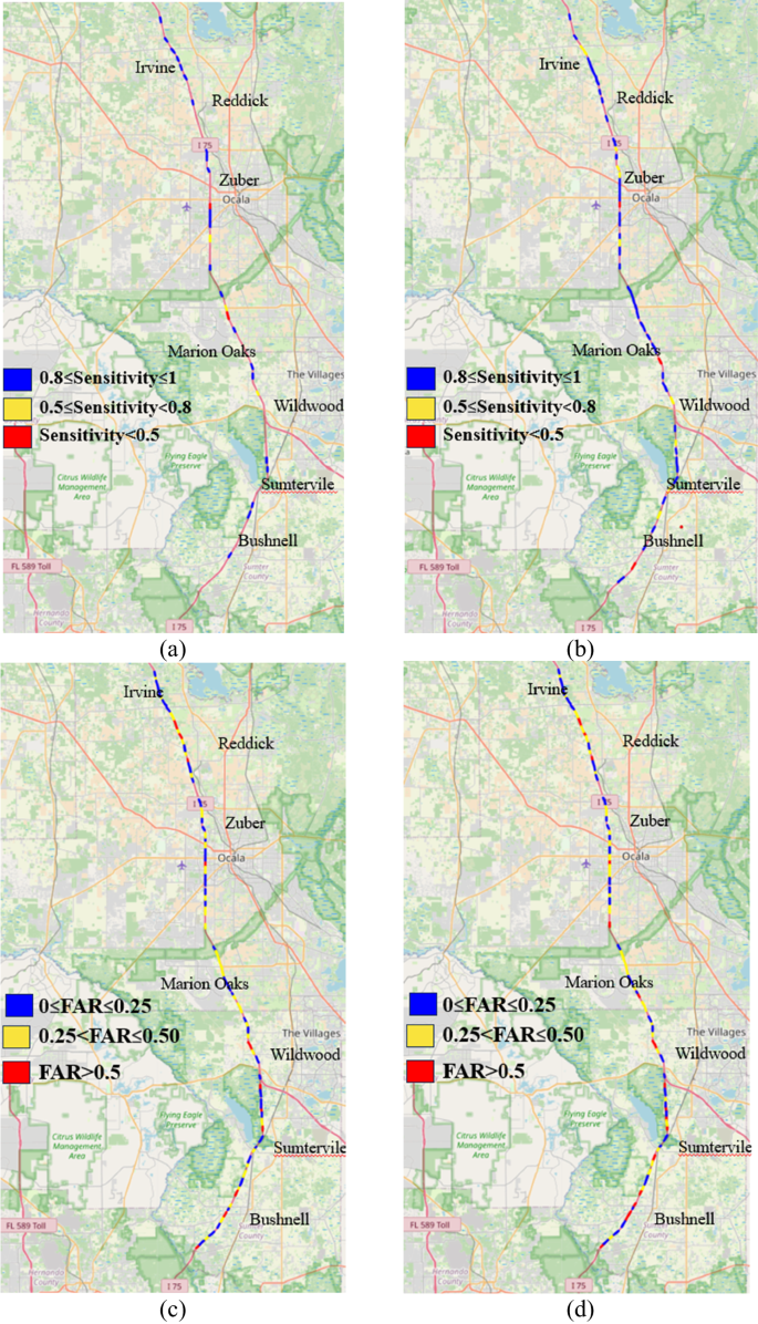
Blue indicates best optimization, i.e., highest sensitivity (tends to 1) or lowest FAR (tends to 0), while red indicates worse optimization, i.e., lower sensitivity or higher FAR. a Sensitivity for Minor Injury crashes, b Sensitivity for PDO crashes, c FAR for Minor Injury crashes, d FAR for PDO crashes.

Full size image

Installing detectors in close gaps on such segments might provide more accurate traffic information, and hence would increase the prediction performance. Finally, we link the traffic data property to this data feature pattern since higher fluctuations in traffic parameters make it hard for good prediction. Accordingly, it is suggested that improvement in the sensitivity and accuracy of the sensors in these regions may be helpful to more accurate prediction modeling.

Contributing factor analysis

We conducted an ablation study to investigate the sensitivity of different features to crash and severity prediction effectiveness. The results are presented in Table 5, where W/O indicates excluding (without) specific data features. When more important data features are excluded, more severe model degradations are expected. It is assumed that the traffic features will have a higher impact in predicting crashes and severity compared to weather data, and hence, this ablation study was conducted for traffic features only. Given the ablation study results in Table 5, it is shown that excluding traffic data has more effects on model degradation. Moreover, FAR was found to show higher variation after excluding different features compared to sensitivity and accuracy. The results from this ablation study in Table 5 show that the exclusion of volume data results in more severe model degradation. This implies that volume variable features play a more important role in crash and severity prediction. The rationale of such findings is justified by the literature as in low traffic volume conditions, drivers pay less attention to their own vehicle speed and there is a general tendency to speed. In such low volume-high speed conditions, crashes are more likely to be severe^40,56.

Our study developed reliable crash and severity prediction models by considering heterogeneity modeling, model generalization, and severity scale calibration. This work not only outperforms existing approaches and tackles unresolved challenges, but it also provides valuable insights into traffic system management, especially highway safety improvement. Some preventive measures, e.g., variable speed limit and queue warning, can be implemented in real-time to reduce the likelihood of crashes or their severities. The findings imply that traffic volume has the potential in detecting early warning signals for crash incidents across the studied segments. Given that our study operates on a lead time of 5–10 min, there is enough time and substantial potential for a significant reduction in crashes, particularly if the active traffic management strategies are adopted by the traffic management center (TMC). Dynamic speed limit, variable message sign, adaptive ramp metering, part-time shoulder use, and dynamic merge control are some of the suggested ATM strategies to avoid crashes or minimize the severity levels. For example, once the TMC receives notification of an increase in crash likelihood on a particular roadway segment, instantly, TMC can adopt ATM strategies for the upstream segments of the potential crash location, i.e., TMC could reduce the speed limit for the upstream segments from that crash location. This ATM strategy could help traffic avoid that certain crash-prone condition (time and location where the crash was supposed to occur) and hence, will avoid that crash or reduce its severity. However, the current study encourages further research to assess the effectiveness of different ATM strategies in avoiding different crashes and severities in real-time. Moreover, our model outperformed other existing models on false alarm rate, and this advantage can contribute significantly to minimizing the required installation efforts, i.e., lower false alarms can help provide more effective warnings and save warning triggering costs. Meanwhile, our models show more reliable results in predicting severe crashes. Thus, we are able to also predict segments projected to experience the most severe crashes and would prioritize additional preventive measures, e.g., variable speed limits coupled with queue warning or ramp metering. Finally, our system could suggest to policymakers to invest in ATM systems or develop new policies to avoid crashes or minimize their severity in real-time based on the real-time crash and severity prediction.

Since our algorithm is generic, it would be very feasible from a real-world deployment perspective to integrate this model with any traffic safety planning system. Figure 5 explains the framework of real-world deployment of our proposed real-time crash prediction along with their severity levels. First, real-time traffic and weather data will be streamed directly from the server controlled by the TMC. Then, our proposed modeling technique will be applied to predict the crash likelihood and crash severity. Finally, if there is a likelihood of a crash occurrence, TMC will be notified instantly with potential crash likelihood along with their crash severity levels. The intention is that TMC would take instant actions to prevent or avoid the crashes in minimal time based on the predicted crash severity levels. These actions include variable message signs, variable speed limit, ramp meter, even in case of fatal or severe crashes and direct notification to the potential crash-prone vehicle. Thus, our proposed system should be able to avoid or prevent crashes.

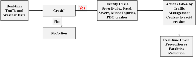
Real-world deployment of real-time crash and severity prediction framework with CCL.

Full size image

However, several potential challenges remain. The first involves optimizing the process of model update. As observation data increases, more features can be incorporated for predictive accuracy improvement. It is necessary to explore how to efficiently perform model retraining to leverage the increasing features. The second challenge is model robustness evaluation. In datasets with significant noise, such as failure of loop detectors, severe model degradation can result from this interference. Thus, exploring robust severity modeling becomes crucial under such circumstances. Also, communication latency during real-time implementation must be examined and addressed carefully. For example, TWC may fail to receive real-time inference results. Tackling this challenge is necessary to secure reliable severity prediction.

In this study, we also investigated the possible benefits of the computation efficiency of the developed model. The experimental findings indicate that the distilled model indeed improved prediction speed. This improvement is attributed to the reduction in the model configuration. The structure is reduced from a 10-layer MLP in the original teacher model to a 3-layer MLP in the distilled model. While the speed enhancement may not be substantial, it positively impacts the overall inference speed. Since this work focuses on the development of a generic algorithm, model and data, scaling-up has not been conducted. In the future, when larger-scale models are performed, the inference time reduction from knowledge distillation can be more significant, leading to more efficient prediction models for real-world applications.

This study is also in congruence with the United Nations (UN) sustainable development goals (SDGs) and is an attempt to help the stakeholders of SDGs to achieve its’ targets^70,71,72. Particularly, the current study proposes a novel and more sustainable solution to predict road traffic crashes along with their severity types, i.e., whether the crash is going to be a fatal, severe, minor or property damage crash only, even before the crash occurs. To materialize this concept into real-world implementation, this study applied innovative techniques, which is encouraged in SDGs^69,71,72. Furthermore, our proposed approach is designed with the objective of minimizing the carbon footprint, facilitating energy-efficient deployment for real-world applications⁷³, specifically in the context of real-time crash prevention and management, and reducing the impact of incident-related congestion^40,59,74. The sustainable deployment of our proposed methodology, focusing on computational energy efficiency in real-world scenarios, has substantial potential to actively prevent and mitigate crashes through the implementation of environmentally conscious traffic management strategies in real-time. This will reduce the number of deaths and minimize the socio-economic losses from road traffic crashes, and thus, will ensure a safe, reliable, resilient, and sustainable transportation system to achieve the UN sustainable development goals.

Overall, this study is the first in the literature to develop a real-time crash likelihood and crash severity prediction framework in a single system and present a deployment mechanism for real-world application. The study collected real-time traffic data from MVDS detectors installed on 67.6 miles section with 97 segments of I-75 freeway in Florida and real-time weather data from visual crossing. After proper data cleaning and preparation, the training dataset contained 67 million observations, and the test dataset contained 27 million observations with only 30 readily available real-time features. Then this study proposed a novel spatial ensemble distillation modeling technique to alleviate non-IID problems arising from heterogenous crash distribution and disproportionate samples for different crash severity levels, reduce the computational cost, make it flexible for missing data, enhance model accuracy, improve sensitivity, and most significantly reduce FAR. The modeling was performed in three different layers. First, a real-time crash likelihood model was developed to distinguish crash events from non-crash events in real-world situations. Second, the developed real-time crash likelihood model was tested with different crash types to ensure its viability in predicting different crash types. Finally, a real-time crash severity model was developed to predict the severity of crashes into four levels. Modeling results show that our proposed modeling technique efficiently predicted crash likelihood along with crash severity levels, reduced the model size, improved the sensitivity and accuracy, and significantly minimized the FAR. Particularly our developed models can predict fatal crashes with 91.70% sensitivity and 17.40% FAR, severe crashes with 83.30% sensitivity and 21.90% FAR, minor crashes with 85.6% sensitivity and 26.3% FAR, and PDO crashes with 87.70% sensitivity with 28.70% FAR, for all crash types. Similarly, it showed excellent performance for specific crash types, i.e., rear-end, sideswipe/angle. We also identified prediction challenges across locations, investigated the sensitivity of different features to crash and severity prediction effectiveness, and provided useful information for the modelers. Finally, we discussed the traffic safety improvement aspect, explained the real-world implementation mechanism, and highlighted the computational efficiency of our proposed methodology to avoid crashes or minimize crash severity.

The current study selected the southbound mainline of Interstate-75 (I-75) from District 5 of Florida, USA, as a study zone. It connects the south-west of Florida to the northern states of the USA and is considered to be a major route for connecting major metropolitan cities of Florida. The length of the considered roadway is 67.6 miles, and we collected data from 97 segments of this roadway.

Data processing

The current study used three data sources, i.e., crash data, traffic data, and weather data, to conduct this study. Signal Four Analytics (S4A) and State Safety Office Geographic Information System (SSOGIS) were used to collect 3 years (January 1, 2019–June 30, 2022) crash data. Both S4A and SSOGIS were used to collect the most comprehensive information of any crash and verify that information by comparing each other⁵⁶. Microwave vehicle detection system (MVDS) detectors installed on the I-75 update traffic information, i.e., speed, volume, and lane occupancy, every 30 s, and we obtained access to the traffic database through the Florida Department of Transportation (FDOT). These detectors are very closely spaced, and on average, their spacing is 0.51 miles. Weather data was obtained from a private stakeholder, visual crossing, which provides comprehensive real-time weather data.

Crash, traffic and weather data were matched and integrated together based on the useful features provided by these sources. Crash data obtained from S4A and SSOGIS contains comprehensive crash information, including crash date, time, year, latitude, longitude, crash type, and crash severity. Crash type variables information regarding different crash types, i.e., rear-end, sideswipe/angle, and crash type variable, provides four levels of crash severity, i.e., fatal crashes (K), severe crashes (A), minor injury crashes (B and C), and PDO/non-injury crashes (O). 30 s interval traffic data obtained from MVDS detectors were aggregated over 5 min for each road segment to generate some useful traffic flow attributes, i.e., average, standard deviation (SD), and coefficient of variation (CoV) of speed, volume, and occupancy. Here the road segment is defined by the intermittent roadway portion in between two MVDS detectors. For developing real-time models, the current study used traffic information from the target segment (where crashes occur), immediate upstream segment, and immediate downstream segment. Then the traffic information was integrated with the crash based on the crash location (latitude, longitude) and crash time (crash date, time, year). To avoid the effects of turbulence in traffic state⁷⁵ after a crash occurrence⁷⁴, information 1 h after any crash was discarded⁷⁶. Finally, the weather data was incorporated with crash and traffic data, and three weather variables, i.e., precipitation, visibility, and cloud coverage, were used in this study^77,78. Thus, we have complete real-time traffic and weather information for each crash in each segment of the freeway considered. The complete dataset contained 30 readily available real-time traffic and weather features, and they are as follows: 9 traffic variables per segment, i.e., 5-min average, SD, and CoV of speed, volume, and occupancy, and 3 weather variables are used, which yields 3 segments × 9 traffic variables + 3 weather variables equaling 30 features.

To predict the crashes in real-time and separate the crash events from non-crash events, the Crash prediction index (CPI) was used as the target variable. CPI was coded as a binary crash indicator to resemble crashes as 1 and non-crashes as 0. To explain the labeling of crashes and non-crashes more legibly, Fig. 6 is illustrated. If a crash occurred at 3:30 p.m., then the prior 5–10 min (3:20 p.m. to 3:25 p.m.) data was labeled as 1. Since these are 5 min aggregated traffic data, 5–10 min aggregated traffic information were processed from 5–10 min (3.25 p.m.), 6–11 min (3.24 p.m.), 7–12 min (3.23 p.m.), 8–13 min (3.22 p.m.), 9–11 min (3.21 p.m.), and 10–15 min (3.20 p.m.) traffic information. Hence, for a single crash, six CPI were labeled as 1 (crash) and the rest of the data were labeled as 0 (non-crash).

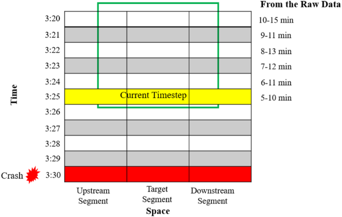
Crash and non-crash data labeling during data processing.

Full size image

The crash data used in this study four crash severity levels, i.e., fatal crashes denoted by K, severe crashes denoted by A, minor injury crashes denoted by BC, and property damage only (PDO) crashes denoted by O. This severity information was given by crash severity index (CSI) variable, and for modeling purpose, PDO was coded as 0, BC was coded as 1, A was coded as 2, and K was coded as 3. For clarification, CPI was used as the target variable in the first layer of real-time crash likelihood prediction. Then the crash severity of predicted crashes was further predicted in real-time crash severity prediction model, and CSI was used as the target variable in the later case. In both cases, the same 30 real-time traffic and weather features were used.

Finally, before using data into models, a further check was made to remove the missing data rows for these 30 real-time features and target variables. were removed. Also, the outliers were removed as per the suggestions of previous real-time literature, and three conditions were used to detect and remove the outliers. First, if occupancy was >100, and speed was equal to 0; second, if speed was greater than 100 and flow was >25/30 s; and final condition to detect outlier was if the flow was equal to 0 and speed was >0⁷.

We prepared training/testing time series for crash and severity prediction in machine learning. Adhering to the convention of time-series analysis and forecasting, data were partitioned into observation and forecasting time series. The observation period indicates the time windows during which data were collected and observed for analysis and modeling. The forecasting period refers to the time windows for which estimates were made with the model trained with data from the observation period. Following the machine learning time series convention, data sampled over the observation period were used for model training, and the crash/non-crash data in the forecasting period were employed for model testing. Therefore, forecasting model evaluation is reported based on the forecasting period. We employed supervised learning to develop a forecasting model where the input features were 30 variables, and the output label was CPI for crash likelihood prediction and CSI for crash severity prediction. Earlier studies employed different approaches for the train-test split. Some studies split based on the time, i.e., a specific time for training and another specific time for test data³². Some studies split based on the road, i.e., one road for training and another road for testing³⁹. Some used some popular percentages or ratios to data in the train-test dataset, i.e., 70–30%, 75–25%⁷⁹, 80–20%⁸⁰, and 10-fold cross-validation. The current study split the observation/training data and prediction/test data based on the specific time period. The observation period starts from January 1, 2019, to June 30, 2021, while the prediction period starts from July 1, 2021, to June 30, 2022^38,81. After this separation, the training dataset in the observation period contained 2080 crash events (CPI = 1) and 66,997,275 non-crash events (CPI = 0), where 40.53% were rear-end crashes and 25.91% were sideswipe and angle crashes. The test dataset in the forecast period contained 1035 crash events (CPI = 1) and 27,099,425 non-crash events (CPI = 0), where 47.93% were rear-end crashes and 20.87% were sideswipe and angle crashes. The exact same training dataset was used to develop models for all crashes, rear-end crashes, and sideswipe/angle crashes. However, to test the viability of the developed models in predicting rear-end crashes and sideswipe/angle crashes, only rear-end crashes + non-crashes and sideswipe/angle crashes + non-crashes data were used, respectively.

Spatial ensemble modeling for confidence calibration learning

First, we developed a zonal expert model for each individual segment. Then, we ensembled the zonal expert-trained model. Finally, we weighted the segment models for prediction. Multilayer perceptron (MLP) was used to develop individual segment-level models⁸² for its flexible input data structure. MLP allows input data to be vectorized and fed into training without specific formatting. This is very important in the real-time deployment of any such framework since, in many cases, detectors might have issues to provide continuous data, and we will have missing timestamps. Other proposed techniques for real-time crash likelihood predictions, like convolutional neural networks (CNN) or long short-term memory (LSTM) cannot deal with such circumstances. Another advantage of using MLP is that it even allows to addition of more layers or increased width without any alteration to input data. We used 10 fully connected layers and mean squared error (MSE) loss to yield both CPI and CSI. The MLP model architecture used in this study is shown in Fig. 7. Crucially, this lightweight model allows for faster training compared to larger models, especially on large-scale datasets. This efficiency conserves significant training resources and reduces carbon footprints, presenting a novel, efficient, and previously unexplored aspect in transportation modeling.

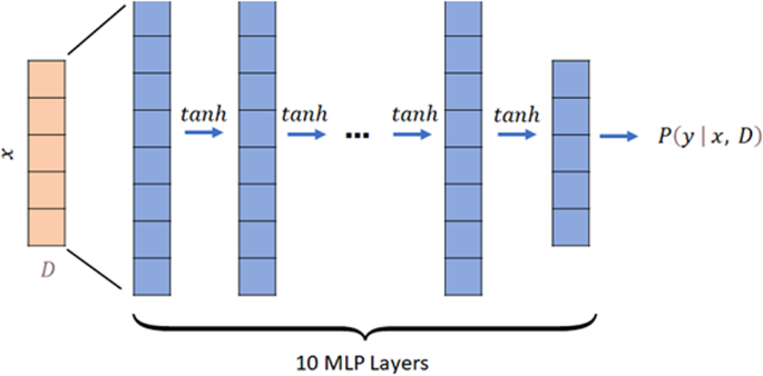
D represents datapoint and x is selected features. Each data feature vector is fed into a 10-layer MLP with tanh active function. The final output is a scalar P which indicates the probability of crash or level of severity.

Full size image

In the process of data preprocessing, the emergence of data discontinuity poses a challenge for temporally continuous modeling. The conventional modeling paradigm often addresses this issue through data imputation. However, it was recognized that such an approach carries the potential of introducing data bias during training, which is a notable concern in the context of machine learning applications and real-world implementation. As a result, we opted for a cross-sectional modeling approach, and specifically, a neural network in the form of a multilayer perceptron (MLP) was chosen for implementation. Specifically, the MLP in our implementation takes as input a set of 30 features, comprising 27 traffic-related features and 3 weather-related features. The output of the MLP is a binary crash/non-crash label, assessed with a 5-min lag. If a data point at a particular time step lacks information for all 30 features during training, it is excluded from the training set; during the evaluation phase, missing features undergo conventional linear interpolation to align with the model’s input requirements. Importantly, our crash labeling window extends to 10 min before the observed crash event. This indicates that the MLP model demonstrates proficiency in predicting crashes before 10 min, showcasing its robust capability for real-time crash prediction.

As a well-recognized measure of real-time prediction models, we used accuracy, sensitivity and FAR to measure the performance of our proposed models. Equations (7)–(9) define these three measures, where true positive (TP) denotes the number of correctly predicted crashes, true negative (TN) refers to the number of mispredicted crashes, false positive (FP) refers to the number of correctly predicted non-crashes and false negative (FN) refers to the number of mispredicted non-crashes⁴⁰.