Cascading socio-economic and financial impacts of the Russia-Ukraine war differ across sectors and regions

Severe disruptions in global trade and supply chains, particularly involving essential commodities like energy and food, can trigger far-reaching consequences across economies and financial systems worldwide. These disruptions, which may stem from various causes including geopolitical conflicts, can lead to cascading shocks through economic and financial systems, potentially amplifying impacts on key sectors and spreading losses to remote regions not directly affected by the initial trigger. The recent Russia–Ukraine war is an example that triggered severe disruptions in energy and food markets. The effects of the war on global energy and food trade, and how they propagate into the economy, finance, and private households can be conceptualized as a system of cascading shocks (illustrated in Fig. 1). A comprehensive assessment of such shock cascades and their potential amplification is relevant to design resilience policies and avoid systemic risks^1,2,3,4,5. However, a standardized approach to quantify cascading impacts from trade and supply disruptions and the relevance of their potential to amplify losses at the sectoral and geographical level has been missing up to now.

Disruptions in energy and food supply and trade, affect energy and food price inflation in the real economy. On the financial side, the war also changes market expectations, leading to higher prices for energy and food commodities in future markets, which then amplify energy and food price inflation. Both the real and financial shocks affect energy and food security for households and firms and also propagate into companies’ stock prices and investors’ portfolios. The graphical representation of cascading impacts builds on the conceptual framework of Carter et al.², where red triangles indicate the initial impacts, red arrows the impact propagation channels, blue squares the affected system components, green triangles recipient systems of the impacts, and green arrows policy responses.

Full size image

We fill this gap by providing a methodology that enables us to assess the cascading impacts of trade and supply disruptions across economic, financial and food systems, considering the amplification effects in financial markets. Here, amplification denotes the increase in magnitude of economic shocks, driven by financial market responses to the original shock. We test our methodology using the Russia–Ukraine war as a case study, given that both belligerents are major actors in the global food and energy trade. We analyze the impacts of several commerce-related measures on Russia and the disruptions emerging far from the war and consider the potential overreaction stemming from financial markets. In our approach, we first assess the macroeconomic impacts of a stylized representation of the war with the ICES computable general equilibrium (CGE) model^6,7,8. Applying a CGE model enables us to fully integrate productive sectors and countries through international trade and to capture the complex economic dynamics of moving from one economic equilibrium to another as a consequence of a shock, such as a war. Second, we capture abnormal financial reactions of commodity markets with an event study analysis, carrying out an empirical analysis of the impact of the war on commodity prices^9,10,11. These abnormal reactions originate from violations of the efficient market hypothesis, according to which asset prices reflect all available information and thus adjust to events without overreaction¹². Third, we quantify cascading effects on global companies and investors. Fourth, we apply a food affordability analysis to quantify the impacts on different income groups of private households. The analyses on companies, investors, and private households are conducted for two cases: one based solely on macroeconomic impacts, and another combining these with abnormal financial market reactions, quantifying the amplification effect of financial markets.

Interestingly enough, available evidence enables us to verify how much our methodology captures observed facts. Recent research showed that globally, as a result of the war, GDP was estimated to shrink between 0.7% and 1.5%^13,14,15,16 and global inflation to rise between 1.0% and 2.5%^15,17 within one year since the outbreak of the war. Estimates agree on high losses for Russian welfare in the range of 4.0−14%^{14,17,18,19,20,21}, and for the European Union (EU) in the range of 0.2−5.0%, particularly in Eastern Countries, due to a higher import dependency on Russian energy products^22,23,24. The estimated welfare or gross domestic product (GDP) reductions mostly result from energy supply reductions and increasing energy prices^17,25,26. Higher prices, in turn, decrease the production of energy-intensive goods and services. Countries that are net energy and agricultural importers, such as Turkey, Thailand, and South Africa will hence be negatively affected. Moreover, the ban on Russian fertilizers negatively impacts countries whose economies are tightly linked to agricultural production and export, such as Brazil, the world’s largest soybean producer. This, in turn, triggers further cascading effects, e.g., on China, which imports Brazilian soybean for animal feeding, leading to a rise in world meat price¹³. At the same time, marginal positive impacts are expected on the US and several Western economies^18,20,27 benefiting from replacing Russian and Ukrainian suppliers, such as in the cereal and oil seed markets²⁸. Other benefits are expected for countries that are not involved in the war, such as India^21,29, and specific groups, like crude oil producers¹³. The literature shows that financial markets reacted in very different ways to the invasion of Ukraine across regions and economic sectors. European stock markets suffered the most, followed by Asian stock markets, while the reaction in the US has been milder^30,31,32. Overall, at the sector level, energy markets have outperformed other equities, especially in the US³³. Renewable energy markets reacted positively^34,35, though green stocks did not show positive returns³⁶. Different behavior at the sector level can be explained by heterogeneous changes in expectations with respect to the energy transition³⁷. Other markets have also shown highly heterogeneous reactions following the invasion (e.g. currencies³⁸, cryptocurrencies³⁹, or metal markets³⁵). Nevertheless, the consequences of the war on commodity markets have received little attention so far in the literature, with the notable exception of renewable energy, conventional energy, and metals³⁵. Besides their effects on the real and financial economy, conflicts are currently among the most important drivers of food insecurity globally^40,41,42. The ongoing Russia–Ukraine war has worsened existing food insecurity, compounding with the effects of the COVID-19 pandemic, climate change, and rising economic inequality^{42,43,44,45,46}. The war not only led to supply disruptions but also put pressure on grain market prices, thereby impacting economies with limited fiscal resilience to price shocks. Projected food insecurity risks vary strongly: the United Nations’ Food and Agriculture Organization (FAO) estimates that an additional 8-13 million people are at risk^47,48, Arndt et al. expect 22 million people⁴⁹, while the World Food Program (WFP) estimates an additional 47 million at risk of undernourishment⁵⁰. Various methods have been applied to assess the impacts of shocks on food security, ranging from descriptive^{44,51,52,53,54}, econometric⁴³, CGE models with explicit consumer classes⁴⁹, and network-based approaches^55,56. There is extensive agreement that import-dependent low- and middle-income countries^{44,51,52,53,55} are most vulnerable.

Examples are highly import-dependent regions in the Middle East and North Africa^56,57, but also the Sahel region^44,51,53.

Here, we complement the insights of such analyses by providing a comprehensive and cross-sectoral assessment of the cascading impacts of the global trade disruption by the geopolitical crisis. We have chosen this case study for its complex economic, financial, and social repercussions, and for the possibility to compare our findings with the evidence. Our methodology extends beyond this specific case. Our study goal is to provide a methodology that can account for any shock, including climatic events, where global trade of key commodities is disrupted. It allows us to study the cascading impacts across sectors and geographies on macroeconomic variables, such as adjustments in trade patterns, production, and GDP, as well as on financial variables and potential amplification effects, and impacts on companies, portfolios, and on private households. In the case of the Russia–Ukraine war, such cascading impacts are primarily triggered by a shock in the energy and food trade. We define a war scenario that mimics the key features and likely consequences of the war over the year 2022 (see the “Methods” section). It incorporates the immediate destructive effects of the Russian invasion on Ukraine’s productive system, the commerce-related measures imposed by the Western block countries towards Russian products, and trade disruption (for a detailed description, please see Table 1). It is important to note that our scenario was created before actual commerce-related measures were implemented and does not consider the effects of sanction evasion, the increase in war-industry production, or the outcomes of international negotiations. Further, our methodology integrates empirical data for commodity markets around the invasion date. Our results enable us to tackle cascading impacts into three dimensions of the crisis: macroeconomics, valuation of companies and investors, and food affordability. We capture the macroeconomic consequences of the Russia–Ukraine crisis, such as changes in trade patterns, domestic production, GDP, and prices (see section “Macroeconomic impacts of the conflict: GDP, trade, and commodity prices”). Next, we assess the ramifications on company valuations and investors’ portfolios (see section “Financial impacts: commodity and equity shocks”). Finally, we quantify the effect on food affordability for private households (see section “Impacts on food affordability across income groups”). To make the financial amplification effect explicit, we analyze the impact on companies, portfolios, and private households for two cases: the base case and the financial amplification case. The base case describes impacts purely stemming from the macroeconomic analysis. The financial amplification case extends the analysis and combines sectoral performance values from the base case with empirical futures market data from which we derive the abnormal reaction of selected commodity prices due to the invasion. To further illustrate the differences in how the two cases manifest through selected commodity price changes, we provide an explicit comparison in the section “Analysis of price amplification effects on selected commodities”. Given the extensive results from our multidisciplinary approach, further details are available in the Supplementary Information.

Macroeconomic impacts of the conflict: GDP, trade, and commodity prices

Here, we present the main macroeconomic impacts (see also Fig. 2). For a detailed sensitivity analysis of the role of the key model’s parameters (i.e. Armington elasticities and supply elasticities for fossil fuels) on macroeconomic results, refer to Supplementary Information Section 2.1.

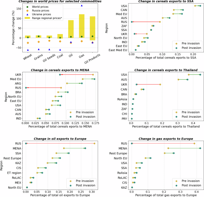
Top left panel: bar chart showing world prices (green dots) and ranges of regional prices (yellow bars) for selected agriculture and energy commodities w.r.t. reference year. Orange and blue markers identify price changes for Russia and Ukraine respectively. Note that Ukraine gas price spikes affect <1.0% of the World gas supply. Top right and mid left and right panels: lollipop charts showing changes in cereals exports (in value terms w.r.t. reference year) towards Sub-Saharan Africa (top right), MENA region (mid left) and Thailand (mid right) of top-10 exporters by region before and after invasion. Bottom left and right panels: lollipop charts showing the changes in oil (left) and gas (right) exports (in value terms w.r.t. reference year) towards the EU of top-10 exporters before and after the invasion. List of acronyms used in the up, mid, and bottom panels: ARG Argentina, AUS Australia, BRA Brazil, CAN Canada, CHN China, CIS Commonwealth of Independent States (except Kazakhstan), IND India, KAZ Kazakhstan, PRY Paraguay, MENA Middle East and North Africa, MEX Mexico, RoAsia Rest of Asia, RoLAC Rest of Latin America and Caribbean, RUS Russia, SSA Sub-Saharan Africa, ET region Euphrates-Tigris region, UKR Ukraine, ZAF South Africa.

Full size image

Real GDP losses induced by the war mainly concentrated in Russia (real GDP loss of 14.0%) and Ukraine (real GDP loss of 53.0%) over one year (Supplementary Fig. 1, bottom panel). The EU (see Supplementary Table IX) experiences an average real GDP reduction of 0.8% (Supplementary Fig. 1, top panel). Higher losses (ranging between 1.4% and 1.8% of real GDP) occur in the Eastern EU countries, such as the Baltic states, Poland, and Bulgaria, as a consequence of their higher dependency on Russian fossil fuel imports, especially gas. Outside the EU only Japan faces a modest −0.2% reduction in GDP for 2022, while GDP increments are suggested for CIS countries and Kazakhstan (nearly 0.3% in both cases). For other countries, GDP effects are almost null, in the range of +0.1%/ −0.1% (Supplementary Information subsection 2.1). As Russia reduces gas exports towards the EU to zero, the supply gap is closed by imports from other countries: the MENA countries (compensating for 52.0% of Russian reduction), the European Free Trade Area (EFTA) (for 16.0%), the US and the Northern EU countries (for 9.0% and 8.0%, respectively) (Fig. 2, bottom right panel). Similarly, Russian oil exports towards the EU fall to zero and the gap is closed by imports from the MENA region (compensating for 42.0% of Russian reduction), sub-Saharan Africa (for 27.0%), EFTA countries (for 17.0%), and the Commonwealth of Independent States (CIS) (for 14.0%) (Fig. 2, bottom left panel). Conflict and commerce-related measures put inflationary pressure on global energy prices, which increase between 6.2% and 8.5% (see Supplementary Information subsection 2.1 for a detailed analysis of World prices). The EU is particularly affected by spikes in energy prices. On average, oil prices rise by 32.0% (with peaks of 13.0% and 91.0% in the Mediterranean and in the South-Eastern EU, respectively), while gas prices increase by 26.0% (between 11.4% and 121.0% in the South-Eastern and Eastern EU, respectively). Coal prices are much less affected with only a noticeable 8.5% increase in the Northern EU (Fig. 2, top left panel). Higher energy commodities’ costs affect electricity prices (maximum price boost of 10.5% in the Eastern EU), and to a lesser extent, energy-intensive industries where price spikes are lower than 2.0% with the exceptions of the “iron and steel” sector in the Eastern EU (+6.1%) (Supplementary Fig. 3). Agricultural commodity markets are also particularly sensitive to the war’s effects because both Russia and Ukraine are major agronomic players. Cereal world prices rise by nearly 9.0%, that of wheat by 3.0%, and that of other agricultural commodities by 2.0% on average (Supplementary Fig. 2). It is worth stressing that, in our scenario, the agricultural sector is affected by the ban on Russian exports of fertilizers as well. Inflationary pressures in the food sector are most harmful to poorer households in low-income countries, such as in the Middle East and Northern Africa (MENA) region and sub-Saharan Africa (SSA). However, poorer households in higher-income countries can also be affected. These two regions largely depend on imports for several agricultural products, such as cereals. Russia ranked 5th and 4th as exporter of cereals for SSA and MENA, respectively, while Ukraine was the 8th and the 1st exporter of cereals for both regions according to ICES projections for 2020. After the Russian attack, cereal supply from Russia and Ukraine contracts and new trading partners start supplying. Indeed, the US, Canada, and the Mediterranean EU member states (e.g. Italy, France, and Spain) close the gap through their exports to SSA. The US and Canada provide nearly 72.0% of the gap. Similarly, in the MENA region imports from belligerents are replaced mainly by imports from South American countries, the US, and the Mediterranean EU countries (Fig. 2, mid left panel for MENA and top right for SSA). Also Asian countries, such as Thailand, have been dependent on Ukrainian cereals. Before the war, Ukraine was the 3rd cereal supplier (mainly for wheat) providing nearly 20.0% of total Thai cereal imports. The war started, Ukraine was supplying only 3.0%. The gap in cereal imports was closed by three countries: the US, Australia, and Canada. Before the war, they supplied 74.0% of Thai cereal imports; since the war started, their joint supply reached 90.0% (Fig. 2, mid-right panel). International trade mechanisms and the existence of several cereal trading partners stabilized agricultural prices in SSA and in the MENA region where they increased a rather moderate +2.8% and +4.0%, respectively. Given a lower possibility to diversify suppliers, Thai cereal prices increased by nearly 6.0% (Supplementary Fig. 3).

Financial Impacts: commodity and equity shocks

The extensive results of the event study are presented in Supplementary Table II. They show strong and heterogeneous overreactions in commodity markets. Here, we report the main results. Notably, gas contracts using the Title Transfer Facility (TTF) in the Netherlands and the National Balancing Point (NBP) in the UK as pricing points show very strong overreaction to the invasion (+67.47% and +72.78%, respectively). On the contrary, contracts priced on US gas markets are unaffected, with the Henry Hub and other regional pricing points (e.g. the Algonquin Citygate in New England and the Chicago Citygate) showing no overreaction. Regarding agricultural commodities, wheat shows the strongest overreaction, especially the futures priced in Chicago (+44.66%) and Paris (+33.35%). Smaller reactions are detected for futures priced in South Africa (+17.61%) and China (+13.12%). The overreaction of corn markets is smaller (+14.53% for futures trading on Argentinian corn, +9.05% for futures trading on Chicago). Other agricultural commodities show no significant overreaction (soybeans, rapeseed, cocoa, sugar), or a negative overreaction (Chicago live (−5.66%) and feeder (−8.02%) cattle, US coffee future (−17.99%)).

The event study enables us to quantify the overreaction in commodity markets (see the “Methods” section) and thus, leveraging a dividend discount model, the company- and portfolio-level results, including the financial amplification (labeled finance amplification case). In the following, we compare these results to the ones without financial amplification (labeled as base case) in Figs. 3 and 4.

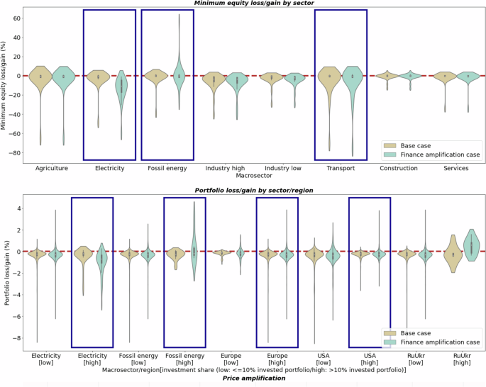
Top panel: violin plot showing the (estimated) distribution of minimum equity losses/gains for companies in given groups of sectors. The distributions are estimated using a kernel density. The white dot represents the median of the data, the black box the interquartile range, and the lines the 1.5× interquartile range. Not all violins show all marks. Estimated maxima and minima may be different from model maxima and minima. The kernel density estimation shows the distribution shape of the data: a wider section represents a higher probability that members of the population take a given value, and a skinnier section represents a lower probability. Bottom panel: violin plot showing the portfolio losses/gains for investors with low (i.e., less than or exactly 10%) and high (i.e., more than 10%) shares of investments in a given sector/region. The violin plot is estimated using a kernel density. In the top and bottom panels, blue boxes are drawn to highlight the largest impacts. For a detailed discussion, please refer to the section “Financial impacts: commodity and equity shocks”.

Full size image

In the top panel of Fig. 3, electricity and transportation companies suffer stronger equity losses due to the increased fossil fuel prices (up to 59.9% and 75.22% equity losses in the base and the amplification case, respectively). On the contrary, fossil energy companies largely benefit (with equity gains up to 57.35% in the amplification case). Nonetheless, some fossil energy companies suffer equity losses (up to −28% in the amplification case). These effects can be observed at the portfolio level as well (bottom panel) where portfolios with high exposure to fossil energy (electricity) strongly gain (lose) in the finance amplification case (with portfolio gains of up to 3.70% and losses up to 4.89%, respectively). Other sectors undergo limited shocks because they are less dependent on commodities impacted by the war. Finally, we find that investors’ losses are heterogeneous across regions and sectors in both the base and finance amplification case (see Fig. 4 for the latter case). Investors with significant (>10%) portfolio exposure to Europe suffer up to 6.08% losses, while investors with large exposure to the US suffer only up to 3.10% losses.

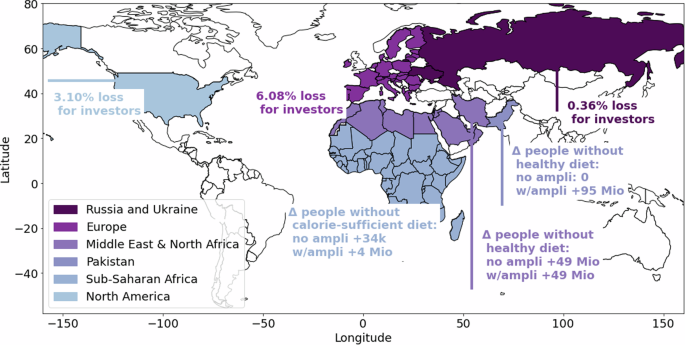
For financial results, the minimum loss for investors with more than 10% exposure to the highlighted region/country is shown. For food affordability, the amplification effect is depicted (“w/ampli” vs. “no ampli”) by the number of people that cannot afford a calorie-sufficient or healthy diet anymore (see subsection “Impacts on food affordability across income groups”). In sub-Saharan Africa, due to the amplification, the number of people who cannot afford a calorie-sufficient diet anymore rises from 34,000 to 4 million, and a healthy diet becomes unaffordable for an additional 95 million people in the rest of Asia. In the Middle East and North Africa region the number of people unable to afford a healthy diet remains constant at 49 million, as the price increase of the base case already made a healthy diet unaffordable.

Full size image

Analysis of price amplification effects on selected commodities

Here we compare the commodity price increases in the base and finance amplification cases with the real price increase recorded over 2022. Figure 5 shows the price increases in the base case (dark blue dots) based on ICES compared to those induced by the abnormal returns in the finance amplification case (cyan dots) and price changes for 2022 in future/spot markets (purple stars)⁵⁸, for commodities that are most relevant during the crisis. The price changes for 2022 are computed as the percentage change in price between a given future/spot on the first trading day of 2023 with respect to the first trading day of 2022. Note that additional factors, not considered in our scenarios, influenced the real prices over the course of 2022. Nevertheless, considering the overreaction of commodity markets strengthens the explanatory power of our analysis. For most commodities, the financial amplification effect is larger than the price increase in the base case, peaking at 80% in the case of the UK for gas. However, some commodities, notably oil, did not overreact despite the projected price increases by ICES. This heterogeneity across commodities stems from a combination of the importance of Russia and Ukraine in the global market and dependence on them, and investors’ sentiments. Overall, when comparing price increases in the base and finance amplification cases with the real ones, three groups emerge. The first group includes commodities where the real price increase is below the base and financial amplification prices, despite a strong initial reaction. This is the case of gas futures in all markets where an overreaction occurred (Europe, UK, Asia). The real price effect mostly stems from the reduction in demand induced by cutback efforts, a milder European winter⁵⁹, heavy subsidies to support energy and, in particular, gas demand⁶⁰, and inflow of liquefied natural gas (LNG)⁶¹. While the high prices did not persist, it is important to notice that price spikes reached up to 244% over the course of the year. Interestingly, in gas markets where no immediate overreaction was observed (e.g. the US market), the price at the end of 2022 was higher than the base case projection. The second group includes commodities where the real price increase is between the base and financial amplification cases, e.g. for European and US wheat. The initial price overreaction in these examples was subsequently curtailed by international efforts, such as the Black Sea Initiatives or the EU Solidarity Lanes, and demand destruction. It is important to note that, before stabilizing, real prices increased even more than the initial overreaction (Supplementary Fig. 11)⁵⁸. Oil represents a peculiar case for which no immediate overreaction is observed, but real price increases were lower than the ones projected in our base case. The third group includes commodities where the real price at the end of 2022 was above both the macro and amplification levels, see, e.g. corn, oil products, or US gas. This result is driven by real macroeconomic factors such as a lower production over the course of 2022, e.g. in the case of corn⁶².

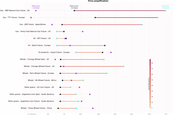
Comparison between price increases in the base case (“Base price increase”, dark blue dot), in the finance amplification case through abnormal returns from commodity future markets (“Financial increase”, cyan dot) and real future price increase over the year 2022 (“Real price increase”, purple star). Horizontal axis: percentage price increase. Vertical axis: selected commodities. Horizontal bars connecting the “base” to the “financial” price increase depict the amplification effect of financial markets. Source: authors’ elaboration on Refinitiv Eikon data.

Full size image

Impacts on food affordability across income groups

To illustrate the cascading effects on private households, we analyzed changes in food affordability for individuals. Specifically, we focused on the affordability of a calorie-sufficient diet, which is the basis for people suffering no hunger⁴¹, and a healthy diet, which ensures adequate levels of all essential nutrients⁴¹. Our analysis spanned across the income levels classified by the World Bank in ref. ⁶³ and the ICES regions (Supplementary Table IX). The results revealed an increased number of individuals unable to afford these diets due to price increases. Already at pre-war prices a calorie-sufficient diet was unaffordable for 140–360 million people and a healthy diet for 1.9–3.2 billion people, both in a lower and upper bound estimate (see also Supplementary Figs. 15, 16). Thus, price increases further strained those already struggling to meet basic food needs. Please note that the upper bound estimate additionally accounts for national variations in budget allocations, including essential non-food expenses. Analyzing the affordability of the diets for both the base and finance amplification case shows a pronounced rise in the number of individuals unable to afford a calorie-sufficient diet. The lower bound estimate reveals an increase from 0.16 million to 10.4 million people, from the base to the finance amplification case (65 times more people), while the upper bound estimate shows an increase from 4.89 million to 163 million people (33 times more people). The amplification affects especially people from lower-middle-income countries (classification from ref. ⁶⁴) (62−98%, lower and upper estimate) and from the perspective of individual income levels⁶³ especially extremely poor people (77−99%, lower and upper estimates) living from <2.15$ per day (2017 PPP). In the base case, mostly upper middle-income countries (26−99%, lower and upper estimate) and extremely poor people (73−99%, lower and upper estimate) were affected. In contrast, for healthy diets, the increase in the number of people affected is only seen in the near-poor income group (budget <6.85$ per day), as lower income groups were already unable to afford such diets at pre-war prices.

Switching to a regional analysis, notable differences between the base and finance amplification cases are revealed (see Fig. 4 and Supplementary Table IX for regional definitions). For a calorie-sufficient diet under the lower bound estimate, sub-Saharan Africa experiences an increase from 0.034 to 4 million additional individuals unable to afford this diet. Similarly, the Rest of Asia, particularly the Philippines, increases from zero to 5 million, and the Rest of Latin America and the Caribbean, especially the Dominican Republic and Honduras, from 0.088 to 1 million. In the upper bound estimate, Sub-Saharan Africa’s affected population rises from 4.7 to 19 million, India’s from 0 to 133 million, and both Eastern and Northern EU see an increase from 0 to 0.055 million. For a healthy diet under the lower bound estimate, the Rest of Asia, notably Pakistan (Fig. 4), sees an increase from 0 to 95 million individuals unable to afford it, while in Sub-Saharan Africa, the number rises modestly from 5.1 to 5.6 million. Conversely, in the Middle East and North Africa, as well as the Euphrates-Tigris region, the numbers remain unchanged at 49 and 7 million respectively, reflecting that prior price increases in the base case had already made a healthy diet inaccessible for some income groups.

Reality checks

To complement the price analysis in the section “Analysis of price amplification effects on selected commodities”, we further validate our results against real data as of one year after the invasion. Importantly, many economic circumstances have changed between the start of the invasion and the time of writing. These include, for example, the monetary tightening from the US Federal Reserve, which started in March 2022, or the policy efforts from the European Commission to counteract the negative effects of the invasion, to name but two. Hence, it is not possible to fully isolate the impacts of the invasion in the real world in the same way as we did in our modeling framework. Nevertheless, we aim to ensure a general consistency of our results with reality. Our reality checks are summarized in Supplementary Table III and further discussed in the Supplementary Information subsections 3.1–3.3.

From a macroeconomic viewpoint, trade-related variables, such as trade pattern shifts and price trends post-invasion, largely validate our model’s predictions while GDP changes, especially in belligerent countries, deviate from official statistics (for a detailed discussion see Supplementary Information subsection 3.1). The realignment of trade, particularly in agricultural commodities, mirrors World Trade Organization findings⁶⁵. Large reductions in Ukrainian exports and alterations in Russian trade dynamics, as corroborated by WTO⁶⁶, further reinforce these observations. Moreover, ICES outcomes on agricultural product prices align with data from the Food and Agriculture Organization⁶⁷ and the WTO⁶⁵.

Our financial results are also aligned with real data for 2022. Energy companies like Saudi Aramco or Royal Dutch Shell registered record profits⁵⁸. Similarly, exchange-traded funds (ETFs) linked to fossil fuels, such as the SPDR S&P Oil & Gas Exploration & Production ETF, experienced record highs. Conversely, sectors and companies dependent on fossil fuels experienced various degrees of losses^58,68. Performance has been mixed in the electricity sector, where some company’s equity value declined (e.g., in Europe), and others increased (e.g., in the US). Furthermore, companies with a high focus on renewable energy have shown a better performance than others highly reliant on fossil fuels⁵⁸.

The picture of heightened food insecurity, particularly in sub-Saharan Africa, the MENA and Euphrates and Tigris region is supported by insights of reports like the Global Report on Food Crises⁴⁵ and the Global Food Security Index⁴². Basing the analysis only on values as provided by the macroeconomic equilibrium model would have severely underestimated the additional people experiencing food insecurity. Additionally, the situation in the Philippines and Latin American countries like Honduras and the Dominican Republic⁴⁵ echoes the model’s findings on the adverse impacts of economic shocks on food security.

We developed and tested a methodology to assess cascading socio-economic and financial impacts induced by shocks on the global supply and trade of key commodities. By integrating macroeconomic and financial aspects we capture both direct and amplified effects on various sectors and regions that traditional methods might miss. We applied this methodology to study the consequences of the Russia–Ukraine war, focusing on the implications for food and energy markets. Our results highlight the heterogeneity of cascading impacts across sectors and regions outside Russia and Ukraine, with the emergence of distinct winners and losers.

A comparison with real data shows that our approach captures well the key impacts of the crisis in terms of direction and magnitude of impacts, such as the magnitude of the energy price increase in Europe, the gains of fossil fuel producers, and the worsening situation of food affordability (see reality checks in the section “Reality checks”). From the macroeconomic side, the large cascading effects that occur, especially in regions that are highly dependent on Ukrainian or Russian commodities’ exports, such as the EU and South East Asia (e.g. Thailand), are confirmed by official data. Negative shocks on the balance of payment emerge, as well as a deterioration of the countries’ GDP, sectoral outputs, and increases in prices. While trade patterns and prices react in line with official statistics, most GDP changes in one year of war generally point in the right direction with mild differences in magnitude. Only for the belligerents, Russia and Ukraine, the ICES CGE model suggests higher GDP losses, which we discuss below in limitations.

The financial analysis shows that companies and investors exposed to negatively affected regions (such as EU-based, non-fossil companies) suffer severe financial losses. In contrast, regions, companies, and investors that are less dependent on Russia and Ukraine emerge as winners. In particular, fossil fuel energy producers and their investors benefit from shifted fossil fuel production, oil and gas price increases, and abnormal returns on energy commodities. As our methodology looks at impacts on the agricultural sector, commodity prices, and food affordability of private households at the same time we can confirm official data that food prices harm consumers, especially the poorest households in import-dependent low-income countries (e.g., in Sub-Saharan Africa, Asia, and Latin America), but also relatively richer households (e.g., Middle East and North Africa, Euphrates-Tigris region, Sub-Saharan Africa). At the same time, rising food prices benefit the agricultural sector and agricultural producers, especially in Canada and the U.S. for wheat, and in several Latin American countries, such as Argentina and Brazil, for other cereals. Our integration of the amplification analysis for the financial and food sectors shows that unexpected disruptions can lead to overreactions in financial markets. It quantifies this amplification, demonstrating that neglecting financial market assessment in fundamental disruptions of global key commodity trade can lead to an underestimation of cascading impacts, especially due to market inefficiencies that can occur. Importantly, while our financial markets analysis is focused on the short-term effects of the crisis, the results are comparable with the 1-year observed effects in financial markets (both at the company- and portfolio levels). Crucially, our approach enables tracking and explicating the transmission mechanisms across different dimensions. This would not have been possible without the integration of the macroeconomic and financial analysis. For example, we not only identify the increase in food insecurity due to curtailed wheat exports from major grain exporters, but also track the full trade, financial, and price demand mechanisms leading to this outcome, disentangling the relative importance of each factor. Further, providing a differential analysis of food affordability along income groups of countries and private households can be highly relevant to prevent further cascading impacts. For instance, the relationship between income loss and violent mobilization is strongest among recently downgraded groups⁶⁹. This comprehensive understanding delivered by our methodology aids in devising better policy actions.

Policy implications and recommendations

Our analysis suggests that avoiding concentrated dependencies on individual trading partners and diversifying supply are key policy measures to reduce cascading risks. However, reducing dependencies does not mean curtailing trade. Our macroeconomic sensitivity analysis (see Supplementary Information subsection 2.1) supports that keeping trade open helps to mitigate supply shocks and increase resilience. Conversely, domestic production in some strategic sectors may also help cushion immediate shocks and provide time to redirect imports from other trading partners without suffering major losses (see also ref. ⁷⁰). For example, developing renewable energies could be a win–win strategy under this perspective.

Our study shows the importance of including cascading risk in the supervisory tool of financial authorities, such as central banks and financial regulators, in order to strengthen their financial risk assessment and risk management. In particular, our analysis shows that the consideration of cascading risks provides a more comprehensive picture of the losses for financial institutions, avoiding their potential underestimation. A better quantification of risk, in turn, is crucial for the design of prudential policies either at the level of individual financial institutions (microprudential policy), and of the financial system (macroprudential). This is shown by the results of our study, where companies and investors with higher diversification (in terms of supply chain and portfolio allocation) and lower dependence on Russia and Ukraine for their business are more resilient to the cascading effects of the crisis. Our food security analysis confirms the existential vulnerability of low-income populations to market uncertainties triggering price spikes in global markets^51,52,71,72, which highlights the need for financial authorities to consider the broader economic implications of financial market dynamics in their risk assessments. The analysis further stresses the key role of international collaborations and agreements⁷³ when it comes to reducing market uncertainties (e.g. the UN-brokered Black Sea Grain Initiative and the EU’s Solidarity Lanes Initiative⁷⁴). International cooperation should further provide targeted humanitarian aid through multilateral programs such as the UN’s World Food Program⁷⁵. Finally, windfall taxes, which are surtaxes imposed by governments on businesses’ excess profits, can be considered to counter negative redistributive effects on private households (as observed, for example, in response to the EU energy crisis^76,77).

Limitations

Acknowledging the limitations of our study, we note discrepancies in macroeconomic and financial outcomes due to modeling constraints, scenario setup, and sectoral aggregation. Modeling-related limitations include: (i) modeling re-exporting, (ii) economic agents behavior, (iii) the neoclassical assumptions, and (iv) the assumption on monetary and financial neutrality. Firstly, ICES, like any other CGE model, is not able to capture a re-exporting mechanism. In terms of our analysis, this translates into the impossibility to track Russian exports that bypass the bans through re-exporting via third countries, such as the case of India for crude oil⁷⁸. Then, CGE models often make simplifying assumptions about economic agents’ behavior, which may not fully capture the complexity of human decision-making. For instance, these models typically assume perfect information and rational decision-making, which may not always hold in the real world. Furthermore, ICES is based on a neoclassical paradigm and considers the transition from one equilibrium to another without considering abrupt changes in the very short run but smoothing trends over a longer period. This focus on longer periods prohibits understanding immediate reactions. Finally, ICES belongs to the class of “real ” CGE models that include only flows and transactions in the real side of the economy neglecting the role of monetary and financial phenomena. With respect to the scenario set up, we do not account for war-related sectors’ expansion, such as heavy industry or technological sectors or financial sanctions. Further, we omit some commerce-related measures, such as the prohibition on exports of EU dual goods, on EU imports of Russian gold and diamonds, or an arms embargo. Finally, the regional and sectoral aggregation affects the magnitude of the results but not the sign of changes in the main macroeconomic variables. Although most of our findings align with official records, the discrepancies in our modeling results for the belligerents’ GDP are primarily due to our scenario setup such as not including the expansion of war-related sectors and constraints on modeling re-exporting. For example, our model reports a more pronounced decline in Russian GDP compared to official figures. Drawbacks due to macroeconomic modeling constraints are partly countered by our analysis with the financial model which captures abrupt, immediate reactions and expectations. It approximates them utilizing excess returns, although it may miss nuances in intraday movements and broader investor impacts. The equity valuation is constrained by incomplete dividend data and a generalized view of companies by region and sector. Further, our approach primarily reflects European equity data, offering only a partial view of financial system exposure. Lastly, our financial analysis relies on short-term methods. However, this is a general limitation as isolating factors like a war in financial markets over a longer term is highly complex and left for future studies. Nonetheless, this approach is highly relevant as our aim is to close the gap and inform policymakers, helping them weigh short-term options, which are critical for taking action to avoid long-term effects. The food affordability analysis, while indicating main trends, employs a rigid affordability threshold, which may not fully reflect the nuanced effects of minimal price increases or external factors like exchange rates and local support programs. Further, at the current state, the inflation values obtained in the finance amplification case represent an upper estimate, as abnormal returns for food commodities are only evaluated for a short 10-day time horizon by the event study around invasion day, where the shock was largest. These limitations underscore the need for consideration of broader, dynamic factors in future studies.

Outlook and future research

Building on our analysis, avenues for future research on cascading risks include: (i) the integration of feedback loops between the financial and ICES model, which can help to include price shocks induced through financial actors’ expectations in the macroeconomic model, (ii) extending the amplification analysis considering the persistence of price shocks beyond the time horizon of the event study, and the interaction of fiscal and financial policies, (iii) extending the financial analysis to cover more investors (e.g., US-based ones) and more financial instruments (e.g., corporate or sovereign bonds), (iv) the extension of the food affordability analysis towards energy prices, national food yields (including the influence of climatic events and conflict), market conditions and food support programs.

Our methodology is flexible and can be tailored to other crises that impact global key commodities supply. The methodological setup can contribute to the design of resilient trade and financial policies and can also be applied to other disruptions, stemming e.g. from climate shocks.

Model interplay

We analyze the macroeconomic consequences of the war over a one-year time span after the war outbreak with the CGE model ICES. To mimic the factual situation we define a war scenario (see below and Table 1) and denote the results as base case. Then, we define a finance amplification case, which takes the sectoral output effects from the base case as input and combines them with abnormal returns from an event study of commodity derivatives markets. This case enables to capture instantaneous (i.e., over a few days) price effects in financial markets that originate from shocks that are unanticipated by investors. We quantify the cascading impact and financial amplification effects of the war on companies, investors, and private households. For the former two, we use a financial valuation model (see subsection “Financial model”). For the latter, we use a food affordability analysis (see subsection “Food affordability”). The financial valuation model assesses the propagation of impacts on companies’ equity and investors’ portfolios, while the food affordability analysis examines the inflation of food prices and the subsequent limitations imposed on the disposable budgets of private households. All models, the macroeconomic, financial, and food affordability models are calibrated on or use empirical data. A schematic figure on the interplay of models is given in Fig. 6. This model interplay can also be executed for any shock, including climatic events, which disrupt global trade of key commodities and where an integrated analysis for the real and the financial side of the economy of complex cascading impacts across sectors and geographies is needed.

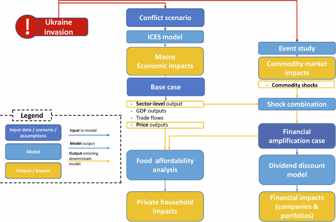
Blue elements depict the main cases, the base case, and the finance amplification case, turquoise the models/analyses, and yellow the outputs, i.e. impacts.

Full size image

War scenario

We define a stylized war scenario to ground our analysis and to mimic the factual situation and consequences from the point of the invasion in 2022. The scenario includes a series of plausible but severe commerce-related sanctioning measures (such as restrictions on specific sectors such as agricultural products, fertilizers, and energy products) and production capacity disruptions simulating international measures against the Russian invasion of Ukraine and the destructive effects of the war itself, respectively. This scenario is the reference to evaluate the macroeconomic effects of the invasion. Please note that our scenario was designed based on what seemed plausible at the time before the actual commerce-related measures came into force. This scenario does not incorporate aspects that emerged after a year of war duration. It does not account for the bypassing of commerce-related measures (assuming their full enforcement) or the ramp-up of the Russian war industry. The scenario assumes a very strong shock on Ukrainian production and exports, in part because it does not factor in mitigating developments such as international negotiations. For instance, it does not include the effects of the Black Sea Grain Initiative, which helped to alleviate some of the export disruptions. A detailed specification is shown in Table 1.

The input shocks reported in Table 1 are imposed in the ICES model in two ways: (i) changes in stocks of primary productive factors (assumptions on capacity disruption), (ii) endogenous changes in export taxes to induce the targeted reduction in real exports (assumptions on commerce-related measures and trade disruption). While capacity disruption shocks are imposed at the regional level, shocks on trade are sector-specific and pairwise-specific for trading partners. For a detailed description of how these assumptions work in the ICES model to move from a pre-shock to a post-shock equilibrium see Supplementary Information subsection 4.1.

Macroeconomic model

The intertemporal computable equilibrium system (ICES) Model is a standard neoclassical recursive-dynamic general equilibrium model based on the GTAP-E model⁷⁹. The model uses the Global Trade Analysis Project (GTAP) database version 10a⁸⁰ for 2014, which provides a series of interlinked social accounting matrices (SAMs), giving a comprehensive account of payments among productive sectors and final uses in each country. For this analysis, we enrich the model with the GTAP multi-regional input–output (MRIO) database⁸¹, which allows for more detailed tracking of international trade flows among countries. The ICES model was set up according to the regional and sectoral aggregation reported in Supplementary Tables IX and VII, respectively. For each time period ICES gives a comprehensive account of payments among productive sectors (i.e. activities employing factors of production and intermediate inputs to produce), consumption (private and public) and investment, trade (foreign and domestic), tax payments (among private household, government and the rest of the World), and factor income distribution (a graphical exposition of the circular flow of income in ICES is shown in Supplementary Fig. 17). Agents are rational such that they act according to price/quantity signals received from the economic system and they do not form expectations about future dynamics. Moreover, in each period, the model describes the constraints under which the economy acts (budget constraints of institutions, macro balances; constraints in the factors and commodities markets). For a more detailed description of the main characteristics of the ICES model, see Supplementary Information section 4.1. To portray a short/medium-run baseline for the macroeconomic assessment of the war scenario as described in Table 1 we use 2020 as a proxy reference for the year 2022 without war and make the following assumptions and adjustments. Firstly, to better reflect the behavior of fossil fuel markets in the medium-run term, we introduce the supply elasticity parameters following Beckman et al.⁸² who validated those values. Secondly, to simulate short-term responses with an additional major rigidity of international trade due to the outset of the war, we reduced the original elasticities that govern international trade in the model. The scenario was designed at the beginning of the war, and it might differ from what effectively happened. To check for the robustness of results and identify key macroeconomic dynamics we also provide two additional scenarios within a sensitivity analysis, details can be found in Supplementary Information Section 1.

Financial model

The financial model used in this study stacks multiple components. First, an event study analysis to quantify abnormal returns. Second, the calculation of commodity-level shocks. Third, the analysis of changes in companies’ equity valuation. Fourth, the propagation of equity shocks in investors’ portfolios. The next paragraphs describe each step.

Event study analysis

We collect data on daily close prices for 29 commodity futures between 01.01.2018 and 21.12.2022 from Refinitiv Eikon⁵⁸. We use continuation futures, which are automatically rolled at the end of the month by Refinitiv. We also collect information on 1 commodity index and 9 commodity spot prices. The descriptions and summary statistics for all contracts are reported in Tables X and XI in the Supplementary Information. On trading days, we interpolate up to 5 missing prices. We compute log returns for the whole time series. We define the “normal” conditions for the event study as the window −125 to −6 days from the start of the invasion, 24.02.2022. The “event” window covers −5 to +5 days around the event date. We compute a market model based on the Bloomberg Commodity Index (ticker: BCOM) and estimate abnormal returns (also called excess returns) around event day as

where AR_i,t is the abnormal return for future i on day t, R_i,t the observed return for future i on day t, ({hat{R}}_{i,t}=({alpha }_{i}+{beta }_{i}{R}_{{ {m}},t})) the return predicted by the market model for future i on day t, and R_m,t the market return, in this case, the Bloomberg Commodity Index, on day t. α_i is the regression intercept and β_i the regression slope. Abnormal returns can be cumulated over the event window to derive the cumulative abnormal returns (CAR):

where t₁ is the beginning of the time window and t₂ is the end of the time window (respectively, −5 and +5 days from the event). We compute the CAR over the event window and test for significance using a 2-tailed parametric t-test.

Commodity shocks

We define the abnormal reaction in the market as the CAR over the [−5, +5] days event window. This represents the input commodity shock. The shock propagates through the market based on the ICES model cost structure data. We assume that companies relying more on a certain input (e.g., gas) whose return is unexpectedly high will face higher costs, thus worsening their profitability and reducing the value of their equity. We first map commodity futures to ICES sectors and regions to represent initial shocks:

where ({varphi }_{r,s}^{{rm {I}}}) is the initial (I) shock on region r and sector s, measured as the CAR between t₁ and t₂ for commodity i which is mapped to sector s and region r (i → (s, r)). Assuming investors know the cost structure of sectors, the initial shock propagates to those sectors that are not affected by it in the first place. These sectors then suffer a direct shock:

where ({k}_{r,o}^{s}) is the share of input the sector s uses from sector o in region r, N_s is the number of sectors, ({varphi }_{r,o}^{{rm {I}}}) is the initial shock on sector o, and ({varphi }_{r,s}^{{rm {I}}}) is the initial shock on sector s. Thus, the direct shock represents the difference between the initial shocks on a given sector, weighted by their relevance in its production process, and the initial shock on that sector. In a simplified example, an electricity producer using only gas as input will experience a negative initial shock on gas (({varphi }_{r,o}^{{rm {I}}})) as the cost increases, a positive shock on its output (({varphi }_{r,s}^{{rm {I}}})) as electricity prices rise, and the difference would be the direct shock (({varphi }_{r,s}^{{rm {d}}})). Thus, the commodity shock captures both the direct initial overreaction and its first-round propagation in the economy. In this study, we propagate initial shocks from energy commodities only, as other commodities either do not exhibit significant abnormal returns (e.g., gold) or are of little relevance for equity markets (e.g., wheat).

Financial valuation model

We use a dividend discount model (DDM) (building on refs. ^83,84,85) to estimate the value of equity given dividends⁸⁶ and assumptions on the discount rate r and the long-run dividend growth rate g_L. For the purpose of this study, we assume g_L = 2.5% and r = 5%. We use a two-stage DDM to estimate the value V₀ of equity at time 0 (for a complete list of assumptions, see Supplementary Tables IV–VII, IX):

where t is time in years, D_t is the dividend at time t, n is the last year of valuation. This represents the estimate of the equity value of a given company, considering the dividends as estimated before the invasion of Ukraine. To estimate the equity value after the invasion, we assume that dividends are reduced by a shock γ which depends on the sector and region of operation of the company:

furthermore, we assume that γ_n = 0, and that γ_t linearly declines in time from t₀ to n. Thus, we are assuming that the shock is temporary and mostly affects short-term dividends. We consider two effects to compute γ_t: an output effect and a price effect. The output effect depends on the change in output computed by the ICES model for a given sector and region (denoted by η_r,s). Thus, we assume that the dividends of companies in sectors that contract because of the war are going to be lower. For our base case, only the output effect plays out in the financial models. The price effect depends on the increase in prices as described by φ above, computed using the event study analysis. Thus, we assume that the dividends of companies whose input prices increase are going to be reduced. We combine the output and price effects to derive the shock on equity in our finance amplification case:

Finally, we can compute the shocked equity value ({tilde{V}}_{0}) by applying Eq. (5) with shocked dividends from Eq. (6). This is the equity value considering the consequences on companies from the invasion:

Combining Eqs. (5) and (8) we can obtain the loss (gain) on a given equity stock stemming from the adjustment in valuation:

Equation (9) is applied to all companies with at least two data points available for earnings per share (EPS) and, thus dividends. For stocks paying no dividend, or with no dividend data, or where the values resulting from Eqs. (5) or (8) are negative, we revert to direct shocks, i.e.

Portfolio impacts

We collect a database of equity portfolios of European investors as of June 2020 from Refinitiv Eikon (see Supplementary Information subsection 4.3.5). Using the monetary value of each position, we can derive the total portfolio value and the portfolio share invested in each security. Then, for each portfolio, we can compute the portfolio-level shocks as the weighted average of company-level shocks:

where m indexes securities, ζ_m is the company-level shock as per Eq. (9) or Eq. (10), w_m is the weight of security m in the portfolio, and ζ^P is the portfolio-level shock. We compute portfolio-level loss and gain trends, considering only investors with at least 30 positions and 5% of invested shares in a certain macro-sector or region to remove noise.

Food affordability

Food affordability is determined as the absolute number of people who cannot afford specific diets anymore due to the increased prices of food commodities in two cases: the base case and the finance amplification case. We follow the approach of Herforth et al. and the FAO^87,88 and use income levels in countries⁶⁴ or individuals⁶³ by the World Bank to derive the available household budgets for food. To determine food affordability, these budgets are compared to inflation-adjusted costs of two reference diets: a calorie-sufficient diet and a healthy diet. The basic costs of a calorie sufficient and healthy diet are provided by World Bank⁸⁹ for 186 nations at retail price data of 2017 (expressed in 2017 purchasing power parity (PPP) dollars). We consider these diets relevant as ensuring calorie sufficiency implies that individuals are not suffering from hunger. Further, a healthy diet refers to the definition of food security by the Committee on World Food Security as a state when “all people at all times have physical and economic access to sufficient, safe, and nutritious food to meet their dietary needs and food preferences for an active and healthy life”⁹⁰. Thus, the affordability of a healthy diet also gives us an estimate of how many people are able to get all the nutrients required, which is especially important for children and women of reproductive age. For the number of affected people, we provide lower and upper-bound estimates. The lower bound estimate is calculated assuming that 63 percent of the monetary household budget available is spent on food. Upper bound estimates adjust the share of the budget that must be spent on non-food items (e.g. rents) and are based on average food expenditure shares with respect to the World Bank’s classification of income levels in countries⁶⁴. Here, food budgets are, on average, 15%, 28%, 42%, and 50% of the individual income groups in high-, upper-middle-, lower-middle- and low-income countries, respectively⁶⁴. The cost of the diets is defined as the lowest-cost set of items available at each time and place that would meet requirements for each food group specified in Food Based Dietary Guidelines⁹¹. The cost of healthy diets is, on average, nearly five times as expensive as the cost of energy-sufficient diets. The diet costs are inflation-adjusted by using the global mean for the share of costs for the two diets, as cost contribution does not vary much across income country classes. On a global mean, starchy staples (c_c) account for 12% of a healthy diet’s cost, while protein-rich foods and dairy (c_a), as well as fruits, vegetables, and fats (c_v) each constitute 44%. To compute the inflation for the diets we take the mean price increase from the base case given by the ICES model or the mean price increase (in percent) of the finance amplification case given by the event study of starchy staples i_c, of protein-rich foods i_a, and of i_v vegetables, fruits, and fats (see exact mapping from commodities to composition in Supplementary Table XII). Thus, the inflation-adjusted costs are given by: C = ∑_{x∈{c, a, v}}c_x (1 + i_x). The approach for the calorie-sufficient diet is analogous but for adapted shares of starchy staples, protein-rich foods, and fruits and vegetables (see also Supplementary Table XII).