Causation versus prediction in travel mode choice modeling

Introduction
Modeling is central to transport planning. Yet, choosing the appropriate model for individual applications is challenging. In particular, the importance of the modeling purpose must be emphasized as different modeling approaches serve different purposes. As Shmuell1 explains, modeling approaches can be broadly grouped in three categories: explanatory modeling, predictive modeling, and descriptive modeling. Explanatory modeling tests causal hypotheses about some theoretical constructs using statistical models on data. Predictive modeling predicts new or future observations by using statistical models or data mining algorithms on data. Descriptive modeling summarizes or represents a data structure in a compact manner, with the causal theory being either absent or implicit. This article focuses on the first two modeling approaches – explanatory and predictive. Explanatory or causal modeling (as we refer to it throughout this article) differs from predictive modeling, especially when dealing with a finite quantity of real data. In other words, the optimal model for prediction purposes differs from the one estimated to explore the underlying mechanisms2. Transport researchers must choose between causation and prediction when developing a model3, but the line between causal and predictive modeling has been blurry in the travel mode choice community.
Since its earliest applications in cities like Chicago and Detroit several decades ago4, mode choice modeling has become a classic problem in transport5,6. Several methods have been proposed in the literature to perform mode choice modeling. Discrete choice models based on random utility theory are likely the most extensively used models for mode choice modeling7. Discrete choice models predict the choice between two or more available alternates that are mutually exclusive and collectively exhaustive8. Random utility models assume that the decision maker selects the alternative that offers the highest utility9. Examples of discrete choice models based on random utility theory include MNL and probit models. Many studies have used these models to study mode choice10,11,12. In recent years, ML has been applied to several mode choice modeling problems. Some ML algorithms that have been used to model mode choice include random forest13, support vector machines14, extreme gradient boosting15, and artificial neural networks (ANNs)10,16. Several studies have compared the performances of ML algorithms for mode choice prediction, albeit with no final consensus16,17,18,19,20, while some others found ANNs to perform best17,18. ANNs have been praised for their superior prediction performance and the ability to capture non-linear relations10,17,21.
Statistical models, like MNL, offer good interpretability and are often used to understand the underlying mechanism as if they were causal models, but they are not. Since they are based on correlations, their findings cannot be interpreted in terms of causality. Similarly, despite all the advantages that ML algorithms offer, they are appropriate only for prediction or correlation-based interpretation. These techniques have not been able to provide causal understanding. Regardless, there has been a keen interest in unraveling causality in mode choice behavior22,23,24,25,26,27,28. One of the methods that researchers have used to estimate causal models for mode choice is structural equation models (SEM)22,28. SEMs are considered to be causal models, but they are generally used as confirmatory tools, not exploratory29. The accuracy of their causal findings depends upon the accuracy of the causal assumptions made by the researchers29. SEMs take these causal assumptions as their inputs and test their suitability on data. They are not useful in extracting causal relations directly from data30,31. It is a major limitation of most of the causal models used for mode choice that these studies rely upon the hypothetical causal structures assumed by researchers22,25,27,28. As of this writing, only a handful of studies have derived an underlying causal network behind mode choice decision making directly from data31,32,33,34. These studies have applied different algorithms to study causality.
Understanding the fundamental differences between causal and predictive modeling is important. As explained in Shmuell1, let us hypothesize that χ causes ϒ through a function Ϝ such that ϒ = Ϝ(χ). Measurable variables X and Y, and a function f are the operationalizations of χ, ϒ, and Ϝ, respectively, such that E(Y) = f(X). In causal modeling, the variables X and Y are used to estimate f with the goal of matching f to Ϝ. In contrast, predictive modeling is interested in X and Y directly, and f is used to predict the new values of Y, not to predict ϒ. It is even possible that a function other than the estimated f(X) (denoted as (hat{f}(X))) may be preferable for prediction, despite the causal relation being ϒ = Ϝ(χ). There are other major differences between causal and predictive modeling. Namely, causal modeling is based on causation, while predictive modeling is based on associations (or correlations). Causal modeling is retrospective, while predictive modeling is prospective1. The accuracy of predictive modeling is easier to test and observe, while the results from causal modeling can never be fully confirmed1.
While the literature on correlation-based modeling or predictive modeling of mode choice is abundant, the literature on causal modeling of mode choice is scant. An important reason for this is that determining causality from observed data is complicated. To know whether a certain variable causes another variable or not, we must compare the outcomes with versus without the presence of that variable. In the real world, only one of the outcomes can be observed. This leads to the fundamental problem of causal inference35. To circumvent the major challenges associated with determining causality, researchers have developed specialized causal models. The two major techniques to study causality are causal discovery and causal inference. Causal discovery is the process of extracting causal relationships directly from observational data, while causal inference is the process of estimating the quantitative causal effects from a change of a certain variable (cause) over an outcome of interest (effect)36. Despite being in their infancy, these emerging methods have found applications in several disciplines.
The goal of this study is threefold: (a) to develop causal models for mode choice using causal discovery and inference; (b) to compare the performance of a causal model with a prediction model; and (3) to highlight the key differences in the analysis from each technique. Data from three Chicago neighborhoods, i.e., North Side, West Side, and South Side, are used to compare the performance of the models. Instead of looking at Chicago as a whole, we decided to divide the city into three neighborhoods because we know people’s decision-making processes are different in the three neighborhoods and wanted to explore to what extent the models could capture these differences.
For causal modeling, travel data and some basic domain knowledge (explained later) are provided as inputs to the Peter-Clark (PC) algorithm (a conventional and simple causal discovery algorithm described in the Methods section). The causal discovery algorithm uses data to produce causal structural graphs which are a visual representation of the causal network among the study variables. Then, these causal structural graphs are used in a causal inference method – namely Double Machine Learning (DML) – to estimate causal effects. For predictive modeling, ANN models are developed in a traditional way using mode choice as the target variables and the other variables are explanatory variables. Figure 1 depicts the two approaches for mode choice modeling.

Statistical and machine learning techniques have been extensively used to develop prediction mode choice models from travel data. The combination of causal discovery and causal inference provides a means to better capture the causal relationships between the variables and their causal effects on mode choice. Causal discovery algorithms use travel data and some basic (minimum) domain knowledge as input to produce causal structural graphs which are then used as an input to a causal inference method to estimate the causal effects.
Overall, our study contributes to the travel mode choice modeling literature by assessing the potential of new causal models and by comparing their value with more traditionally studied prediction models. By doing so, we wish to bring attention to causal discovery, which has been overlooked by the travel model choice modeling community. Additionally, this is the first study to use the Double Machine Learning (DML) causal inference method to study mode choice.
Results
Causal Models
Figure 2 shows the causal graphs obtained from the PC (Peter Clark) causal discovery algorithm for all three neighborhoods of Chicago. There was one edge in each of the three graphs that the algorithm was not able to direct. These were between trip purpose and trip distance (work_prup – distance_x) in the North Side and South Side, and between household size and annual household income (hhsize – hhinc) in the West Side. These were oriented as trip purpose to trip distance (work_prup → distance_x) and household size to annual household income (hhsize → hhinc) based on domain knowledge. Table 1 shows the total causal effects obtained from DML. These values are the average treatment effects (ATE), meaning the average difference in the pair of potential outcomes averaged over the entire dataset. These causal effects can be interpreted as the average change in outcome caused by the treatment. A positive value suggests an increase in outcome, while a negative value suggests a decrease.
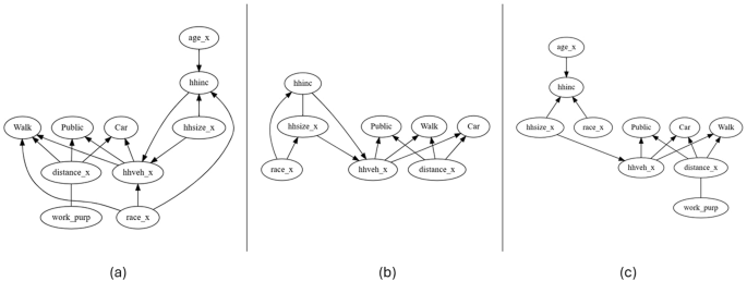
Causal graphs for the (a) North Side, (b) West Side, and (c) South Side of Chicago. The causal graphs present a visual representation of the flow of causality. The causal connections are depicted by directed edges such that X is the direct cause of Y in X → Y. Owning a vehicle (hhveh_x) and trip distance (distance_x) are the direct causes of choosing a travel mode (Walk, Public transit, and Car) in all three neighborhoods. Unlike the North and West, the South Side also has race as a direct cause of choosing to walk.
The causal graphs present a visual representation of the flow of causality over the decision variables and shed light on mode choice decision making. Figure 2 shows that vehicle ownership and trip distance are the two direct causes of choosing any mode in all three neighborhoods. It is only in the South Side that race is also a direct cause of walking (discussed below). The direct causes of vehicle ownership are household size (in all three neighborhoods), household income (in the West Side and South Side), and race (in the South Side). The direct cause of trip distance, in the North Side and South Side, is work related purpose of trip.
The total causal effects on mode choice also provide meaningful insights. In the North Side, the causal impact on choosing car comes from vehicle ownership (0.41), household size (0.09), trip distance (0.08), and work-related purpose of trip (-0.04). Further, the causal impact on choosing public transit comes from vehicle ownership (-0.31), work-related purpose of trip (0.13), trip distance (0.10), and household size (-0.06). Finally, the causal impact on choosing to walk comes from trip distance (-0.17), vehicle ownership (-0.10), work-related purpose of trip (-0.09), and household size (-0.06).
In the West Side, the causal impact on choosing car comes from vehicle ownership (0.49), trip distance (0.08), white race (-0.06), and household income (0.02). Further, the causal impact on choosing public transit comes from vehicle ownership (-0.38), trip distance (0.07), white race (0.06), and household income (-0.02). Finally, the causal impact on choosing to walk comes from trip distance (-0.16), vehicle ownership (-0.11), white race (-0.04), household size (-0.03), and household income (0.01).
In the South Side, the causal effects on mode choice are spread out over several causes. All the variables that were suspected to have a causal effect on mode choice (household income, white race, vehicle ownership, household size, age, trip distance, and work-related trip purpose) had a causal effect on all three modes. Although vehicle ownership stands out among all other variables due to its high causal impact on choosing a car and public transit (0.56 and -0.47 respectively).
It is interesting to note that race has no causal effects on mode choice in the North Side, while it does on every mode in the West Side and the South Side. Race is also a direct cause of household income, and it has a very high causal effect on household income which is even more pronounced in the West Side and the South Side. More generally, the inclusion of race as an explanatory variable can be controversial and is discussed below. Another key finding is that household size was found to be a direct cause of owning vehicle in all three neighborhoods.
Prediction Models
When applied to each neighborhood, the ANN models achieved an accuracy of 75.46%, 74.68%, and 72.50% for the North Side, the West Side, and the South Side, respectively.
Figure 3 shows the SHAP values of the different variables on the model output. These values are based on prediction and are the average impact of the variables on model prediction. For each neighborhood, the variables are ordered based on their magnitude of influence (with the largest at the top). In all three neighborhoods, the most important variables are trip distance and vehicle ownership. Notably, race has a more significant role in the South Side than in the North and West. The variable importance also varies with mode type. In all neighborhoods, trip distance has the largest influence on walking. Vehicle ownership has the highest impact on choosing the car mode in the North Side and South Side while, for the West Side, it is distance. Household size plays an important role in car choice in the North Side while, in the West and South, it is household income. Further, the biggest impact on choosing public transit is from trip distance in the North Side and West Side and vehicle ownership in the South Side. However, we note that for all three neighborhoods, the models performed worse for public transport than car and walk mode. This can be indicative of the fact that demographic attributes/ user-specific variables do not always behave consistently in predicting mode choice for public transport37.
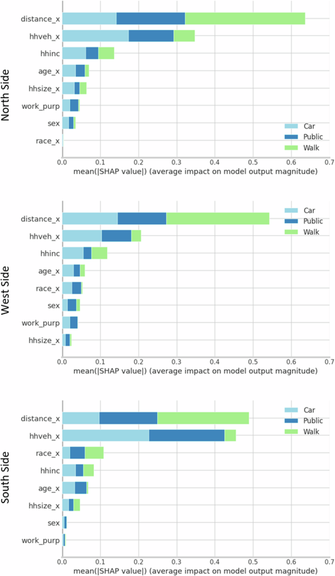
The SHAP values quantify the average impact of each variable on model prediction such that the greater the SHAP value the greater the variable’s influence on prediction. In all three neighborhoods, the most important variables are trip distance and vehicle ownership.
Combined Insights
The results from the causal and prediction models highlight the role of trip distance and vehicle ownership on mode choice. For each mode in the three neighborhoods, these two variables emerge as direct causes and are among the variables with the highest SHAP values. Beyond similarities, the results highlight the difference in mode choice behavior across the neighborhoods. For example, race was found to have causal effects on mode choice in the West Side and South Side but not in the North Side. Similarly, household size is the direct cause of household vehicle ownership in the North Side. Household income in the West Side, and household income as well as race in the South Side are also direct causes of vehicle ownership. These differences in mode choice behavior reflect, in part, differences in the characteristics of the neighborhoods themselves as discussed in the Data Preparation section. Based on the 2020 census38, the North Side enjoys a much higher median household income and a much lower registered crime per person ($86,359 and 116.7) compared to the West Side ($63,466 and 189.5) and the South Side ($46,792 and 150.2). Additionally, the North Side has a smaller share of Black and Hispanic populations (36.2%) compared to the West Side and South Side (~80%)38. Several of these differences are systemic and have led to uneven infrastructure development across the city. Exploring deeper ties between travel behavior and neighborhood characteristics is beyond the scope of this study.
Discussion
In this section, we comment on the two modeling approaches for mode choice modeling:
-
I.
Causal modeling and predictive modeling are two distinct modeling approaches. As mentioned earlier, the goal of causal modeling is to understand the causal relations while that of predictive modeling is to predict the future1. Both are suitable for their own specific applications. When selecting between the two, the modeler needs to contemplate the purpose of modeling. Travel mode choice modeling may be one of the unique avenues where both approaches can find their applications. Causal modeling could be helpful for knowing where to intervene to bring a mode shift, while predictive modeling could aid in estimating the need for infrastructure in the future.
-
II.
Results from the causal model and the prediction model show some similarities. Despite their fundamental differences, the results from both approaches exhibit some notable similarities. For example, the causal models suggest that trip distance and vehicle ownership are the direct causes of choosing any mode in all neighborhoods (Fig. 2). These two variables also have the highest SHAP values in all neighborhoods (Fig. 3). Similarly, causal models found race to have no causal effect on choosing any mode in the North Side, unlike the other two neighborhoods. This is reflected in the SHAP values where race is at the bottom of the list in the North Side but is important in the West and South. It is unclear whether these similarities are only a coincidence or if they point to something meaningful about the two approaches and/or data. Further analysis is needed on this point.
-
III.
Causal models are built on some noteworthy assumptions. The causal discovery and inference techniques are based on certain assumptions. For example, the methods used in this study, the PC algorithm and DML (with a Lasso Linear Regression model to estimate residuals), assume the absence of any unobserved confounders and linear variation in causal effects, respectively. Therefore, the true causal graph for mode choice may have more variables than those shown in Fig. 2 and/or may have non-linear causal effects. Additionally, the variables in a causal model may be a proxy. In particular, the variable race is hypothesized to be a proxy for complex social, political, economic, and cultural factors as explained in Chauhan et al. 31. Researchers must be careful in picking the causal techniques and be mindful of their assumptions and the data used in the study.
-
IV.
Causal models can guide interventions, but prediction models may not. Despite the few assumptions and limitations associated with the causal discovery and inference techniques, they are truly causal in nature. As such, they can extract the causal structure and estimate the causal effect from observed data. Being based on causation, they could suggest where to (and where not to) intervene to bring about a desired change. For example, intervening on any variable that has zero causal effect on mode choice will not lead to a change in the selection of that mode. The SHAP values from the prediction models cannot guide us about interventions since these values are based on the impact of a variable on prediction, which does not necessarily indicate a causal relation between the variable and the predicted variable. For instance, the variable sex does not even appear in the causal graph; however, it still has a non-negligible SHAP value.
-
V.
Both causal and prediction models may be capturing regional variations in travel behavior. Firstly, the causal graphs and SHAP values have remained moderately similar across the neighborhoods. This makes sense since all three datasets are from the same city with some geographic variation in travel behavior. This may also be indicative of the robustness of both models. Secondly, models show that walking in the South Side is different from the North Side. The causal graph suggests that race is a direct cause of walking in the South Side (unlike anywhere else). The SHAP values of race for predicting walking is much higher in the South Side as well. Here again, race may be a proxy for complex factors, possibly around safety.
-
VI.
Causal models have under-explored potential in mode choice modeling. Mode choice modeling has been mostly conducted through predictive modeling. Causal discovery and inference techniques have rarely been applied and show much promise. Causal modeling could create new avenues to study mode choice and reshape our understanding of the mode choice behavior.
Conclusion, Limitations, and Future Work
As of this writing, travel mode choice studies have been dominated by correlation-based models, including both statistical and ML models. Studies on causal modeling of mode choice remain limited.
New causal discovery and inference techniques allow for the estimation of data-driven causal models. A combination of the PC algorithm and DML is used in this article to estimate causal relationships to model mode choice in three Chicago neighborhoods. The result is a graphical representation of the flow of causality in the decision-making process as well as the quantitative estimation of the causal effects among the variables. We find that the two direct causes of choosing any mode (car, public transit, or walk) in any of the three neighborhoods are trip distance and vehicle ownership. Race was also found to be a direct cause of walking in the South Side. The estimated causal effects present the strength of any direct or indirect causal effects in the mode choice process.
For comparison, three ANN models were also estimated and performed relatively well (over 70% accuracy). The SHAP values from these models provided insights into the importance of each variable. Even though causal modeling and predictive modeling are fundamentally different, they found many similar results. Both models seem to capture some geographic variation in travel behavior in Chicago. Overall, both modeling approaches have their usefulness in mode choice modeling.
The study found great value in causal discovery and inference to model travel mode choice. Causal modeling reveals the underlying causal relations from the data and can advance our understanding of mode choice behavior. Despite their usefulness, causal models also have limitations. These limitations largely stem from the choice of the causal discovery algorithm and causal inference method. Some of the most important shortcomings of the causal model used here (i.e., PC algorithm and DML with Lasso linear regression) are their inability to account for any observed (or hidden) confounder, non-linearity, and cyclicity. Causal relations in the real world may be more nuanced and complex than the ones found in this study. Here, we used the PC algorithm since it outputs easy to read and interpret causal graphs, but readers are encouraged to seek other algorithms as well. In another study31, we tested four algorithms: PC, Fast Causal Inference, Fast Greedy Equivalence Search, and Direct Linear Non-Gaussian Acyclic Models. We found that the latter performed best; it also generated much more complex, less-easily interpretable causal graphs.
Overall, causal modeling is a developing field. More sophisticated methods are being developed to overcome existing limitations. More research is also needed to realize the full potential of causal models for travel mode choice modeling, in particular about (a) the choice of causal discovery and inference techniques most suitable for mode choice studies, (b) the analysis of causal model results developed on different datasets with more variables, and (c) the use of causal models to make predictions and to compare the accuracy with prediction models.
Methods
Data Preparation
To compare the performance of causal and prediction models, this study uses data collected by My Daily Travel survey conducted by the Chicago Metropolitan Agency for Planning (CMAP)39. The survey was conducted in northeastern Illinois (including the city of Chicago) and was completed in 2019. The survey asked the respondents about their travel behavior and mode choices. Since the travel behavior within the city might be quite different from that in surrounding areas, we only focused on the data collected from Chicago. Based on our domain knowledge and available literature, we filtered out several variables that might be relevant to mode choice. These variables can be categorized into three categories: socio-demographic information, trip characteristics, and mode choice. Table 2 lists the study variables and references selected studies that identify variables influencing mode choice.
The survey data were first cleaned. Any invalid or unknown responses were removed. These include responses like ‘not ascertained’, ‘I don’t know’, ‘I prefer not to answer’, and appropriate skip. Only private vehicles (car), public transit, and walking modes were studied since these are the most used travel modes, accounting for about 90% of the combined share of all trips in Chicago39. The variables were converted to ordinal or binary variables before modeling. To have multiple datasets to study the model performances and to capture the regional variation in travel behavior, the data were split into three datasets, each corresponding to three Chicago neighborhoods.
Dividing the city into these macro clusters recognizes the unique characteristics and challenges faced by different regions. This is particularly important for Chicago since it is defined as a “city of neighborhoods” with stark socioeconomic disparities critically fluctuating from neighborhood to neighborhood due to the historical context of neoliberal governance, with exclusion, segregation, and redlining hidden under the policies40. These disparities often align with geographical locations, creating distinct pockets of affluence as well as disadvantages and disinvested areas41,42. To address these issues, splitting Chicago into neighborhoods is important for our analysis as well as for policy recommendations regarding the allocation of resources, infrastructure development, and public services.
We used Census data38 at the standard division of the level of 77 community areas, which the city of Chicago uses to collect data43,44. These areas were grouped by socio-economical similarities into three broader clusters, namely North Side, West Side, and South Side. At this geographical level, each of these neighborhoods represents their unique socioeconomic dynamics. The North Side and the central part (including Loop – central business district) are predominantly characterized by higher-income neighborhoods with significant White and Asian populations and robust commercial and business-centric nature. The South Side experiences greater poverty rates, higher unemployment, transit and food deserts, and a larger Black population. Finally, the West Side is somewhat similar to the South Side in some characteristics, including low median income, massive industrial lots, higher poverty rates, and limited economic opportunities. The West Side has a Black and Hispanic population proportion intermediate between the two other neighborhoods. Figure 4 shows the locations of the three neighborhoods on the map of Chicago.
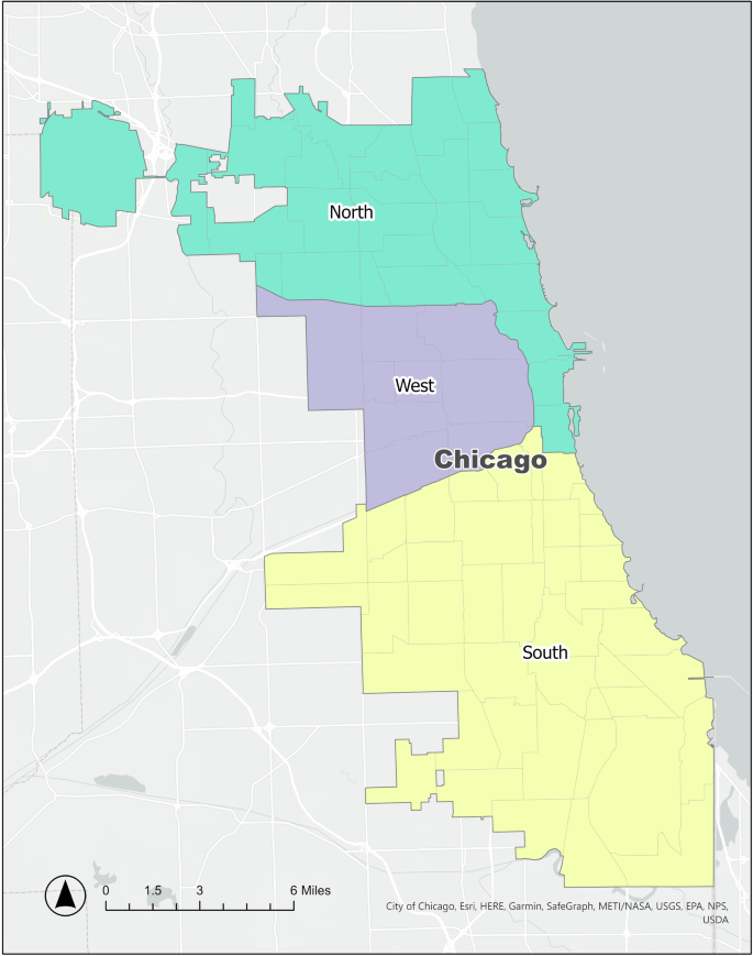
Based on socio-economic similarities, the city of Chicago is divided into three neighborhoods: the North Side, the West Side, and the South Side. The North Side, including the central business district, is predominantly characterized by higher incomes, significant White and Asian populations, and a strong commercial/business sector. In contrast, the South Side has higher poverty rates, higher unemployment, transit and food deserts, and a larger Black population. The West Side is somewhat similar to the South Side with low median income, massive industrial lots, higher poverty rates, and limited economic opportunities, but with a Black and Hispanic population proportions intermediate between the two other neighborhoods.
Basic Concepts on Causal Discovery
A directed acyclic graph (DAG) is denoted by G = (V, E) where V are vertices and E are edges45. DAGs are directed, meaning the edges have a direction, for example V1 → V2. The node where an edge begins is called the parent node (like V1 in V1 → V2 which can be denoted as Pa(V2)), while the node where the edge points is called the child node (like V2 in V1 → V2). A path in a graph is defined as a sequence of adjacent edges. In a DAG, all the nodes preceding a node in a directed path are called its ancestors, while all the nodes succeeding it in a directed path are called its descendants. The Markov condition states that any node X (X Î V) is independent of its non-descendant nodes conditioned on its parent nodes (Pa(X) ⊂ V)45. Bayesian networks are used as a means to perform causal discovery and inference45. For a given set of variables V, a Bayesian network could represent the joint probability distribution P(V) through a DAG, assuming the Markov condition applies45. A Bayesian network is considered a causal Bayesian network when its structure is considered causal, such that V1 is considered a direct cause of V2 in V1 → V245.
A path V1, …, Vn in a DAG is said to be blocked by a set of nodes Z (not consisting of V1 or Vn) if: (a) there is a node Vk in the path that is a non-collider (i.e., it is either Vk-1 → Vk → Vk+1 or Vk-1 ← Vk ← Vk+1 or Vk-1 ← Vk → Vk+1) and Vk є Z, or (b) there is a node Vk in the path that is a collider (i.e., Vk-1 → Vk ← Vk+1) and neither Vk nor its descendants belong to Z36. If in a DAG (G), a set of nodes Z blocks all the paths between two sets of nodes A and B, given that A, B, and Z are pairwise disjoint, then A and B are said to be d-separated by Z. This can be mathematically denoted as (A{perp }_{G}{B|; Z})36. The global Markovian condition is satisfied in a DAG if for every pairwise disjoint (A,{B},{Z}subseteq V), (A{perp }_{G}{B|; Z}) implies  36.
36.
Two more relevant concepts need to be discussed before moving on to the causal discovery algorithms. These are the assumptions of faithfulness and causal sufficiency. The faithfulness assumption is the same as the global Markovian condition but reversed, such that  implies ({A}{perp }_{G}{B|; Z})36. As per the causal sufficiency assumption, all the common causes of any pair of variables in the observed data are also observed in the dataset36.
Peter-Clark (PC) Algorithm
There are several causal discovery algorithms suggested in the literature36,46. In this article, we have chosen to use one of the most popular causal discovery algorithms, the PC algorithm47. Note that finding the most suitable algorithm for mode choice modeling is beyond the scope of this article. Please refer to Chauhan et al. 31 for more on the topic. The PC algorithm uses conditional independence to extract causal relationships from observed data. With the assumptions of causal Markov, faithfulness, and no latent confounders, the PC algorithm suggests that two variables are directly causally related if and only if there exists no subsets of remaining variables conditioning on which the two variables are independent46,47. As explained by Glymour et al. 46., the PC algorithm involves the following steps in sequence:
-
The algorithm starts by assuming a complete undirect graph where every variable has an edge connecting to every other variable.
-
The edge between a pair of variables (say A and B) is eliminated if they are found to be conditionally independent i.e.,
 .
. -
For each pair of variables (say A and B) that have an edge between them, the edge is eliminated if
 for any variable C that has an edge connected to either A or B.
 -
For each pair of variables (say A and B) that have an edge between them, the edge is eliminated if
 for any pair of variables {C, D} that have edges both connected to either A or B. Continue testing the independencies conditioned on subsets of variables of increasing size until there are no more left.
 -
For each triple (say A, B, and C) with an undirected edge between A and B and between B and C but not between A and C (i.e., A – B – C), be oriented to A → B ← C if B was not in the set conditioning on which A and C became independent.
-
For each triple (say A, B, and C) with a directed edge between A and B and undirected edge B and C but none between A and C (i.e., A → B – C), B – C should be oriented to B → C as per orientation propagation.
There may be other orientation propagation rules as well46. An edge may remain undirected if none of the orientation rules of the PC algorithm apply46. The Pycausal Python library was used to run the PC algorithm in this study48.
Double Machine Learning (DML)
There are several methods to estimate causal effects. In this study, we adopt a Double Machine Learning (DML) causal inference method49. Assume a treatment variable T that has a causal effect on an outcome variable O, and a covariate variable Z that causes both T and O, DML performs three main steps to estimate the causal effect of T on O: (a) two ML models are estimated – first to predict O by Z and second to predict T by Z; (b) the residuals from both the models are computed; (c) the residual from the model predicting O by Z is regressed on the residual from the model predicting T by Z49. Please refer to Chernozhukov49 for details.
In this study, DML involves two Gradient Boosting Regression models to model the outcome and the treatment, and a Lasso Linear Regression model to estimate the residuals. The DoWhy Python library50 was used to estimate the causal effects based on the causal graphs obtained from the PC algorithm.
Domain Knowledge
Inputting some domain knowledge into the causal discovery algorithms improves the model results32,51. We added four rules to our algorithm, keeping it to the very minimum so as not to bias the model results:
-
The three mode choice variables (car, public, and walk) cannot cause any other variables. In essence, they become akin to target variables.
-
Gender, race, and age cannot be caused by any variables (i.e., they are considered exogenous). Exploring the causes of gender, race, and age is beyond the scope of this study.
-
Gender and age cannot cause household size. A household usually comprises members of different genders and ages; thus, household size cannot be caused by gender or age.
-
Vehicle ownership cannot cause household size or household income. While the three variables are linked, having a causal relationship between vehicle ownership and household size or income does not make sense.
Artificial Neural Networks (ANNs)
Separate ANN models were developed for the three neighborhoods. The target variables were the three travel modes, and the explanatory variables were the socio-demographic and traffic characteristics variables (Table 2). To develop the ANN models, we had to adopt a pragmatic hyperparameter tuning approach. Since the dataset is relatively small, hyperparameter tuning is performed by combining the data for all three neighborhoods. The data are split into two sets, 80% training and 20% testing with stratified sampling. The training data are further split into three sets, 72% training, 18% validation, and 10% testing to tune the hyperparameters. Keras_tuner is employed to find the best hyperparameters. After trying a different number of layers and neurons with different activation functions, the highest accuracy with the simplest model structure is adopted. In our case, it is as follows: one hidden layer with 28 neurons, the Scaled Exponential Linear Unit (SELU) activation function, and a learning rate of 0.0005. Subsequently, 5-fold cross-validation is performed, and we find that all five models have a consistent accuracy of ~75%. We then train the model one more time on the combined train and validation data, and we test it on the test data to validate the choice of hyperparameters. This step gave us an acceptable accuracy of 74%.
Finally, the model is trained separately on the original 80% training data for each neighborhood and tested one final time on the original testing data for each neighborhood. We note that the testing data was kept separate while tuning the model hyperparameters to avoid data leakage. The accuracies were calculated for each neighborhood using their respective final test sets.
The accuracy of the models was calculated as:
No scaling was applied since all the features are either nominal binary or ordinal categorical. Data were oversampled using Synthetic Minority Over-sampling Technique (SMOTE)52,53 to balance the fewer samples for the public transit and walk modes compared to the car mode. The Keras and SHAP Python libraries were used for the analysis.
SHAP (SHapely Additive exPlanations) values improve the interpretability of ML models19. They quantify the contribution of each feature to the prediction of the model by evaluating the marginal contribution of that feature54,55. The formulation of SHAP value can be expressed as follows56:
where, ({|F|}) is the set of all combinations of features, (S) is a subset of ({|F|}) excluding feature (i), (left|Sright|) is the size of subset S, and ({f}_{Scup {i}}({x}_{Scup {i}})-{f}_{S}({x}_{S})left]right.) is the added value after including feature (i) with (S).


Responses