Changing circulations challenge the sustainability of cold water mass and associated ecosystem under climate change

Climate change induced by greenhouse gases emission from human activities is projected to cause dramatic changes in temperature, circulations, and biogeochemical properties in the ocean^1,2,3,4. The offshore regions and marginal seas are more vulnerable to climate change than the open ocean^5,6,7. The response of these regions to climate change exerts profound influences on human living by impacting fishery, aquaculture, shipping, and tourism, etc.

Bottom cold water mass (BCWM), trapped near the bottom of marginal seas under the strong thermocline in summer, is a widespread phenomenon observed in many shelf seas, such as the Irish Sea, Middle Atlantic Bight, North Sea, Berling Sea and Yellow Sea (YS)^8,9,10,11. It originates from the vertically homogeneous cold water mixed by strong wind and surface heat loss in the previous winter^12,13,14. As reservoirs of cool water and nutrients, the BCWMs serve as the habitat for plankton and cold-water fishes^12,13,14,15. Since nearshore fishing and breeding are approaching their limit, developing aquaculture in the BCWM could be the future solution for the fishery of its surrounding countries^16,17.

Among these BCWM, the Yellow Sea Cold Water Mass (YSCWM) is a unique one, as it resides in one of the most densely populated regions with about 600 million people living in the YS catchment area. It supports various human activities, including fishing, aquaculture and water resource¹⁸. Therefore, understanding the temporal variability and future changes of the YSCWM is crucial for the sustainable development of aquaculture in this region. Based on mooring observations, reanalysis products, and numerical simulations, the interannual variability of the YSCWM is found controlled by local surface wind, buoyancy forcings, and the Yellow Sea Warm Current (YSWC), and modulated by large-scale climatic oscillations, such as El Niño/southern oscillation, Pacific decadal oscillation and Arctic oscillation^14,19,20,21. In terms of long-term changes, an increasing trend of the core temperature of the YSCWM is observed in mooring observations and reanalysis products^22,23,24,25. However, due to the different and limited temporal spans used for analysis, the estimated magnitude of the warming of YSCWM shows the apparent discrepancy between these studies^22,23,24,25. Besides, whether the current long-term changes can represent the response of YSCWM to climate change remains uncertain.

As the warming of the YSCWM may lead to the reduction of habitat and a change in the community composition and abundance of marine life, understanding the future change of the YSCWM intensity under greenhouse warming is important for the future planning and development of aquaculture. Climate simulations provide insights into the projected changes of the YSCWM. In this study, the response of YSCWM to the warming climate is investigated with twelve coupled general circulation models (CGCMs) in the Coupled Model Intercomparison Project phase 6 (CMIP6)²⁶. The future projections of climate models are forced with greenhouse gases under high emission scenario (SSP5-8.5). Among them, six models are in the High-Resolution Model Intercomparison Project (HighResMIP)²⁷ and the rest are earth system models with ocean biogeochemical (ESM-BGC) components (Supplementary Table 1). These models are chosen for their ability to reasonably reproduce the seasonal cycle and the spatial distribution of the YSCWM (Supplementary Fig. 1). Specifically, the 12 °C isotherm at the sea bottom (deepest ocean level in numerical models) in summer (June to August) shows a substantial agreement with that in WOA18 climatology with the temperature at the center of the YSCWM less than 1 °C warmer in CMIP6 models (Supplementary Fig. 1). The warm bias in CMIP6 models is consistent with previous findings^28,29 but would not influence the study of the future change of the YSCWM relative to the climatology.

Projected Changes of YSCWM

Although the interannual and decadal variabilities are not consistently reproduced, the long-term variation of the sea surface temperature (SST) before 2022 in the YS is well represented by CMIP6 models (Fig. 1a) compared to that in the observational-based datasets and the reanalysis products. In CMIP6 models, the SST averaged in the YS shows a linear increasing trend of 0.50 ± 0.13 °C dec⁻¹ after 2000 with the range denoting the standard deviation between models (Fig. 1b). The multi-model mean increasing trend is nearly uniform over the YS but slightly stronger near the coast than at the center of the southern YS (Fig. 1c) consistent with results in previous studies^6,30.

a the temporal variations of the annual SST averaged over YS during 1950-2050 from HadISST (blue), OISST (yellow), GLORYS (red), and the multi-model mean of CMIP6 models (black). Shading indicates one standard deviation between CMIP6 models. The dashed line shows the linear fit during 2001–2050 with its magnitude shown in legend. b Boxplot of the trend of annual SST during 2001–2050 in YS of CMIP6 models with the multi-model mean value denoted by a triangle and the trend in each model indicated by a circle. c The distribution of the projected SST trends during 2001-2050 in the YS with the value in the Bohai Sea masked by white.

Full size image

As the distribution of 12 °C isotherm in summer simulated by CMIP6 models is in substantial agreement with that of WOA18 (Supplementary Fig. 1), the 12 °C isotherm in August is used to indicate the range of the YSCWM. During 1950–2000, the simulated multi-model mean YSCWM can reach 34°N to the south with its core temperature less than 10 °C (Fig. 2b). To 2040–2050, the area of the YSCWM shrinks to only 33% of that in 1950–2000 and the water less than 10 °C disappears at the south YS (Fig. 2c). The volume of YSCWM, defined as the volume of water with temperature less than 12 °C in the Yellow Sea in August, also shows a drastic decreasing trend after 2000 (−274 ± 86 km³ dec⁻¹). By 2040–2050, the multi-model mean volume is projected to decrease by 48% compared to the period 1950–2000 based on the CMIP6 models (Fig. 2f).

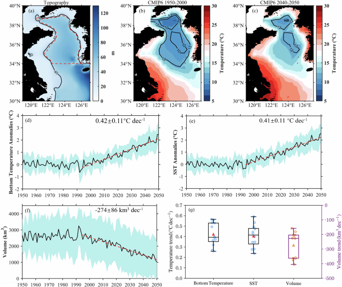
a The topography in the YS with the black contour indicating the 40 m depth and the red dashed line marked the YSCWM generation region. The distribution of the multi-model mean bottom temperature in August averaged over b 1950–2000, and c 2040–2050. The temporal variation of the multi-model mean d T_CWM in August, e the SST_CWM in March, and f the YSCWM volume for 1950–2050. Shadings indicate the standard deviations between models and the dashed lines show the linear trends of each time series during 2001-2050 with its magnitude shown in texts. g Boxplots as in Fig. 1b, but for August T_CWM, March SST_CWM, and YSCWM volume.

Full size image

To quantify the intensity change of the YSCWM, we define the YSCWM generation region as the area north of 34°N within 40 m isobath, which coincidences with the 12 °C isotherm during 1950-2000 (Fig. 2a, b). The YSCWM intensity is then evaluated by the bottom temperature, defined as the temperature at the deepest ocean level in numerical models, averaged over this region (T_CWM) in August, with warmer the temperature weaker the YSCWM intensity. As depicted in Fig. 2d and g, T_CWM in August shows a linear increasing trend of 0.42 ± 0.11 °C dec⁻¹ after 2000, 16% weaker than the annual SST trend in the entire YS (0.50 ± 0.13 °C dec⁻¹).

Relation Between the Winter SST and YSCWM Intensity

As the YSCWM originates from the vertically homogeneous cold water in winter^12,13, we compare the increasing rate of the winter SST over the YSCWM generation region (SST_CWM) with that of T_CWM in August. It is shown that the temporal variation of T_CWM in August correlates well with that of SST_CWM in March (Fig. 2d, e), both show an increasing trend post-2000 with a correlation coefficient of 0.98. The warming rate of March SST_CWM is 0.41 ± 0.11 °C dec⁻¹ (Fig. 2e, g), nearly the same as that of T_CWM in August (0.42 ± 0.11 °C dec⁻¹). The consistency between the trend of T_CWM in August and SST_CWM in March holds in all 12 models (Fig. 3a) with the correlation coefficient between August T_CWM trends and March SST_CWM trend of 0.93.

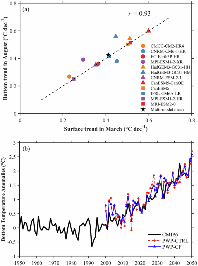
a Scatter plot between August T_CWM and March SST_CWM for 12 CMIP6 models. The linear fit (black line) is shown with the correlation coefficient in text. b the temporal variation of August T_CWM during 2001–2050 derived from the PWP-CTRL (red) and PWP-CF (blue) superposed on that from CMIP6 multi-model mean series (black).

Full size image

To further resolve the dynamical connection between the SST_CWM in winter and T_CWM in summer, we conducted two sensitivity experiments based on the one-dimensional Price–Weller–Pinkel (PWP) mixed layer model³¹. The models are performed for each location of the YSCWM generation region with the monthly mean temperature and salinity profile in March used as the initial condition. The control (CTRL) PWP models are forced by daily net surface heat flux and wind stress until August every year for each climate simulations. As shown in Fig. 3b, the temporal variation of the multi-model mean T_CWM in August after 2001 is well reproduced by the CTRL PWP models with a warming rate of 0.40 °C dec⁻¹ and a correlation coefficient of r = 0.90 between the results of CTRL PWP models and those of CMIP6 models. By substituting the actual sea surface forcings with the respective climatological values between 1950–2000 in all CMIP6 experiments, climatological-forced (CF) PWP models are also performed. The reproduced time series of T_CWM in August also shows an increasing trend of 0.42 °C dec⁻¹ and correlates well with that of the CMIP6 results (Fig. 3b). These results derived from PWP models indicate that the increasing trend of T_CWM in August is primarily determined by the trend of SST_CWM in March, with the long-term changes in sea surface forcing during spring and summer playing a negligible role.

Mechanism driving the YSCWM future changes

To uncover the dynamics responsible for the increase of the winter SST_CWM and summer T_CWM, we perform a temperature budget analysis using the six HighResMIP simulations. Since the vertical distribution of the temperature is nearly uniform in winter (Supplementary Fig. 2), the budget for temperature averaged over the full water column at the YSCWM generation region is calculated. The budget from March 1950 to March 2000 is treated as a baseline and the anomalous budget induced by climate change is obtained by subtracting this baseline from that during March 2001 to March 2050. In the baseline period (Fig. 4a), heat is supplied to the YSCWM generation region by the horizontal advection of warm water (Q_adv) with a warming tendency of 5.3 ± 2.3 °C yr^–1. The warming effect is largely balanced by the surface heat loss to the atmosphere (Q_shf, −4.8 ± 1.5 °C yr^–1) with the horizontal mixing making a minor contribution (Q_mix, −0.5 ± 1.6 °C yr^–1). This balance results in an insignificant tendency of temperature (TD, −0.001 ± 0.014 °C yr^–1) about three orders of magnitude smaller than each heating or cooling term.

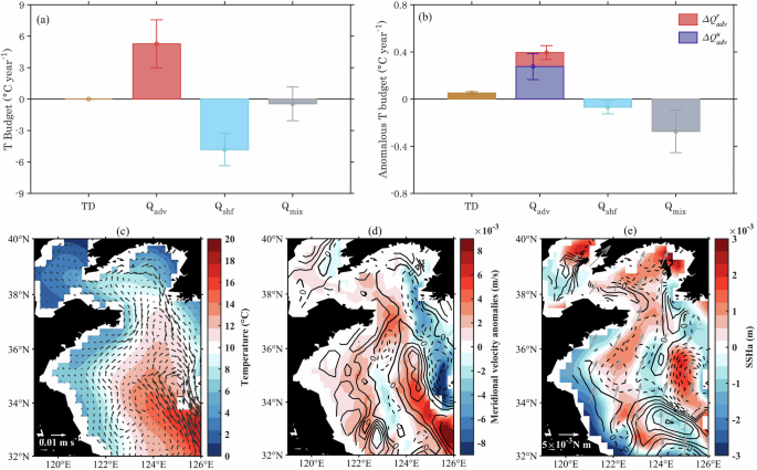
a The baseline temperature budget during 1950-2000. b same as a but for the anomalous temperature budget (2001-2050 relative to 1950-2000). The error bars indicate the standard deviation between models. The horizontal distribution of c the anomalous depth-averaged circulations (arrows) and the mean SST in winter (shading), d the anomalous meridional velocity (shading) and (partial {rm{SSH}}/partial x) in winter, e the anomalous wind stress convergence/divergence (contours, solid line for divergence and dashed line for convergence), anomalous wind stress (arrows) and anomalous SSH (shading) with the horizontal averaged SSH is subtracted.

Full size image

During 2001-2050, the ocean warming with the TD anomaly of 0.05 ± 0.01 °C yr^–1 is caused by the strengthened heat advection (Fig. 4b). The magnitude of Q_adv is strengthened with 0.39 ± 0.17 °C yr^–1 anomalous warming in 2001-2050 relative to that in 1950-2000. This warming effect is largely offset by the change in the horizontal mixing (-0.27 ± 0.18 °C yr^–1). The cooling effect of Q_shf is also strengthened (-0.07 ± 0.06 °C yr^–1) partly compensating for the warming effect. The strengthened heat loss from Q_shf is contributed by the latent heat loss enhancement induced by increased air-sea humidity difference under climate change (Supplementary Fig. 3). The above results are qualitatively consistent in each of the six HighResMIP models, supporting the robustness of the temperature budget analysis (Supplementary Figs. 4 and 5).

To further evaluate the cause of the strengthened heat advection, the anomalous Q_adv ((Delta {Q}_{{rm{adv}}})) is decomposed into the part contributed by the change in ocean current ((Delta {Q}_{{rm{adv}}}^{u})) and the residual ((Delta {Q}_{{rm{adv}}}^{r})) with the detailed decomposition in the method. As shown in Fig. 4b, (Delta {Q}_{{rm{adv}}}^{u}) contributes to 70% of (Delta {Q}_{{rm{adv}}}). This suggests that the response of currents to climate change is the major cause of the winter SST_CWM warming, enhancing the heat transport into the YSCWM generation region.

The change of current field lends further support to the above results. As shown in Fig. 4c, the anomalous currents averaged over the whole water column in winter (December, January, and February, DJF) exhibit northward flows around 34°N, the southern boundary of the YSCWM generation region, indicating the strengthened Yellow Sea Warm Current (YSWC)³². Coinciding with the warm water in the YS trough, the strengthened YSWC injects more heat into the YSCWM generation region, leading to the SST warming in March.

This intensification of the YSWC can be attributed to the anomalous northward wind stress, corresponding to decreased winter monsoon (Fig. 4e). The decreased winter monsoon is caused by reduced land-sea thermal contrast (LSTC) under global warming^33,34. The correlation coefficient between the anomalous LSTC and the anomalous northward wind stress among six HighResMIP simulations is 0.90 (Fig. 5). The change of wind stress causes an anomalous convergence/divergence field, which is negatively correlated with the anomalous sea surface height (SSH) with a spatial correlation coefficient of -0.60 (Fig. 4e). This negative correlation is due to the convergence/divergence of the Ekman transport driven by the wind stress convergence/divergence in the shallow sea³⁵. Consequently, the horizontal gradient of the anomalous SSH field resulting in the intensification of the YSWC under the geostrophic balance, showing a correlation coefficient of 0.66 between the anomalous (partial {rm{SSH}}/partial x) and the anomalous meridional velocity (Fig. 4d).

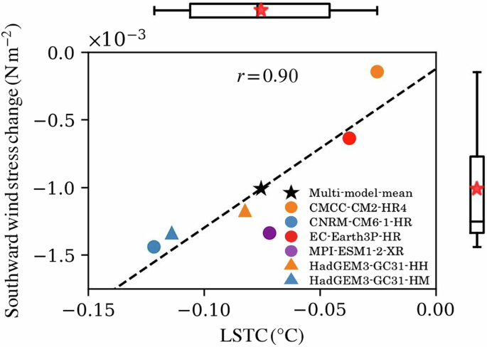
Scatterplot between the change of the LSTC and the North wind intensity in winter (December, January, and February) during 2001–2050 relative to that during 1950–2000. The least-squares linear fit (black line) is shown with the correlation coefficient in text. The boxplot for the change of LSTC (top) and North wind intensity (right) is also shown.

Full size image

In this study, we show the intensity and volume change of a unique BCWM, the Yellow Sea cold water mass (YSCWM), in response to climate change. Based on climate model projections under the high emission scenario (SSP5-8.5) in CMIP6, we find that the volume of the YSCWM with temperature less than 12 °C in August is projected to decrease by 48% by 2040–2050. Meanwhile, the bottom temperature in the YSCWM generation region in August exhibits a linear increasing trend of 0.4 ± 0.1 °C dec⁻¹ corresponding to a decline in the YSCWM intensity. The warming of bottom temperature is closely connected to the SST increase during the previous winter, with minimal influence from long-term change of the surface forcing during spring and summer. Through temperature budget analysis, we attribute the winter SST increase to the strengthened Yellow Sea Warm Current (YSWC) and the associated enhancement of warm water transport, which is driven by a weakened winter monsoon.

Nowadays, offshore aquaculture is developed under the pressure of nearshore fishery¹⁷. Notably, in 2018, an offshore platform-based fish farming facility “Deep Blue 1” was launched in the YSCWM for culturing salmon and trout^36,37. Given the limited mobility of offshore aquaculture, timely prediction of hydrological changes is essential for adapting to the change. For example, the aquaculture cages in Deep Blue 1 will sink below 40 m depth during summer and autumn³⁸, to avoid warm water exceeding 18 °C ensuring the growth of salmon and trout³⁶. However, it remains uncertain whether the temperature around this depth will remain below 18 °C threshold under climate change. To investigate the potential impact of climate change on offshore aquaculture, we estimate the projected changes in temperature at 40–50 m (T_40-50) in October, as it represents the warmest period with the intensified vertical mixing in autumn transports surface warmer water to this level^39,40. As shown in Fig. 6a, the projected multi-model mean T_40-50 in October will exceed 18 °C from 2040 onwards. During 2040–-2050, the “safe area” (T_40-50 < 18 °C) will shrink substantially by 39.3% to the north relative to that during 1950-2000 (Fig. 6b and c).

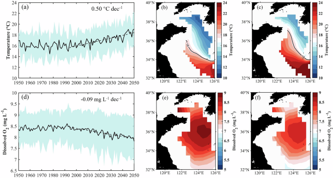
a The multi-model mean temporal variation of temperature averaged over the YS north of 34°N between 40–50 m in October with the shading indicating one standard deviation of the twelve CMIP6 models. The dashed line shows the linear trend from 2001-2050 with its magnitude in legend. The distribution of temperature between 40–50 m depth in October over b 1950–2000, and c 2040–2050 with the 18 °C isotherm denoted by black line. d–f same as a–c but for the dissolved oxygen in the six ESM-BGC models.

Full size image

The biogeochemical properties will change in response to the warming and circulation changes⁶. Ocean deoxygenation is one of the most serious threats to marine life under climate change^41,42,43. In response to the warming and circulation changes⁶, the dissolved oxygen in six ESM-BGC models are also projected to decrease substantially, threatening the survival of plankton and fish in the YSCWM. In October, the dissolved oxygen concentration at 40–50 m depth shows a declining trend of 0.09 ± 0.04 mg (L dec)⁻¹ during 2000-2050, resulting in a 5.3% decrease by 2050 (Fig. 6d–f). This decline is over two times greater than the global estimates for the past 50 years (∼2% globally)^44,45,46. The decrease in saturation concentration⁴⁷ is the primary cause of the reduction of dissolved oxygen concentration due to the oxygen solubility decrease induced by temperature increase in ESM-BGCs (Supplementary Fig. 6). The strengthening YSWC is another potential factor for the reduction of the dissolved oxygen over the YS as it can transport more low-oxygen water from the open ocean into the YS. However, this dynamic is weak in the ESM-BGCs due to the underestimation of the strengthened YSWC in low-resolution models. Therefore, the marine anoxic in the YS might be more severe than indicated above. The ocean warming and the reduction in O₂ levels under the high emission scenario could substantially threaten the future survival of plankton and fish in the YSCWM, and further influence the sustainable development of the off-shore marine aquaculture.

Observational and Reanalysis data

To evaluate the performance of the CMIP6 models in the YS, the observational based and reanalysis dataset are used in this study. The monthly SST is obtained from Hadley Centre Sea Ice and Sea Surface Temperature version 2 (HadISST) datasets for 1950–2022⁴⁸, and Optimum Interpolation SST (OISST) datasets for 1981–2022 obtained from NOAA National Centers for Environmental Information. The monthly climatological sea bottom temperature for 1951-2017 is obtained from the World Ocean Atlas 2018 (WOA18)⁴⁹. For reanalysis data, the Global Ocean Physics Reanalysis (GLORYS) product for 1993–2020 is obtained from E.U. Copernicus Marine Service Information.

CMIP6 Simulations

We select 12 CMIP6 coupled global climate models in this study based on their performance in reproducing the YSCWM in summer (Supplementary Table 1 and Fig. 1). Each model contains a historical run starting from 1950 and forced with historical forcings up to 2014, and a future run forced with greenhouse gases under the equivalent SSP5-8.5 scenario during 2015–2050. The name and the nominal resolutions in the atmospheric and oceanic components of these models are listed in Supplementary Table 1.

The Price-Weller-Pinkel (PWP) mixed layer model

The Price-Weller-Pinkel mixed layer model is a one-dimensional “shear instability” model that attempts to simulate the time evolution and near-surface vertical structure of temperature and salinity in response to the air-sea heat and freshwater fluxes³¹. In this study, we use the PWP model to examine the connection between the winter SST and the YSCWM intensity in summer. The PWP model is performed for each location of the YSCWM generation region. The monthly mean temperature and salinity profile in March of each location is used as the initial condition. The model is forced until August every year by daily air-sea heat flux and wind stress obtained from linear interpolation of the monthly mean output in the CMIP6 experiments. The surface freshwater flux is excluded as its impact on the bottom temperature change is negligible.

Temperature budget analysis

To investigate the dynamics of YSCWM warming in response to climate change, a full-column depth-averaged temperature budget derived under the rigid lid approximation is used:

where h is the depth of sea bottom, T is the potential temperature, u = (u, v) is the horizontal velocity, ({nabla }_{h}=(partial /partial x,partial /partial y)), and the angle brackets denote the horizontal average. The term on the left-hand side of Eq. (1) is the tendency of temperature (TD). On the right-hand side, the first term (Q_adv) is contributed by the horizontal advection, and the second term ({Q}_{{rm{shf}}}={F}_{{rm{shf}}}/({rho }_{0}{c}_{p}h)) measures the contribution from the net sea surface heat flux (F_shf, defined positive downward) with ({rho }_{0}) the reference density of the ocean and ({c}_{p}) the ocean specific heat capacity. The last term Q_mix denotes the contribution from the subgrid-scale vertical and horizontal mixing and is calculated as the residue of the temperature budget. All terms in Eq. (1) are computed with the monthly averaged output from CMIP6 models.

The temperature budget averaged from March 1950 to March 2000 is treated as a baseline and the anomalous temperature budget induced by climate change is obtained by subtracting this baseline from that averaged over March 2001 to March 2050. To further evaluate the cause of Q_adv anomaly to the baseline ((Delta {Q}_{{rm{adv}}})), (Delta {Q}_{{rm{adv}}}) is decomposed as:

where the overbar denotes the temporal average over the baseline period, March 1950 to March 2000, (Delta) represents the anomaly of the temporal average over March 2001 to March 2050 relative to the baseline. The first term on the right-hand side of Eq. (2) ((Delta {Q}_{{rm{adv}}}^{u})) is the contribution of (Delta {Q}_{{rm{adv}}}) from the change of current intensity due to climate change. The second and the third terms are parts of (Delta {Q}_{{rm{adv}}}) caused by the increase of temperature and the change of temporal correlation relation between u and T, respectively. These two terms are treated as the residue of (Delta {Q}_{{rm{adv}}}) denoted by (Delta {Q}_{{rm{adv}}}^{r}).

The land-sea thermal contrast

The land-sea thermal contrast (LSTC) is defined as the difference of mean surface air temperature between land and sea within a 2° band around the coast³³:

where ({T}_{{rm{land}}}^{{rm{air}}}) and ({T}_{{rm{sea}}}^{{rm{air}}}) are the surface air temperature averaged over the 2° band on landward side and seaward side from the coast, respectively.