Check-probe spectroscopy of lifetime-limited emitters in bulk-grown silicon carbide

Optically active solid-state defects have enabled pioneering experiments in the field of distributed quantum computation^1,2,3,4 and quantum networks^5,6. Proof-of-principle experiments have demonstrated primitives for quantum error correction^1,2,3 and the realisation of a three-node network^7,8. Key to these applications is the ability to connect multiple emitters via their coherent spin-optical interface, with many applications requiring narrow, stable optical transitions^6,7.

Spectral diffusion of the transitions, caused by fluctuating charge impurities within the bulk material or at the surface, poses a major challenge, especially when emitters are integrated in nanostructures^9,10,11,12. Moreover, laser pulses used to probe or manipulate the emitter can exacerbate such diffusion^10,13. Experimental techniques that enable the quantitative study of spectral diffusion and its timescales provide insight into the environmental charge dynamics, potentially allow for targeted optimisation of material properties and fabrication processes, and enable pathways to mitigate diffusion through pre-selection^13,14. However, commonly used methods may significantly disturb the system through continuous laser illumination, complicating the unambiguous determination of transition line widths and diffusion rates under different laser illumination conditions^{9,10,15,16,17}.

Here, we introduce a comprehensive check-probe spectroscopy toolbox for characterising and mitigating spectral diffusion of single solid-state emitters. Our methods offer high-bandwidth, quantitatively extract diffusion and ionisation rates, and introduce minimal system disturbance from laser illumination, enabling accurate measurements even in heavily diffusive environments. Additionally, our work provides a framework for the quantitative analysis of heralded preparation of the charge environment, which has become an indispensable tool to mitigate spectral diffusion in quantum network and other experiments^{3,7,8,13,14,18}.

We apply these methods to study single k-site V_Si (V2) centres (a next-generation candidate for quantum networks^15,19,20), embedded in nanopillars etched in commercially available bulk-grown 4H-silicon carbide (SiC)^21,22. This system exhibits a high degree of spectral diffusion (>1 GHz diffusion-averaged linewidth), typical for single quantum emitters in bulk-grown silicon or silicon carbide^23,24. First, we determine spectral diffusion rates with and without laser illumination. Using this knowledge, we select configurations of the system with narrow spectral transitions, which can be tuned over the breadth of the inhomogeous linewidth and can be stored for over a second and accessed on-demand. Finally, through the observation of Landau-Zener-Stückelberg interference²⁵, we determine the optical coherence time to be: T₂ = 16.4(4) ns, consistent with the lifetime limit for these defects²⁶.

Although high-purity epitaxial layers provide a starting point with less spectral diffusion^15,19,27 (Supplementary note 8), our observation of lifetime-limited coherence in nanostructures in bulk-grown silicon carbide, hints towards the possibility of using such mass-fabricated material for quantum technology development and applications. Furthermore, the techniques developed here might facilitate the targeted optimisation of material and fabrication recipes, and can be readily transferred to other platforms^{18,24,28,29,30}.

Single V2 centres in bulk-grown silicon carbide

We consider spectral diffusion caused by fluctuating charges in the environment of the emitter, for example, associated with material impurities or surface defects that modify the optical transition frequency via the Stark shift^31,32,33,34. Although these dynamics are largely frozen at cryogenic temperatures¹⁷, charges can still be mobilised through laser illumination used for the optical addressing of the emitter^9,10,17,24 (Fig. 1a). In particular, charges can be excited to the conduction (or valence) band via a single-photon process if the energy difference from the occupied charge state is smaller than the associated energy of the laser frequency (Fig. 1b). Subsequent decay to a different spatial position causes fluctuations in the electric field at the location of the emitter^10,17.

a Schematic of the system. A single V2 centre in SiC is surrounded by charges (yellow circles) associated to intrinsic residual impurities³⁵. Under laser illumination, these charges can be mobilised after excitation to (from) the conduction (valence) band, indicated by blue and red wiggly lines. b Energy diagram, depicting the V2 centre’s optical transitions (left) and possible laser-induced charge dynamics of the (unknown) impurities in the environment (right). The spin-dependent A₁ and A₂ transitions can be excited with a tunable, near-infrared (NIR) laser (916 nm, red arrow), while a high-energy repump laser (785 nm, blue arrow) is used to scramble the charge state of the V2 centre and its environment. The ground-state spin ((S=frac{3}{2})) can be manipulated with microwave (MW) radiation. c Scanning-electron-microscopy image of a sample used in this work, which is diced from a 4 inch commercially available 4H-SiC bulk wafer. Nanopillars (~500 nm diameter) are fabricated to improve the photon collection efficiency. d Representative low-temperature (4K) emission spectrum of a V2 centre under repump-laser excitation, showing the characteristic zero-phonon line at 916 nm (red highlight). e Experimental sequence of the diffusion-averaged photoluminescence-excitation spectroscopy (PLE). The frequency f₁ of the NIR laser (red) is scanned over the V2 zero-phonon line, while emission in the phonon sideband is collected. The repump laser (blue) scrambles the charge state of the emitter and its environment before every repetition (total N). f Measured PLE spectrum. Averaging over many charge-environment configurations results in a single, broad peak (2.4(1) GHz FWHM) that encompasses the A₁ and A₂ transitions (separated by ~1 GHz). The laser frequency is offset from 327.10 THz.

Full size image

Although our methodology applies to a range of emitter types, materials, and operating temperatures, this work specifically considers single k-site V_Si (V2) centres in commercially available bulk-grown silicon carbide at 4K. In this material, diffusion is likely caused by charges associated with residual defects and shallow dopants (concentrations ~10¹⁵ cm⁻³) that are created during the growth process³⁵. We apply two types of lasers: a 785 nm ‘repump’ laser for charge-state reinitialisation (~10 μW), and two frequency-tunable near-infrared (‘NIR’) lasers (~10 nW) for resonant excitation of the V2 centre’s spin-dependent A₁ and A₂ zero-phonon-line transitions (Fig. 1b and d)¹⁹.

We fabricate nanopillars that enhance the optical collection efficiency (Methods), to mitigate the effects of the unfavourable dipole orientation in c-plane 4H-SiC (Fig. 1c). In about one in every 10 pillars, we observe a low-temperature spectrum with a characteristic zero-phonon line at 916 nm (Fig. 1d), hinting at the presence of single V2 centres confined to the nanopillars. The dimensions of the nanopillar, with a diameter of ~500 nm and a height of ~1.2 μm, mean that surface- and fabrication-related effects might contribute to the diffusion dynamics.

Photoluminescence excitation spectroscopy

First, we measure the V2 diffusion-averaged optical absorption linewidth via photoluminescence excitation spectroscopy (PLE). By repeatedly interleaving repump pulses (‘R’, 10 μs, 10 μW) with NIR pulses at a varying frequency f₁ (10 μs, 10 nW, Fig. 1e), we randomise the V2 charge environment before each repetition, effectively averaging over many spectral configurations. In a system without spectral diffusion, we would expect to observe two distinct narrow lines (FHWM of ~26 MHz and ~11 MHz), separated by Δ ≈ 1 GHz^19,26,36, corresponding to the separation of the A₁ and A₂ transitions. However, we observe a broad Gaussian peak (2.4(1) GHz, see Fig. 1f), hinting at a high degree of spectral diffusion, consistent with comparable experiments in similar bulk semiconductor materials^24,28.

In order to probe the individual A₁ and A₂ transitions, we employ a two-laser PLE scan²⁸. Compared to the sequence in Fig. 1e, we now fix frequency f₁ close to the middle of the broad resonance (Fig. 1f) and add a second NIR laser at frequency f₂ (Fig. 2a). We observe a significant increase in the detected count rate when the frequency difference satisfies: f₂ − f₁ ≈ Δ = 954(2) MHz, explained by a strong reduction in optical pumping (which otherwise quickly diminishes the signal²⁸). Importantly, the relatively narrow resonance condition (FWHM of 89(9) MHz) observed in Fig. 2b suggests that the homogeneous linewidth is much narrower than the diffusion-averaged linewidth in Fig. 1f.

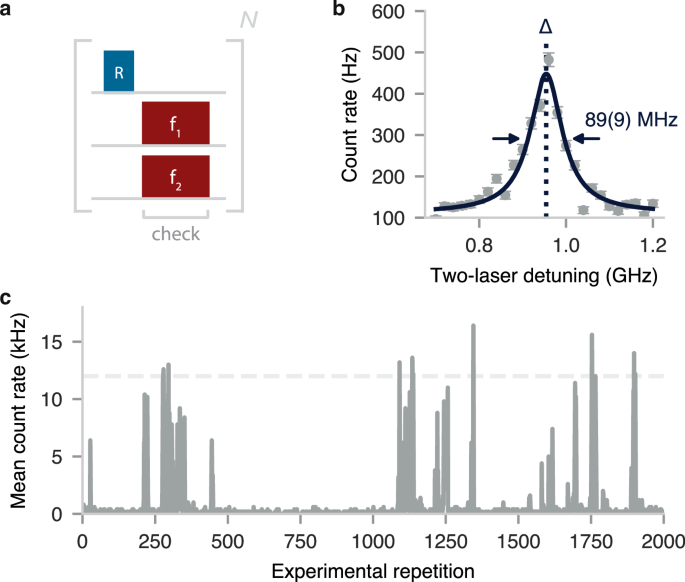
a Experimental sequence. A short (10 μs, 10 μW) high-energy (785 nm) repump laser pulse (‘R’) partially scrambles the charge state of both the environment and the V2 centre. Emission is collected during the ‘check’ block, when two NIR lasers at frequencies f₁ and f₂ are turned on (approximately resonant with the broad peak in Fig. 1g). b We observe an increase in count rate if the laser frequency difference is equal to Δ = 954(2) MHz, the spacing between the A₁ and A₂ transitions. A Lorentzian fit obtains an FWHM of 89(9) MHz. c Detected mean count rate per experimental repetition, when the length of the ‘check’ block is set to 5 ms. In most repetitions, the defect is off-resonant with the lasers. When the A₁ and A₂ transitions coincide with laser frequencies f₁ and f₂, we observe significant emission (≫1 kHz). Thresholding (dashed line) on the detected counts can be employed to prepare specific (i.e. ‘on resonance’) spectral configurations of the V2 centre.

Full size image

Next, we fix the laser frequency difference to Δ and record the counts per experimental repetition (Fig. 2c). We obtain a telegraph-like signal, consistent with a single V2 centre that is spectrally diffusing. Such a signal allows for the implementation of a charge-resonance check^14,18, which probes whether the V2 centre is in the desired negative charge state, and its two transitions are resonant with the NIR lasers. If the number of detected counts passes a threshold T (e.g. the grey dashed line in Fig. 2c), we conclude that the defect was on resonance in that specific experimental repetition, allowing for post-selection (or pre-selection) of the data. In the following, we will explore how such post-selection tactics can be exploited to gain insights in the spectral diffusion dynamics.

Check-probe spectroscopy: ionisation and diffusion dynamics

Next, we develop a method to measure the ionisation and spectral diffusion dynamics of the V2 centre. Currently, various experimental techniques exist, based either on tracking the transition frequency with subsequent PLE scans^10,15,16, or on autocorrelation-type measurements^9,37. The former method struggles with measuring dynamics faster than the acquisition timescale of a single scan^15,38 (yielding ~Hz bandwidth typically, see also Supplementary Fig. 8). The latter, although fast (up to ~GHz bandwidth), offers limited flexibility for probing diffusion under external perturbations⁹.

Here, we take a different approach, based on a pulsed check-probe scheme as outlined in Fig. 3a. Following a charge-randomization (repump) step, two ‘check’ blocks are executed (as in Fig. 2a), separated by a perturbation of the system (grey block marked ‘X’). Such a perturbation might consist of turning on (or off) specific lasers (e.g. NIR or repump) during the delay time t. This pulsed scheme allows for the isolation of diffusion originating from the perturbation from other sources with a high bandwidth. The timescales for the perturbation are only limited by the modulation speed and timing resolution of the laser pulses and perturbation, providing potential bandwidths in the gigahertz regime (e.g. using electro-optic modulation).

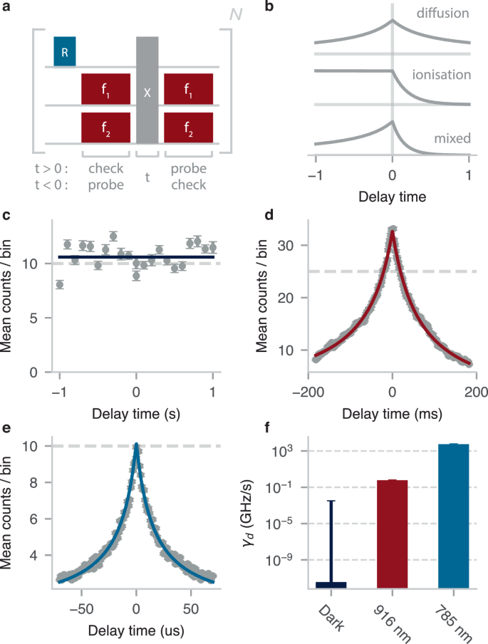
a Experimental sequence. A ‘check’ block (2 ms, 20 nW) is followed by a system perturbation (marked ‘X’), which here consists either of turning off the lasers (c), turning on the NIR lasers (d), or turning on the repump laser (e). A second block (2 ms, 20 nW) probes whether the defect has diffused away, or has ionised (denoted ‘probe’). Data is post-selected by imposing a minimum-counts threshold (T), heralding the emitter on resonance in the first (second) block and computing the mean number of counts in the second (first) block, which encodes the emitter brightness at future (past) delay times t. b Schematic illustrating the expected signal (according to Eq. (1)), when either ionisation or spectral diffusion is dominant (setting γ_r ≈ 0). c No significant spectral diffusion or ionisation is observed when the lasers are turned off. The solid line is a fit to the data using Eq. (1). Dashed grey line denotes the set threshold (in a 2 ms window). d Experiment and fit under 20 nW of NIR laser power (916 nm). e Experiment and fit under 1 μW of repump laser power. f Extracted saturation-diffusion rates, obtained at laser powers of ~20 nW (resonant) and ~5 μW (repump). See supplementary Fig. 3 for underlying data and error analysis.

Full size image

Importantly, one can either post-select on high counts (i.e. ‘check’) in the block before, or after the perturbation, effectively initialising the emitter on resonance at the start, or at the end of the experiment. By ‘probing’ the emitter brightness after (before) the perturbation, we effectively track its evolution forward (backward) in time, denoted as delay time t > 0 (t < 0) in Fig. 3a. This allows for the distinction between time-symmetric and non-time-symmetric perturbation processes (e.g. spectral diffusion or ionisation of the emitter, see Fig. 3b), as opposed to evaluating the purely symmetric autocorrelation function⁹.

To quantitatively describe the signal, we derive an analytical expression that takes into account spectral diffusion and ionisation of the emitter. In this system, spectral diffusion is mainly caused by laser-induced reorientation of charges surrounding the defect, whose dynamics can be approximated by a bath of fluctuating electric dipoles¹⁷. To model this, we employ the spectral propagator formalism^38,39, which describes the evolution of the spectral probability density function in time, and whose form is given by a Lorentzian with linearly increasing linewidth γ(t) = γ_d ∣t∣³⁹ (with γ_d the effective diffusion rate). Note that this description is valid only at short timescales (γ_d ∣t∣ ≪ 1 GHz), as the spectral probability density should eventually converge to the diffusion-averaged distribution observed in Fig. 1f³⁹. Furthermore, we take the spectral propagator to be time-symmetric, and model the ionisation (charge recapture) of the emitter as an exponential decay of fluorescence, governed by rate γ_i (γ_r).

The mean number of observed counts at delay time t can be described by (Supplementary note 1):

with C₀ the mean number of observed counts at t = 0, Γ the emitter’s (Lorentzian) homogeneous linewidth, and γ_d, γ_i, γ_r > 0. Note that Eq. (1) in general does not obey time-inversion symmetry (for γ_i ≠ γ_r), and in specific cases allows for a clear distinction between ionisation and diffusion processes (e.g. if γ_r ≈ 0, see Fig. 3b). Next to that, the functional form of Eq. (1) captures information about the type of processes at play: emitter charge dynamics are described by an exponential decay while spectral diffusion has a power law dependence.

We experimentally implement the sequence for three distinct perturbations: (i) no laser illumination (Fig. 3c), (ii) illumination with the two NIR lasers (20 nW, Fig. 3d), and (iii) illumination with the repump laser (1 μW, Fig. 3e). We observe a wide range of dynamics, from the microsecond to second timescale, and observe excellent agreement between the data and the model (solid lines are fits to Eq. (1)).

To quantitatively extract ionisation and diffusion rates under the perturbations, we set Γ = 36 MHz, (independently determined in Fig. 4e). We find that extracted rates are weakly dependent on the set threshold value, resulting from non-perfect initialisation on-resonance, but converge for higher T (Supplementary note 2). Averaging over a range of threshold values, we find diffusion rates γ_d = 0.00(2) GHz s⁻¹, 0.60(2) GHz s⁻¹, 2.4(2) × 10³ GHz s⁻¹, for perturbations (i), (ii) and (iii), respectively. Note that for larger Γ (e.g. at elevated temperatures³⁶), the relative contribution of slow spectral diffusion decreases and the measurement uncertainty for γ_d increases. In the dark, where almost no diffusion is apparent, the fit only converges if we set γ_i, γ_r = 0, which is a reasonable assumption at 4 K, given the deep-level nature of the V2 centre^17,35.

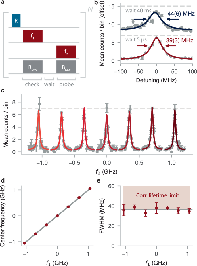
a Experimental sequence. A resonant laser at f₁ and a microwave (MW) pulse resonant with the ground-state spin transition act as a resonance check, initialising the optical transition near f₁. Next, a second laser probes the defect emission at f₂ (for 2 ms), yielding a measurement of the linewidth with minimal disturbance. b Experimental data showing narrow optical transitions, with the bottom (top) data corresponding to a waiting time of 5 μs (40 ms) between the f₁ and f₂ laser pulses (offset for clarity). Data are fitted to a Lorentzian with a FWHM of 39(3) MHz (44(6) MHz). The counts threshold is set to T = 7 during the f₁ pulse. c Data and fits as in (b)(bottom), scanning f₂ around f₁, when f₁ is set at different frequencies (various shades of red) within the broad diffusion-averaged line measured in Fig. 1g. d Measured resonance center frequency as a function of the set f₁ frequency (solid grey line: f = f₁). The defect emission frequency can effectively be tuned over a GHz range. e Corresponding linewidths extracted from (c), with inverse-variance weighted mean 36(1) MHz (solid grey line). The shaded region denotes the expected minimum linewidth (~36 MHz), given the lifetime limit of ~20 MHz, and correcting for power broadening (~26 MHz, Fig. 5j) and residual inhomogeneous broadening (~15 MHz, Eq. (2)).

Full size image

Ionisation effects are only observed under the NIR-laser perturbation, due to the short diffusion timescale during the repump-laser perturbation (resulting in divergent fit results for γ_i and γ_r). From the data in Fig. 3d, we extract γ_i = 1.0(2) Hz and γ_r = 0.03(4) Hz. Correcting for reduced ionisation when the V2 centre is off-resonance with the NIR lasers results in an ionisation rate ({gamma }_{{rm{i}}}^{0}=3(1),,text{Hz},) (see Supplementary note 1).

We repeat the experiments for various laser powers, and observe a saturation-type behaviour of the diffusion rates, both under NIR-lasers and repump laser excitation (Supplementary Fig. 3). The higher saturation-diffusion rate measured for the repump laser is likely due to the larger fraction of charge traps that can be ionised via a single-photon process (see Figs. 1b and 3f). Different V2 centres in the material, show some variation in the (saturation) diffusion rates (Supplementary Figs. 4 and 8). Note that the behaviour at powers beyond those accessed in these experiments will determine if spectral stability persists under repeated fast optical π-pulses, as commonly used for remote entanglement generation experiments^7,14,18.

Check-probe spectroscopy: linewidth

Having established the spectral diffusion timescales, we characterise the homogeneous linewidth. We use an optical spectroscopy method that leverages the high-bandwidth nature of the check-probe scheme (similar to ref. ⁴⁰) to mitigate linewidth broadening due to spectral diffusion. This is in contrast with conventional ‘scanning PLE’, which averages over diffusion dynamics faster than the acquisition timescale needed to obtain sufficient data over the full scanning frequency range^{10,13,15,16,19,41} (typically ~s timescale, Supplementary Fig. 8. This is especially relevant for systems that are sensitive to laser-induced diffusion (such as the one considered here) for which the check-probe scheme only requires laser illumination on timescales short compared to the laser-induced diffusion timescales.

First, we execute an alternative implementation of the ‘check’ block (compared to Figs. 2a and 3a), that consists of a single NIR-laser pulse at f₁, together with an MW pulse that mixes the spin states (Fig. 4a). By post-selecting on high counts, either the A₁ or A₂ transition is initialised on-resonance with f₁. A second laser is used to probe the defect emission at a frequency f₂ immediately thereafter (~μs timescale, here limited by the microprocessor clock cycle). By studying the mean number of counts during the f₂ pulse, (an upper bound for) the homogeneous linewidth can be extracted (Fig. 4b).

We introduce a quantitative model for the signal that extracts the homogeneous linewidth and considers the residual inhomogeneous broadening resulting from non-perfect initialisation on-resonance. To this end, we compute the spectral probability density immediately after the ‘check’ block, as a function of the number of detected photons m ≥ T using Bayesian inference (see Supplementary note 4):

with f the emitter frequency, λ(f) the pure (i.e. homogeneous) spectral response of the emitter, Γ_i[a, z] the incomplete Gamma function and N_T a normalisation constant (Supplementary note 4). The expression in Eq. (2) is strongly dependent on T, with higher threshold values leading to distributions that are sharply peaked around f₁. Note that this analysis assumes negligible laser-induced diffusion during the ‘check’ block, placing limits on the used laser power and the block’s duration (≪1/γ_d).

The measured signal, i.e. the mean number of detected counts in the ‘probe’ block is then given by:

where * denotes the linear convolution. Importantly, as both terms in Eq. (3) contain λ(f), the pure spectral response can be recovered by varying T in post-processing (Supplementary note 4). In particular, for the Lorentzian spectral response:

with FWHM Γ and on-resonance brightness C₀, the signal converges to: C(f) → λ_L(f − f₁) at high threshold values (({T},gg ,max left[lambda (f)right])), simplifying the analysis (Supplementary note 4).

We demonstrate the check-probe spectroscopy method on the same V2 centre as used in Figs. 1f, 2 and 3 (Methods), and observe narrow Lorentzian resonances around the f₁ laser frequency (39(3) MHz at T = 7, see Fig. 4b). Correcting for residual broadening by fitting Eq. (3) to the data for 1 ≤ T ≤ 13 (using Eqs. (2) and (4)), we extract: C₀ = 6.5(1) counts (3.22(7) kHz count rate) and Γ = 33(1) MHz. This spectrum (as well as the those measured in Fig. 5) corresponds to an average over the A₁ and A₂ transitions, resulting in: (Gamma approx ({Gamma }_{{{rm{A}}}_{{rm{1}}}}+{Gamma }_{{{rm{A}}}_{{rm{2}}}})/2) (<5% deviation, assuming equal initialisation probability, see Supplementary note 5). Note that this ambiguity between the transitions can be fully resolved by executing the ‘check’ block with two NIR lasers, as in Fig. 2. The discrepancy between the extracted mean linewidth and the mean lifetime limit (~20 MHz) is well-explained by power-broadening, with optical Rabi frequencies estimated to be ~26 MHz (next section, see Fig. 5j).

Next, to verify our previous inference that spectral diffusion is virtually absent without laser illumination (Fig. 3c), we insert a 40 ms waiting time between the f₁ and f₂ pulses (Fig. 4b, top), which does not increase the linewidth within the fit error (T = 7). Importantly, this allows for the preparation of the transition at a specific frequency, ‘storing’ it in the dark, so that the V2 centre can be used to produce coherent photons at a later time. Furthermore, the broad nature of the diffusion-averaged linewidth depicted in Fig. 1f, enables probabilistic tuning of the emission frequency over more than a gigahertz¹⁸. We demonstrate this by varying the f₁ frequency, initialising the emitter at different spectral locations, and probing the transition with the NIR laser at frequency f₂ (Fig. 4c–e). Such tuning of the V2 emission frequency without the need for externally applied electric fields^31,32 might open up new opportunities for optically interfacing multiple centres.

Landau-Zener-Stückelberg interference

To further benchmark the check-probe spectroscopy method, we use it to resolve Landau-Zener-Stückelberg (LZS) interference fringes in the optical spectrum²⁵. Such fringes demonstrate coherent control of the orbital states of the V2 defect using MW frequency electric fields, and enable the independent determination of the optical coherence and Rabi frequency²⁵, allowing for the separation of their contributions to the linewidths measured in Fig. 4.

LZS interference fringes can arise when a strong AC electric field shifts the optical transition across the laser frequency multiple times within the coherence time of the emitter^32,42. Each time a crossing occurs, the emitter is excited with a small probability amplitude and associated ‘Stückelberg’ phase. These amplitudes can interfere constructively or destructively, creating fringes in the spectrum (see ref. ²⁵ for an extensive review on the phenomenon).

In our setup, MW radiation is applied by running an AC current through an aluminium alloy wire spanned across the sample (Fig. 5a). The original purpose of the wire is to enable mixing of the ground-state spin in the ‘check’ and ‘probe’ blocks used in Fig. 4. However, this geometry also creates significant electric fields at microwave frequencies (Fig. 5a). Taking the defect ground and excited states as basis states ((leftvert grightrangle =leftvert 0rightrangle) and (leftvert erightrangle =leftvert 1rightrangle)), the (optical) evolution of the system is described by the Hamiltonian (in the rotating frame of the emitter)⁴²:

where Ω is the optical Rabi frequency, δ is the detuning between the optical transition and the laser frequency, A is the stark-shift amplitude (which scales with the electric field amplitude), ω is the MW driving frequency and σ_x, σ_z are the Pauli spin matrices. For the experimental parameters used here, the system is considered to be in the ‘fast-passage’ regime (defined as A ω ≫ Ω²²⁵), meaning the excitation probability amplitude during a single crossing is small (Methods). In this regime, the spectral response of the emitter can be described by²⁵:

where C₀ is the on-resonance emitter brightness for A = 0, ({Omega }_{k}=Omega ,{J}_{k}left(frac{A}{omega }right)), with J_k the Bessel function, and T₁, T₂ are the emitter’s optical relaxation and (pure-dephasing) coherence times respectively. Figure 5c shows the optical spectrum as a function of A, obtained by evaluating Eq. (6) for our sample parameters. At higher electric field amplitudes (i.e. higher A), multiple characteristic interference fringes appear, spaced by the driving frequency ω (here 70 MHz), creating a complex optical spectrum.

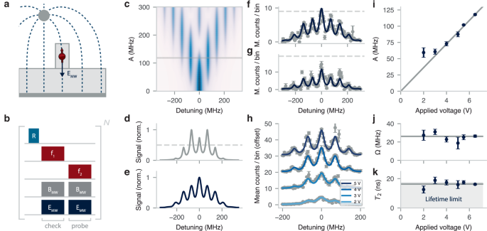
a Schematic showing the electric-field generated by the MW drive, connecting the bond wire and ground plane (dark grey, not drawn to scale), which can generate significant stark shifts. b Sequence, as in Fig. 4a, but now explicitly including the electric field (E_MW). c Characteristic LZS interference pattern (theory) as function of the laser detuning, and the electric field strength A. At higher electric fields, side bands emerge at multiples of the driving frequency ω = 70 MHz. d Line cut through (c) for A = 118 MHz. The dashed line denotes an example threshold T. e The experimental spectrum expected from the situation in (d). The signal differs from the original spectrum as it is weighted over the probability to pass the threshold for different detuning. f Mean detected counts as a function of the two-laser detuning when the MW amplitude is set to 6.5 V, approximately equal to the value in (d). The threshold (T = 10) is set to about half the maximum amplitude, as in (d). The fit function (solid line) is obtained by fitting the dataset for a range of threshold values (see Supplementary Fig. 6). g Same dataset as in (f), but with T = 20. The signal distortion due to the threshold is well-captured by the fit. h Experimental data (grey) and fit (solid lines) as in (f), varying the applied voltage (T = {6, 10, 13, 15}). Data are offset by 10 counts for clarity. i Extracted electric field strength A as a function of the applied voltage. The solid grey line is a linear guide to the eye. j Extracted optical Rabi frequency Ω. Solid grey line denotes the inverse-variance weighted mean. k Extracted optical coherence time T₂. The shaded region denotes the mean lifetime limit: T₂ = 2T₁ ≈ 17 ns. Solid grey line denotes the inverse-variance weighted mean of the data points.

Full size image

Measuring such complex spectra with the check-probe optical spectroscopy method requires taking into account signal distortions arising from the form of the spectral probability density after the check block (Eq. (2)). To see why this is the case, we consider an exemplary theoretical spectrum plotted in Fig. 5d (for A = 118 MHz), where the threshold T is set to about half the maximum signal amplitude (dashed line in Fig. 5d). Such a threshold is passed (with high probability) not only when the central peak is on resonance with f₁, but also when one of the nearest fringes is on resonance with the laser. Computing the resulting weighted signal (inserting Eq. (6) in Eq. (3)) yields the distorted, experimentally expected spectrum shown in Fig. 5e.

To experimentally measure the LZS interference signal, we execute the sequence in Fig. 5b, now explicitly including the electric field components generated by the MW drive. These components were also implicitly present in previously discussed experiments (Fig. 4), but their effects could largely be neglected under the conditions: ω > A and (omega ,>, Gamma approx sqrt{{(pi {T}_{2})}^{-2}+{Omega }^{2}})²⁵. We set the MW driving frequency ω to the ground-state zero field splitting (70 MHz), so that the magnetic field components efficiently mix the spin states^19,43, and set the (peak-to-peak) MW amplitude between the wire and the ground plane to 6.5 V. Figure 5f and g show the measured spectrum for a threshold of T = 10 and T = 20 respectively. The former corresponds roughly to the example threshold in Fig. 5d, and the observed signal matches well with the expected spectrum in Fig. 5e. Setting T = 20 alters the measured spectrum, highlighting the interplay between the threshold and corresponding distortion. The solid lines are generated by a single fit of the complete dataset using Eq. (3) for 1 < T < 21 (post-processed, see Supplementary Fig. 6).

We repeat this procedure while varying the MW amplitude (Fig. 5h) and extract A, Ω and the estimated pure-dephasing T₂ coherence time (Fig. 5i, j and k), keeping ω and the optical relaxation time T₁ = 8.7 ns fixed (again using the mean of the A₁ and A₂ transitions²⁶). For amplitude values above 2 V we observe a linear relation between the MW amplitude and A, as expected. For lower values, a significant deviation is observed, possibly because the system is no longer well-described by the fast-passage limit (i.e. A ω ~ Ω²). Indeed, the optical Rabi frequency is estimated to be 26(1) MHz (weighted mean of Fig. 5j), on the order of (sqrt{A,omega }). Finally, we find a mean T₂ = 16.4(4) ns, approximately equal to the mean lifetime limit (2 T₁ ≈ 17 ns²⁶).

In this work, we introduced a high-bandwidth check-probe scheme that allows for quantitative characterisation of spectral diffusion and ionisation processes under the influence of external perturbations. Our methods enable measurements of the homogeneous transition linewidth of single quantum emitters, under minimal system disturbance.

We applied these methods to study the optical coherence of the V2 centre in commercially available bulk-grown silicon carbide. Despite high levels of spectral diffusion under laser illumination, we reveal near-lifetime-limited linewidths with slow dynamics, enabling the preparation of a frequency-tunable coherent optical transition^18,31,32. Although higher purity materials are likely desired, such coherent optical transitions in bulk-grown SiC might enable nanophotonic device development, testing and characterisation (e.g. cavity coupling, Purcell enhancement) using widely available materials⁴⁴. Studying defects integrated in nanocavities is of special interest, as their proximity to surfaces can significantly alter spectral diffusion dynamics. Future avenues for research in bulk-grown material include investigating the spin coherence properties and the spectral stability under higher-power laser pulses used for long-distance entanglement generation^7,8.

Finally, the presented methods are applicable to other platforms where spectral diffusion forms a natural challenge, such as rare-earth-doped crystals⁴⁵, localised excitons³⁰ or semiconductor quantum dots²⁹, and might enable new insights in the charge environment dynamics of such systems.

Sample parameters

The sample was diced directly from a 4-inch High-Purity Semi-Insulating (HPSI) wafer obtained from the company Wolfspeed, model type W4TRF0R-0200. We note that the HPSI terminology originates from the silicon carbide electronics industry. In the quantum technology context considered here, this material has a significant amount of residual impurities (order ~10¹⁵ cm⁻³ according to Son et al.³⁵) and is hence considered low purity with respect to a concentration of ~10¹³ cm⁻³ typical for epitaxially grown layers on the c-axis of silicon carbide^15,46. On a different sample, diced from a wafer with the same model type, a Secondary-Ion Mass Spectroscopy (SIMS) measurement determined the concentration of nitrogen donors as [N] = 1.1 × 10¹⁵ cm⁻³. In addition to intrinsic silicon vacancies, we generate additional silicon vacancies through a 2 MeV electron irradiation with a fluence of 5 × 10¹³ cm⁻². The sample was annealed at 600 ^∘C for 30 min in an Argon atmosphere. To enhance the optical collection efficiency and mitigate the unfavourable V2 dipole orientation for confocal access along the SiC growth axis (c-axis), we fabricate nanopillars. We deposit 25 nm of Al₂O₃ and 75 nm of nickel on lithographically defined discs. A subsequent SF₆/O₂ ICP-RIE etches the pillars, see figure 1c. The nanopillars have a diameter of 450 nm at the top and 650 nm at the bottom and are 1.2 μm high. We note that, considering the modest efficiency of our detector (≈25% at 950 nm), photon detection rates from the single V2 centres studied here (~15 kHz, see Fig. 2c) – while consistent with other reports on HPSI²² – appear to be high compared to recently reported values on epitaxially grown layers^19,41,43,47. This discrepancy might indicate that the photo-physics, including the meta-stable state dynamics, depend on the material purity, but this has not been further investigated in this work.

Experimental setup

All experiments are performed using a home-built confocal microscopy setup at 4K (Montana Instruments S100). The NIR lasers (Toptica DL Pro and the Spectra-Physics Velocity TLB-6718-P) are frequency-locked to a wavemeter (HF-Angstrom WS/U-10U) and their power is modulated by acousto-optic-modulators (G&H SF05958). A wavelength division multiplexer (OZ Optics) combines the 785 nm repump (Cobolt 06-MLD785) and NIR laser light, after which it is focused onto the sample by a movable, room temperature objective (Olympus MPLFLN 100x), which is kept at vacuum and is thermally isolated by a heat shield. A 90:10 beam splitter that directs the laser light into the objective, allows V2 centre phonon-sideband emission to pass through, to be detected on an avalanche photodiode (COUNT-50N, filtered by a Semrock FF01-937/LP-25 long pass filter at a slight angle). Alternatively, emission can be directed to a spectrometer (Princeton Instruments IsoPlane 81), filtered by a 830 nm long pass filter (Semrock BLP01-830R-25). Microwave pulses are generated by an arbitrary-waveform generator (Zurich Instruments HDAWG8), amplified (Mini-circuits LZY-22+), and delivered with a bond-wire drawn across the sample. The coarse time scheduling (1 μs resolution) of the experiments is managed by a microcontroller (ADwin Pro II). For a schematic of the setup see Supplementary Fig. 9.

Magnetic field

For the check-probe optical spectroscopy measurements in Fig. 4 and Supplementary Fig. 8, we apply an external magnetic field of ≈1 mT along the defect symmetry axis (c-axis). All other experiments are performed at approximately zero field. We apply the field by placing a permanent neodymium magnet outside the cryostat. We align it by performing the sequence depicted in Fig. 1e, with f₁ set at the centre frequency of the broad resonance (Fig. 1f), and monitoring the average photoluminescence (f₁ pulse is set to 2 ms). A (slightly) misaligned field causes spin-mixing between the ({m}_{s}=pm frac{3}{2}) and ({m}_{s}=pm frac{1}{2}) subspace, which increases the detected signal. Minimising for the photoluminescence thus optimises the field alignment along the symmetry axis.

LZS fast-passage regime

The fast-passage regime is defined by: Aω ≫ Ω^2 25, with ω = 70 MHz. From the measurements in Fig. 4, we can estimate: Ω < 40 MHz. Furthermore, we can get a rough estimate for A by approximating the electric field at the defect to be: (Eapprox frac{U}{d}(epsilon +2)/3), with U the applied voltage, d ≈ 500 μm the distance between the wire and the ground plane and ϵ ≈ 10 the dielectric constant of silicon carbide (using the local field approximation³²). There is some debate on the value of the Stark-shift coefficient^31,32. Here, we take the value from ref. ³²: 3.65 GHz m MV⁻¹ and estimate A ≈ 29 MHz for an applied voltage of 1 V. Hence, Aω > Ω² for U > 1 V, and the fast-passage requirement is satisfied for most measurements in Fig. 5. The excellent agreement between the data and our model (especially for higher values of U) and the corresponding extracted values for Ω and A, further justify using the fast-passage solution of the LZS Hamiltonian.

Error analysis

For all quoted experimental values, the value between brackets indicates one standard deviation or the standard error obtained from the fit (unless stated otherwise). The error bars on the mean counts are based on Poissonian shot noise. The uncertainty on fit parameters is rescaled to match the sample variance of the residuals after the fit.