Climate change exacerbates compound flooding from recent tropical cyclones
Introduction
Tropical Cyclones (TCs) are a significant driver of global flood damage1. TC flooding is complex because it involves multiple hydrometeorological and oceanographic drivers that lead to coastal, runoff, and compound flood processes2. TC rainfall and surge—key drivers of compound flooding—are expected to increase in the future3,4,5. However, flood hazard assessments often consider these drivers in isolation6,7,8 even though modeling their dynamic interaction is critical to assessing flood depth and extent during TCs9,10. As a result, little is known about where and how compound flooded landscapes will shift in the future or how relative changes in individual drivers will influence flood processes at regional scales.
Several recent studies have used large suites of synthetic TCs downscaled from Global Climate Models (GCMs) to investigate trends in flood drivers11,12. Statistical-dynamical downscaled TC flood hazard models have the advantage of being computationally efficient because they use reduced physics and simulate atmospheric dynamics at lower resolutions. Synthetic TCs have been used to investigate trends in flooding, showing that compound flood hazards will substantially increase in the future given changes in TC characteristics and sea level rise13,14; however previous studies have been limited to the catchment scale. Additionally, synthetic TCs introduce considerable uncertainty into flood risk assessments as they assume TCs are symmetric15. As a result, using synthetic TCs may provide an incomplete picture of flood risk. In contrast, high-resolution numerical models can accurately simulate a TC’s interaction with other meteorological systems, allowing for a more robust understanding of flood drivers and processes inland. Yet, these models are more computationally expensive and tend to be applied deterministically, limiting the range of conditions simulated and thus the characterization of uncertainty.
Other studies focus on simulating flooding from historical TCs to gain an understanding of potential impacts. Such studies are valuable because they leverage the vast amount of observational data to understand the physical processes that drive flood hazards and exposure. Past TCs also serve an important role in communicating about and designing for extreme events because they remain in the publics’ collective memory for a long time16,17,18,19,20,21,22,23. For example, climate attribution studies aim to isolate the ‘fingerprints’ of past warming on extreme weather events24,25,26,27 but typically focus on a single driver and resulting processes (e.g., Strauss et al.28 only consider the impact of sea level rise on storm surge from Hurricane Sandy). Similarly, ‘storyline’ approaches29 leverage past TCs to generate plausible future storms30 that are helpful for planning purposes. Most storylines focus on one storm and employ different techniques to generate simulations of this event under different climate scenarios. For example, the Pseudo Global Warming (PGW31) method is effective for investigating changes in TC characteristics under a wide range of global warming scenarios32,33,34,35. While the PGW method enables the development of physically realistic future realizations of TCs by harnessing observational data from past events together with high-resolution numerical models, it has not been systematically extended to examine the dynamic interactions of the multiple flood processes that occur during TCs.
A key challenge with TC storylines is that storms may track differently in the future than in the present climate. This requires modelers to account for this track disparity in a variety of ways, such as applying simplified shifts to model output to generate a “worst case” scenario36,37 or techniques for updating the storm’s track during the actual simulation (“nudging”38). This is especially important in the context of compound flooding because a direct comparison between present and future storms necessitates simulating the dynamic interactions of multiple drivers, particularly mean sea level and TC wind and rainfall, and their influence on highly localized changes in flood depths and extent. To date, climate change’s influence on TC compound flooding is largely understudied except for Hurricane Sandy, where Goulart et al.37 used spectral-nudging of GCM output to better match reanalysis data and Sarhadi et al.14 selected a proxy storm from a suite of synthetic TCs generated by downscaling GCM output.
In this study, we leverage the PGW method as part of a multi-model ensemble to investigate potential changes in compound flooding across eastern North Carolina (NC) and South Carolina (SC) for Hurricanes Floyd (1999), Matthew (2016), and Florence (2018) in the present and in a future climate that is ~4 °C warmer. This corresponds to a high-emission scenario (RCP8.5, SSP5-85) and estimated warming by 2100. We address the challenge of storm tracks shifting in the future climate by applying multiple scale factors, derived from an ensemble of weather simulations, to adjust analyzed storm precipitation totals that are used as inputs to the flood model. We simulate flooding by forcing a set of loosely coupled hydrodynamic models: the Super-Fast INundation of CoastS (SFINCS)39 and ADvanced CIRCulation (ADCIRC)40, with wind, pressure, and rainfall fields developed using a combination of analyzed data and ensemble simulations from the Weather Research and Forecasting (WRF)41 model. Sea level rise is applied stochastically to the coastal boundary.
Our results demonstrate that the largest single contributor to maximum flood extent in both the present and future climate is precipitation-driven runoff (over 90%). However, our results also suggest that relative to the current conditions, the contribution of compound and coastal processes to TC total flood extent will increase as a result of sea level rise and increased precipitation. We find that the area exposed to compound flood processes increases by more than 60% in the future, and that the flood depths in these areas are 0.82 m (±0.11 m) greater than in the present climate. Not only do increases in flood depths and extent have significant implications for infrastructure damage, but also potential disruptions due to longer durations of inundation impacting response and recovery times.
Results
Scale factors
We hindcast flooding from three past hurricanes using the best available rainfall, wind, and pressure data and observations of streamflow. Inputs for the future realizations of these storms are created using scale factors that are applied to the present-day hydrometeorological inputs. Scale factors are calculated using an ensemble of WRF model outputs where each member is simulated first in the present climate, then in a future climate using a PGW approach34. Hurricanes Florence and Floyd have an additional ensemble member compared to Matthew (which has 6) as an additional microphysics scheme was considered in these simulations. The models and data are discussed further in the Methods.
WRF modeled mean rain rates and wind speeds vary between the storms, but only rain rates scale substantially across NC and SC (herein referred to as the Carolinas) in the future as shown in Fig. 1. Over the Carolinas, the mean rain rate (considering those greater than 5 mm/h across the entire storm duration) increases by 4.2 ± 1.3 mm/h, 2.6 ± 0.3 mm/h, and 3.4 ± 0.5 mm/h for Florence, Floyd, and Matthew, respectively. The magnitude of mean rain rate scaling is not uniform across the three storms, likely due to the unique storm characteristics (e.g., storm track, intensity). The mean wind speeds (considering those greater than 10 m/s) over the Carolinas (not including land) change in the future by −0.3 ± 0.6 m/s, 0.7 ± 0.3 m/s, and 0.1 ± 1.0 m/s for Florence, Floyd, and Matthew, respectively. We compared the mean rain rates and wind speeds across the entire storm track to those over the Carolinas for each storm and found they scaled similarly (Supplementary Tables 1 and 2).
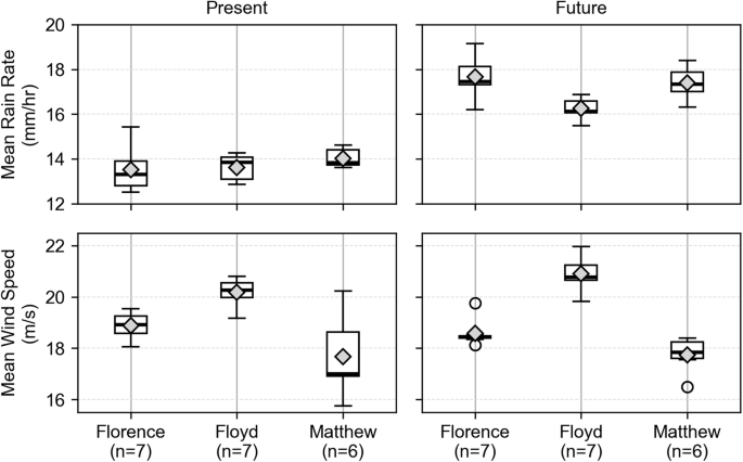
Boxplots of modeled mean rain rate (greater than 5 mm/h) (top row) and mean wind speeds (greater than 10 m/s; land values masked out) (bottom row) over a bounding box of North and South Carolina for the present (first column) and future (second column) WRF ensembles. The number of ensemble members (n) is indicated below the storm name. Within each box, a gray diamond denotes the mean of the ensemble members, a black line denotes the median, boxes denote the extent of the interquartile range (i.e., the 25th to the 75th percentile values of the distribution of the ensemble members), whiskers indicate the 5th and 95th percentile values, and circles are outliers.
The results suggest that across all three storms, the fractional change in the rain rate remains generally constant for rates greater than 5–10 mm/h (Fig. 2). The mean rain rate increases more in the future than the median rain rate. This may be a result of the higher rain rates skewing the mean to larger values while the high frequency of lower rain rates skews the median to lower values. For future realizations, we scale the present-day precipitation fields using scale factors based on the fractional difference in the mean rain calculated using a 5 mm/h minimum threshold (Supplementary Table 1). The average change in the mean wind speeds across all storms is minimal (e.g., 0.2 ± 0.5 m/s). Similarly, the average change in the minimum pressure is small, less than 1%. Of the hydrometeorological inputs used in future scenarios, we only scale the precipitation fields as the change in the mean wind speeds and minimum pressure is small.
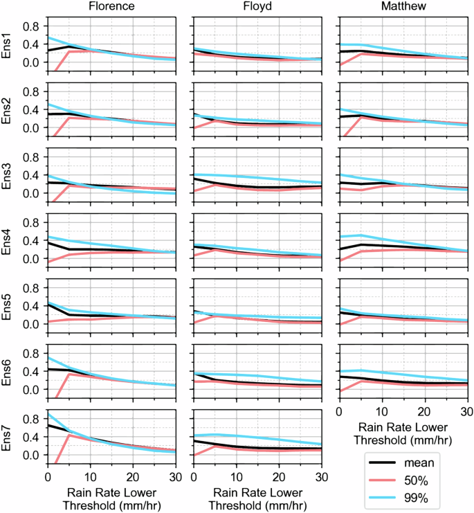
The fractional difference of the storm mean, median (50%), and 99% percentile rain rates (mm/h) in the future over the Carolinas using different lower thresholds is shown. The y-axis shows the fractional difference of the mean (black line), median (pink line), and 99% percentile (blue line) rain rates for lower thresholds ranging from 0 to 30 mm/h (x-axis).
The mean rain rate increases across the Carolinas by 31 ± 12%, 19 ± 3%, and 24 ± 4% for Hurricanes Florence, Floyd, and Matthew, respectively. While the rain rate scale factors applied to Floyd and Matthew are smaller than those applied to Florence, there is a larger increase in the areal extent of precipitation for these events34. The uncertainty range for the Florence ensemble is larger, likely because of the convective, banded nature of the precipitation in Florence as compared with the large swaths of more stratiform rainfall with Matthew and Floyd34. Because the convective rainbands are much smaller in size, the small track deviations exhibited by each ensemble member could result in large precipitation amounts falling over a region that had much less or no rainfall in another ensemble member.
To account for changes in the mean sea level in the future, we apply five sea level rise amounts to the ADCIRC water levels which are used as inputs to the coastal boundary of SFINCS for each ensemble member. We randomly sample sea level rise amounts from a uniform distribution generated using the IPCC’s AR6 regional sea level rise projections at Beaufort, NC for the SSP5-85 medium confidence scenario; the 2100 planning period corresponds to ~4 °C Celsius of warming42. The sea level rise distribution mean is 1.12 m with a 95% confidence interval of 0.68 and 1.57 m (Supplementary Fig. 1).
The total number of members in the future ensemble is 35 (7 scaled precipitation fields each with 5 probabilistic sea level rises), 35, and 30 for Florence, Floyd, and Matthew, respectively. These simulations are compared to the flooding generated in the present. Figure 3 shows the maximum flooding for each storm in the present, the mean maximum flood extent across the future ensemble, and the mean difference in water depths between the future simulations and the present simulations (the maximum difference is shown in Supplementary Fig. 2). In the future, mean maximum overland water levels for all three storms increase by 0.69 m (±0.04 m) and the 95th percentile increases by 1.14 m (±0.05 m). Specifically, the mean maximum overland water level increases by 0.71 m (±0.39 m), 0.74 m (±0.45 m), and 0.64 m (±0.40 m) for Hurricanes Florence, Floyd, and Matthew respectively.
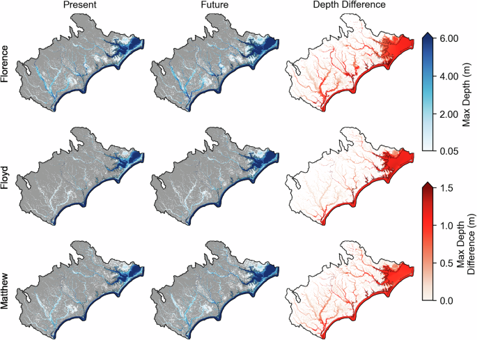
The maximum flood depths for Hurricanes Florence, Floyd, and Matthew simulated in the present climate (left), the mean of the maximum flood depths simulated across the future ensemble (middle), and the difference in flood depths between the present and future (right).
Flood driver attribution
For the present and each of the future ensemble members, we simulate total water levels in SFINCS for three scenarios: (1) coastal processes—which include coastal water level and wind boundary conditions only, (2) runoff processes—which include rainfall and streamflow boundary conditions only, and (3) compound processes—which include coastal water level, wind, rainfall, and streamflow boundary conditions. We use these model outputs to attribute flooding to the different processes based on the scenario that generated the greatest water level for each of the ensemble members. Compound processes are the primary driver of maximum water levels if the water level from the combined scenario is greater than both the coastal and runoff using a threshold of 0.05 m.
We compare the maximum water levels by driver for each future ensemble member to the flooding in the present ensemble mean for the corresponding driver – generating an ensemble of water level difference maps. From these, we compute the average difference between the modeled water levels across the entire domain which are shown in Fig. 4. We calculated the mean difference in maximum overland water levels (water bodies masked out) across the three storms attributed to coastal processes is 0.70 m (±0.03 m) and to runoff processes are 0.28 m (±0.06 m), and to compound processes is 0.82 (±0.11 m). Locations with negative values in Fig. 4 indicate that the primary driver of flooding shifts from coastal or runoff to compound or in some cases, that the primary driver shifts from compound in the present to coastal in the future. The shift from individual to compound drivers is largely due to increases in sea level which produces coastal flooding further inland than in the present where runoff processes occurred in isolation in inland areas. There are few areas where the driver shifts from compound to coastal and this primarily occurs in the estuaries and sounds (e.g., behind the barrier islands). In these areas, runoff processes are negligible when compared to coastal processes because of the effects of sea level rise (average of 1.12 m increase in mean sea level) on inundation.
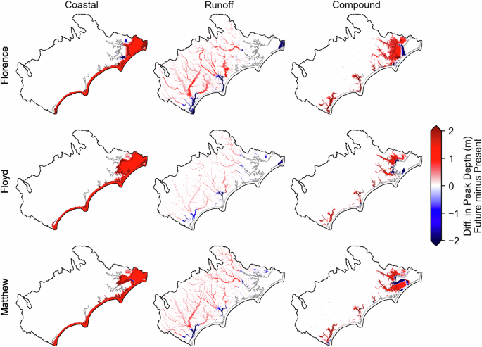
Areas where there is an increase in flood depth in the future for a given process are shown in red and a decrease is shown in blue. In the present, the maximum water levels in the lower portions of the major rivers are primarily driven by runoff processes but in the future, they are driven by compound processes as this area shifts inland due to sea level rise.
For each present and future simulation, we calculate the maximum overland flood extent (water bodies masked out) across the domain and attribute it to one of three processes: coastal, runoff, or compound. The relative contribution of each process to the total flood extent was computed using the ensemble mean water levels for each storm. The result is shown in Fig. 5. The average overland flood extent across the three storms in the present is 66,110 sq. km. (±880 sq. km.) and in the future is 66,960 sq. km. (±510 sq.km.). This equates to a 1.3% (±0.7%) increase in total flood extent between the present and the future. Runoff processes are the largest contributor to overland flood extent both in the present (94 ± 1.1%) and in the future (90.7 ± 0.9%) across all three storms. While the overall flood extent does not change significantly between the present and the future, the relative contribution of compound and coastal processes increases (2.6 ± 0.5% and 1.1 ± 0.7%, respectively) while the contribution of runoff processes decreases (−3.7 ± 0.2%). For Florence, most of the areas where runoff processes dominated shift to compound processes whose relative contribution increases by 3.4%. For Floyd, the relative contribution of runoff processes decreases by 4% as compound and coastal processes increase by 2.2% and 1.8%, respectively. For Matthew, the relative contribution of runoff processes to total flood extent decreases by 3.5% as compound processes increases by 2.3% and coastal processes increase by 1.2%. While the increase in the contribution of compound flooding to the total flood extent in the future is relatively small compared to runoff, the area exposed to compound processes increases by two-thirds relative to the present (64.5 ± 7.7%). Similarly, the area dominated by coastal processes increases by 145% and 120% for Floyd and Matthew, compared to Florence where it only increased by 10%. A boxplot of the maximum overland flooded area (sq. km.) attributed to each driver and the total flood extent using all ensemble members is shown in Supplementary Fig. 3.
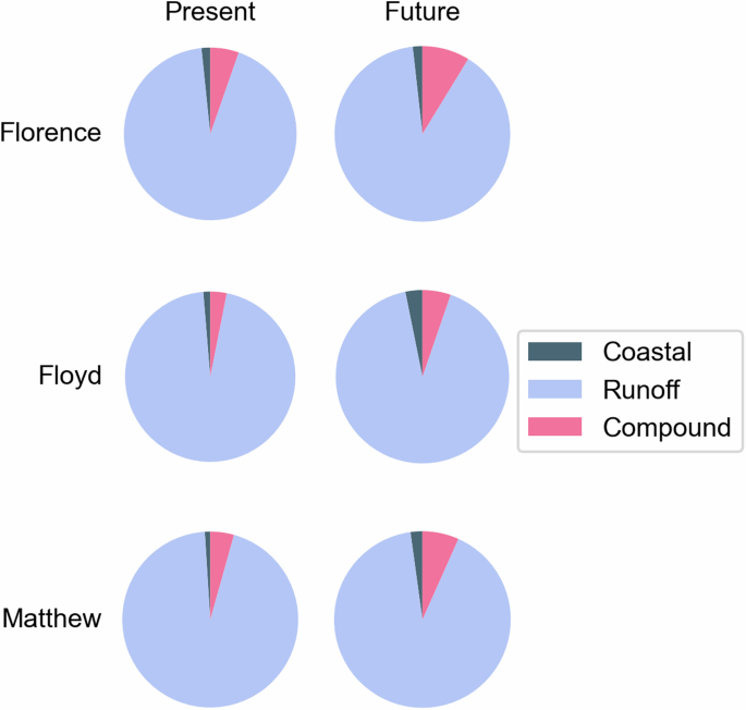
Runoff is the primary contributor to flooding across the domain in the present and future, however the relative contribution of compound and coastal flooding increases in the future for all storms.
Compound flooding
The contribution of compound processes to maximum flood extent and total water levels increases in the future across the three storms. This indicates the importance of simulating both runoff and coastal processes and their dynamic interactions when assessing TC flood hazards and exposure. Figure 6 shows the spatial extent of maximum flooding from compound processes in the present simulation compared to the maximum extent across the future ensemble members. The maximum extent of compound flooding in the future for each storm compared to the present is shown in the first column of Fig. 6. A grid cell is included in the maximum extent of compound flooding if maximum total water levels were attributed to compound processes in at least one of the future ensemble simulations. In the second column of Fig. 6, we show the frequency the maximum water level in a grid cell is attributed to compound processes across the ensemble. Across all storms, there is an expansion of compound flooding inland (e.g., upriver) as well as an increase in the width of the floodplain along the major rivers, estuaries, and sounds. Coastal rivers such as the Cape Fear near Wilmington (Fig. 6) have a high likelihood of compound flooding in the future regardless of the amount of sea level rise. Zoomed-in extents of the other major parts of the coastline are shown in Supplementary Figure 4 including Myrtle Beach, New Bern, Greenville, and the Down East area.
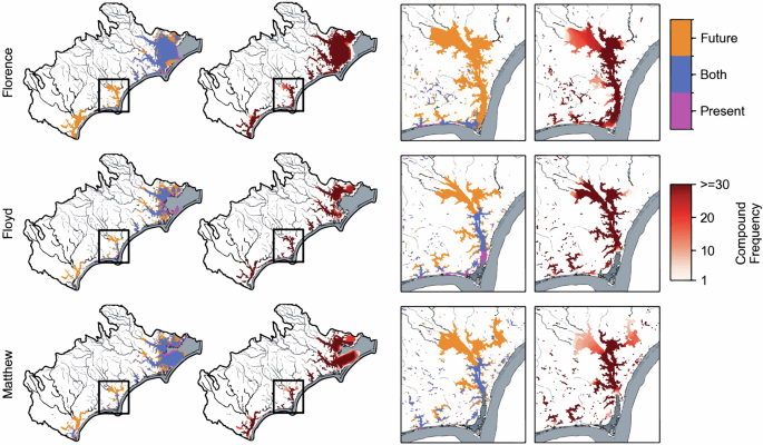
Areas flooded by individual processes (e.g., rainfall, coastal) are not plotted. The entire domain is shown in the top panel and the black rectangle highlights the location of the Wilmington metropolitan area which is shown in the bottom panel. Present-only is in pink, future-only is the maximum extent of compound flooding across the full ensemble in orange, and both present and future is in blue. Darker red colors indicate a higher probability of compound flooding occurring in the future across all ensemble members. In the future, the model results show an expansion of compound areas further inland and a widening of the floodplain for all three storms.
Discussion
In this study, we demonstrate the application of an ensemble of scale factors and probabilistic sea level rise to estimate changes in compound flood hazards for three historic TCs with unique tracks and intensities. We leverage outputs from a high-resolution atmospheric model to calculate scale factors which are applied to analyzed data enabling our flood simulations to have spatially and temporally consistent hydrometeorological inputs across climate scenarios. We simulated flooding from three TCs over a large area that includes multiple watersheds. This enables a comparison of inland and coastal TC flooding across multiple storms and varying topography (e.g., low-gradient coastal plains, inland areas with incised channels) whereas previous studies have focused on a single event or catchment. Our approach generates flood hazard information that considers the uncertainty in the projected changes to TC drivers of flooding (e.g., precipitation, sea level rise) that can be used to better link changes in the climate directly to changes in flood exposure. Our method can be replicated with community-scale modeling frameworks which are used to inform local engineering standards and flood mitigation policy.
The impacts of climate change on TC characteristics are not uniform across all storms. The mean rain rates, wind speeds, and minimum pressure across the Carolinas scaled similarly to the changes along the entire storm track. For example, we find that the mean rain rate (considering those >5 mm/h) increases across the Hurricane Florence ensemble by 31 ± 13% compared to the Floyd and Matthew ensembles which increase by 19 ± 3% and 24 ± 4%. In the future, TC mean wind speeds (greater than 10 m/s; land masked out) increased in magnitude by 0.5% across the entire storm track and their relative frequency increased by 3.9%. In contrast, we found that when analyzing changes in mean wind speeds over the Carolinas, they increased by 1.4% and their relative frequency decreased by 2.8%. These findings have implications for selecting appropriate scale factors (e.g., assuming Clausius-Clapeyron would overestimate the precipitation scaling for Matthew and Floyd, track averaged change in wind speeds would underestimate wind influence along the Carolinas) and highlight the need for high-resolution, detailed investigations into how TCs interact with the land surface and meteorological systems inland.
With 4 °C of warming, the relative contribution of compound flooding to the total flood extent increases by more than 2% for Hurricanes Florence, Floyd, and Matthew. Compound flooding expands inland, moving upriver and beyond the existing floodplain. This is a result of the interaction between larger river discharges (e.g., increased precipitation) and coastal processes that reduce the effective capacity of the system to drain (e.g., sea level rise). The overland areas associated with compound flooding increase on average by 1800 ± 380 sq. km (64.5 ± 7.7%) which is roughly the size of the New Bern, NC metropolitan area and 1.5 times the size of the Wilmington, NC metropolitan area. Notably, these areas are exposed to flood depths 0.82 m (±0.11 m) greater than in the present simulation. Overland areas where coastal processes dominated experienced increases in mean depths by 0.70 m (±0.03 m), slightly less than compound areas. There is a small reduction (3.7%) in the contribution of runoff processes to maximum flood extent in the future as runoff-only areas become exposed to coastal processes, shifting their primary driver in the future to compound or coastal processes. Despite this, runoff processes remain the largest contributor to maximum overland flood extent (>90%) and these areas had an average increase in flood depths 0.28 m (±0.06 m). The increased depths as a result of the three flood processes have implications for both infrastructure damage but also potential disruptions due to longer durations of inundation impacting response and recovery.
Across the three storms, the overland flood extent increases in the future (average of 850 sq. km.), primarily in the areas that are very flat where compound and coastal processes dominate (e.g., between 10 and 15 m NAVD88). The expansion of the floodplain inland in runoff dominated areas is negligible at the domain scale because of natural levees and steeper topography, however at a local scale (e.g., community), changes may be significant and impactful. The flooded area for Hurricane Florence and Floyd increases significantly more in the future compared to Matthew (Supplementary Fig. 3). For Florence, this increase is primarily occurring along the NC and SC border in the southern portions of the model domain where rainfall is concentrated. In these areas, runoff processes were the primary contributor to maximum water levels in the present due to heavy precipitation that generated pluvial and riverine flooding that exceeded storm surge levels. In the future, sea level rise will introduce coastal processes to these areas that cause a shift in dominant flood processes to compound. While the increase in the mean rain rates for Hurricanes Matthew and Floyd is smaller, they both generated a larger areal increase in precipitation over the middle of the domain that increased runoff across all watersheds which led to the expansion of compound flooding in all rivers across the domain (Fig. 5). While Matthew and Floyd are not often thought of as events that generate compound flooding, our results suggest that they did and that under future warming conditions, the relative contribution of compound flooding along the coast would be much greater in similar storm events. Similarly, Hurricanes Matthew and Floyd had a much larger increase in the contribution of coastal processes to the maximum flood extent compared to Florence which is likely due to the storm tracks and the interaction between sea level rise and wind patterns.
In conclusion, we demonstrate that the contribution of compound flood processes to flooding will increase due to increased mean sea level and precipitation, shifting the area were coastal and runoff processes interact upriver and outside the floodplain. This pattern occurs for TCs that are not typically thought of as generating compound floods highlighting the importance of modeling dynamic interactions for all TCs. However, our approach requires the availability of multiple high-resolution models to capture the interaction of flood drivers and processes in detail, which can be computationally intensive and requires bringing together multiple disciplines. Future work should seek to understand what model-related simplifications can be taken to reduce the number of simulations (e.g., ensemble mean vs full ensemble) and complexity while maintaining enough detail to understand the complex interactions between physical processes. Importantly, our assessment of the relative contributions of coastal, runoff, and compound processes expands beyond coastal areas (e.g., <20 m NAVD88), traditionally the focus of TC flood hazard assessments. In doing so, we demonstrate that runoff processes dominate the overall flood extent across all three TCs. While considering the interaction of coastal and runoff processes at lower elevation is important to quantifying changes in future exposure, simulating the full extent of runoff-driven flooding is critical to TC risk assessments and should not be neglected.
Methods
Scale factors
We compute scale factors using the fractional difference between the WRF present and future ensemble member simulations where the ensemble members are equally weighted. The WRF tracks and their variation across the Carolinas are shown in Supplementary Fig. 5. For the rain rates, we subset the data to the rain that fell over the Carolinas (see Supplementary Fig. 6) to compute the empirical cumulative distribution function (ECDF) using minimum rain rate thresholds between 0 to 30 mm/h, binning the data at 5 mm/h increments. From the ECDF (Supplementary Fig. 7), we extract the mean, 50% (e.g., median), and 99% percentiles and calculate the fractional difference between the present and future for each ensemble member. We repeat this analysis using the WRF wind speeds (masking out land areas) and minimum pressure over the Carolinas and across the entire WRF domain. We find that the fractional difference between the mean and median wind speeds (Supplementary Figs. 8 and 9; Supplementary Table 2) and minimum pressure (Supplementary Figs. 10 and 11) are similar and generally constant across all thresholds for each storm. While we acknowledge that a decrease in pressure can impact storm surge height, we assume that such a small change (-0.9 ± 0.4%) would have a negligible impact on the storm surge simulated in ADCIRC.
Atmospheric model
TC rainfall, wind, and pressure fields were simulated using the Weather Research and Forecasting (WRF) model version 4.2.241.To represent future storm environments, the PGW approach was used31,43. 100-yr temperature change fields (“deltas”) were computed using an ensemble of global climate model outputs from high-emission scenarios (RCP8.5, SSP5-85) from the Coupled Model Intercomparison Project (CMIP) 5 for Hurricanes Matthew and Floyd and CMIP 6 for Hurricane Florence. The deltas, which were calculated for soil temperature, air temperature, skin temperature, and sea surface temperature, were used to adjust the initial conditions of the present climate simulations of Hurricanes Florence, Floyd, and Matthew. For each storm, an ensemble of model runs with varying physics options are generated to compare precipitation characteristics for the three storms. Hurricanes Florence, and Floyd have an additional ensemble member compared to Matthew (which has 6) to consider another microphysics scheme which is discussed in more detail in Hollinger Beatty et al.34. These cases were selected because of their impact on North Carolina, and because they took place in diverse synoptic environments. The simulations are run with a parent domain with 12-km grid spacing, and a high-resolution nested domain over the southeast U.S. with 4-km grid spacing to allow convection to be represented on the grid (Supplementary Fig. 6). A more detailed overview can be found in Hollinger Beatty et al. 34. In the future, all storms exhibited a larger total accumulated rainfall, higher rain rates, and larger areal coverage of rain rates exceeding specific thresholds across the Carolinas. Hourly gridded wind and rainfall WRF outputs are used in this study and 6-h pressure fields are interpolated to an hourly interval along the simulated storm tracks.
Ocean-to-coast circulation model
Coastal water levels (e.g., tides, surge) were simulated using the two-dimensional (2D) depth-integrated version of the ADCIRC model44,45. The model has been compared to observational data and used for retrospective analyses46,47,48, hazard evaluation49 and other applications. The unstructured computational mesh that is used in this study covers the North Atlantic basin and was adapted from previously validated meshes50. The mesh resolution along the Carolinas coastline is ~50 m, 1 km along the continental shelf and around 5–10 km in the deep ocean. For each storm, eight tidal constituents were obtained using OceanMesh2D51 and incorporated into ADCIRC as periodic boundary conditions at the ocean boundaries of the mesh for the three events.
The initial water level for all ADCIRC runs was set to 0.13 m MSL which has been configured in validation simulations of Hurricanes Matthew and Florence previously50,52. A tidal spin-up of 14 days before the storm is used to generate the initial ocean conditions for each storm. For the storm runs, we initialize the model with the spin-up and apply hourly WRF winds and pressure fields to the mesh. ADCIRC outputs water levels every 10-min at 713 points located along and near the coastal boundary of the SFINCS model. We extend the ADCIRC simulation beyond the length of the storm (and WRF output) to generate tidal water levels to apply to SFINCS which is run for a longer duration to allow the TC runoff to fully drain across the domain. For each storm, we complete a tide-only simulation of water levels that is used as the boundary condition for the runoff scenarios in SFINCS where no storm surge occurs.
We visually compared ADCIRC water levels against NOAA tide gauges across the model domain to confirm the wind and pressure fields used were generating observed water levels. We show examples of this comparison at four locations in Supplementary Fig. 12. Sea level rise in the future scenarios is superimposed to the ADCIRC coastal water levels before being applied to SFINCS. ADCIRC is computationally expensive to run and the difference in the modeled water levels along the SFINCS boundary was minimal when sea level rise was incorporated directly into the ADCIRC simulation versus linearly added to the output (Supplementary Fig. 13).
Flood inundation model
Total water levels were simulated across the Carolinas using the 2D raster-based hydrodynamic model SFINCS39. The model solves simplified equations (e.g., Local Inertial without advection or Simplified Shallow Water Equations) and employs a subgrid approach that enables it to efficiently compute overland flooding at a coarse resolution while maintaining finer resolution information on topography and land cover. The gridded model domain used in this study covers an area ~77.6 thousand square kilometers, including five major watersheds, and has been previously validated for Hurricanes Florence and Matthew53. The modeled water levels are output at the grid resolution of 200 m and are downscaled to a subgrid resolution of 5 m. The model uses 30 m resolution data to parameterize overland flow roughness and infiltration (e.g., Curve Number method with recovery). We use the 2016 National Land Cover Data (NLCD) 2016 Land Cover for all present and future simulations. A more detailed overview can be found in Grimley et al53.
For the hindcast simulations of Florence and Matthew, we used NOAA’s Multi-Radar Multi-Sensor (MRMS) Quantitative Precipitation Estimate gridded rain-gage adjusted, radar-rainfall data which has an hourly temporal resolution and 1 km spatial resolution. We use Ocean Weather Inc. (OWI) wind and pressure fields for Matthew and an OWI-adjusted product for Florence50 with a spatial resolution of 0.05° (~5.0 km) and a 15-min temporal resolution. For Floyd, we use hourly wind and rainfall data from the European Centre for Medium-Range Weather Forecasts ERA5 data which is a global reanalysis with a spatial resolution of ~28 km. Rainfall and wind fields are applied directly to the SFINCS model grid. ADCIRC 20-min modeled water levels at 713 points are interpolated to the SFINCS grid cells at the coastal boundary. For both the present and future simulations, we use observed river discharge from nine USGS gages as inflows to the upstream boundary for Florence and Matthew (only six available for Floyd). These inflows are located just downstream of managed reservoirs, and we assume the operation of these structures in the present day is unchanged in the future. There are processes that we have simplified including stationary land cover, constant antecedent soil moisture, and assuming consistent reservoir operations in the future. Specifically, we recommend that future studies investigate the role of topobathymetry (e.g., shape and orientation of estuaries) and watershed size (e.g., time of concentration) on the extent of compound processes.
Because of the computational efficiency of the model, we simulate three scenarios, toggling on and off different forcings, to isolate the impacts of the different inputs on total water levels. For the runoff scenario, we simulate the gridded precipitation fields and USGS streamflow to the upstream boundary with a tides-only water level as the downstream, coastal boundary. For the coastal scenario, we run the model and only apply the ADCIRC modeled water levels and WRF gridded wind directly to the model grid alone. For the compound scenario, we run the model using wind and precipitation, USGS discharge, and ADCIRC water levels to the model. The SFINCS simulation of Florence was 17 days (2018-09-13 to 2018-09-30), 8 days for Matthew (2016-10-07 to 2016-10-15), and 8 days for Floyd (1999-09-14 to 1999-09-22).


Responses