Climate change reduces the wind chill hazard across Alaska

Introduction
Wind chill temperature (WCT), which accounts for not only temperature but also wind speed, is used in assessing the risk levels for outdoor activities in cold-weather conditions. Initially designed to measure human comfort, the WCT was refined by the National Weather Service (NWS) to offer a more precise index of cold sensations1,2,3. Joint exposure to low temperature and high wind speed can lead to severe cold weather illnesses such as frostbite and hypothermia4,5. For instance, humans may expect a degree of discomfort and potential risk of frostbite over extended time exposed to ambient air temperature below −15 °C; however, when the wind speed reaches 48 km per hour, the risk of frostbite for most people increases markedly within 30 min of exposure2. Importantly, there is also a strong correlation between WCT and life-threatening diseases such as those related to the heart, cardiovascular, and respiratory systems6,7. One report showed that two-thirds of weather-related mortality among United States residents from 2006 to 2010 were attributed to excessive natural cold8. A study specifically of Arctic populations found associations between colder climate and a range of mortality, morbidity, and fertility indicators, indicating that risks are not restricted to areas less historically adapted to cold weather9. To protect the public from the dangers of wind chill, the NWS issues wind chill advisories, watches, and warnings to alert people to the real threats to their daily lives and health10,11.
Alaska is one of the coldest regions in the world that has been settled and inhabited by humans12. However, the region has also experienced the largest recent increase in annual average temperature in the United States13, with warming exceeding 2 °C since the mid-20th century14. This ongoing warming trend poses challenges for both residents and environments in the state. To project these changes, many studies have explored the future changes in Alaska’s climate with global climate models (GCMs) part of the fifth or sixth phase of the Coupled Model Intercomparison Project (CMIP5 or CMIP6), finding that air temperature in the state is projected to increase at a faster pace than global average temperatures over the 21st century15,16. Over the same period, there is some evidence that wind speed may increase in the cold season and decrease in the warm one17. Given that the temperature is projected to increase, the wind speeds are eventually expected to weaken across the state18. Moreover, these rising temperatures contribute to increased risk of natural hazards such as permafrost thawing, flooding, landslides, and erosion; therefore, the new term “climigration” has been coined to describe the ongoing and future migration of Alaskan communities19. However, while the projections of air temperature and wind speed have been examined as individual variables, little is known about their combined impacts in terms of WCT, which provides basic information toward improved adaptation and mitigation plans.
To address questions about changes in WCT across Alaska, we need high spatial resolution climate model outputs because the state has complex orography with a large elevation range (0–4690 m) and small-scale variability of near-surface wind. Here we use the Weather Research and Forecasting (WRF) model20,21, which provides meteorological variables with a high spatial and temporal resolution (see Methods) and has been widely used for hydro-climatological applications22,23,24. To assess future climate changes, we use the pseudo-global warming (PGW) approach, in which the boundary conditions of a regional climate model for the current climate are perturbed to reflect possible changes in large-scale mean-state climate conditions. A key advantage of the PGW method is that it avoids introducing model biases due to the direct downscaling of climate model data. The current and future simulations also have very similar internal variability, which largely reduces the impact of this variability on our climate change results25,26. A downside of the PGW method is that it only partly captures forced circulation change27. While mean-state circulation change is included, any forced change in circulation anomalies (i.e., changes in synoptic-scale circulation variability) is not considered. The importance of changes in circulation anomalies, however, varies regionally, and there is evidence that for wintertime in Alaska contributions from circulation anomalies may be small27. The PGW method has been recognized for its computational and data storage efficiency, flexibility in designing future projections, and agreement with the traditional dynamic downscaling technique when implemented adequately28,29,30,31.
Future projections in WCT across Alaska can reveal important characteristics of natural hazards, particularly their frequency and timing under extreme conditions. Here, we focus on two aspects of wind chill conditions: the frequency of extreme events and their timing. These factors indicate whether the overall hazard magnitude is expected to change, when to be concerned, and if the seasonality is shifting—potentially requiring updates to preparation plans. In addition, it is important to understand whether these hazards occur throughout the year or are concentrated in specific months, as this can impact many parts of the natural system, including human health, energy use, ecosystem, and population migration32,33,34. Official NWS extreme cold warning and advisory criteria are set locally. In Alaska, a wind chill advisory is issued when the WCT begins to drop below −30 °F (−34.4 °C)35. Therefore, we explore the projected changes in extreme wind chill days (EWCD; i.e., days with WCT <−34.4 °C) across Alaska, using the PGW method with WRF simulations.
Results and discussion
Changes in the frequency of EWCD
To shed light on the frequency changes in the EWCD, we first compute the annual average occurrence frequency of EWCD from both Control (CTRL) and PGW simulations, together with their differences (i.e., PGW-CTRL) (top panel in Fig. 1). The EWCDs occur up to 150 days or more per year (i.e., more than 40% of the year) during the historical period, with higher values in areas of higher elevation and toward the northern part of the state. The results of the PGW simulations point to a decrease in EWCD under warming conditions, with an overall decrease across the state ranging from a decrease of less than a week to more than two months. Due to the relationship between a reduction in EWCDs and topography (Supplementary Fig. 2), we examine the dependence of these changes on elevation (Supplementary Fig. 3). High-elevation regions in Alaska are expected to experience relatively small changes (i.e., less than 20%) and some of these areas are expected to continue experiencing a high frequency of EWCD. On the other hand, the largest changes are expected to occur in lower elevation areas, with a relative change of over 50%, especially in the northern and western coastal areas. To investigate how many people are expected to be impacted under global warming conditions, we analyze changes in EWCDs across different elevation ranges in terms of impacted population. As shown in Fig. 1, about 60% of the state’s population resides in lower elevation areas (i.e., up to 100 m above sea level (m.a.s.l.)), which is also the range expected to experience the largest reduction in EWCDs (median reduction of 43 days/year). Approximately 32% of the population lives between 100 and 400 m.a.s.l., with a median reduction in EWCD of 30 days per year when averaged over the future time period. Thus, many of Alaska’s residents are expected to experience a decrease in extreme wind chill conditions of more than a month per year under the PGW scenario.

a The annual average of EWCD across Alaska is shown for the CTRL simulation (left panel on the top) and the PGW simulation (middle panel on the top), with the difference between PGW and CTRL (i.e., PGW-CTRL) shown in the right panel on the top. These differences are statistically different from zero at the 5% level across the vast majority of the state, with the exception of the locations in Supplementary Fig. 1. b The boxplots in the bottom-left panel show the projected reduction of EWCD across different elevation ranges, using the 5 and 95% percentiles to represent the lower and upper limits. To the right, the pie chart to its right displaying the corresponding population percentage.
Main driver of extreme wind chill conditions
To identify whether changes in air temperature or wind speed drive the future changes in EWCD, we consider two scenarios for calculating WCT in the PGW simulation (Fig. 2): (1) using air temperature from CTRL and wind speed from PGW (referred to as “PGW_WS”); and (2) using air temperature from PGW and wind speed from CTRL (referred to as “PGW_T”). If the differences in Fig. 1 are more similar to what is observed in the PGW_WS (PGW_T) scenario, then we can conclude that wind speed (temperature) changes are more responsible for our results. This experimental design is possible due to the similarity in day-to-day synoptic weather in the control and PGW simulations. Compared to the results with the original PGW simulation (i.e., PGW_Full; left panel in Fig. 2), the results based on PGW_WS show a completely different pattern, with a much more muted reduction and an overall increase in EWCDs due to the increases in wind speed during the cold season. The results of PGW_T, on the other hand, closely resemble the differences between CTRL and PGW experiments both in terms of spatial patterns and magnitude. Therefore, we conclude that future changes in the frequency of EWCDs in our experiments can be attributed to changes in air temperature, which play a much stronger role than wind speed. We interpret this conclusion within the limitation of the PGW approach in not allowing for the possibility of forced changes in synoptic circulation variability. Quantifying the role of forced change in circulation anomalies for EWCDs demands large ensemble climate simulations to overcome sampling issues36 that are currently unfeasible with km-scale models. Our conclusion is, therefore, based on the assumption that synoptic eddy contributions to EWCDs are small compared to contributions from mean-state changes.
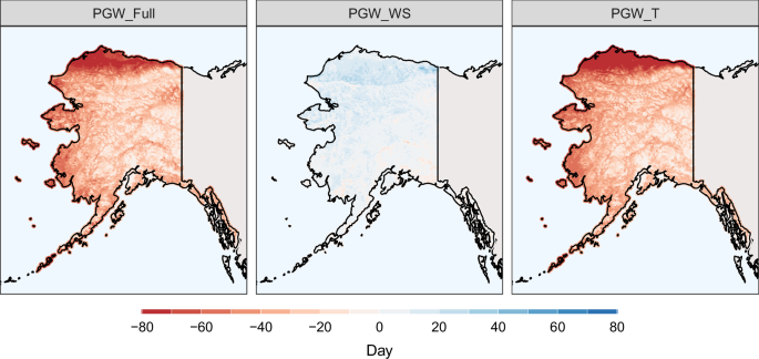
Each panel shows the difference between PGW and CTRL (i.e., PGW-CTRL) for the three PGW scenarios. “PGW_Full” refers to the original PGW simulations (both wind speed and temperature from PGW simulation; see the top-right panel in Fig. 1). The “PGW_WS” scenario uses wind speed from PGW and air temperature from CTRL, while “PGW_T” uses air temperature from PGW and wind speed from CTRL.
Changes in timing of EWCD
To capture the changes in the timing of EWCD occurrences, we use the mean direction to represent the average timing of EWCD occurrences and the mean resultant length to indicate the intensity (see Methods). Figure 3 shows the average timing of EWCD occurrence and intensity from the CTRL and PGW conditions, and their difference (i.e., PGW-CTRL). During the historical period, the average timing is primarily concentrated in the winter, while it mostly shifts to early spring in the interior and northern Alaska under future climate conditions. The difference in the mean direction indicates the timing of EWCD is expected to be delayed by at least 1 week and possibly up to three weeks across much of Alaska; at the same time, seasonality is projected to become more concentrated. As shown in Supplementary Figs. 4, 5, even though the overall number of EWCDs is projected to decrease, we also see a redistribution of these events between CTRL and PGW: January is the month with the largest contribution to the annual totals in the CTRL simulations, while EWCDs in January and March tend to dominate in the PGW scenario, explaining the identified changes in the seasonality of this hazard.
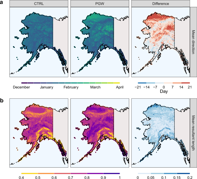
a The average timing of the EWCD occurrence (represented by the mean direction; top panel) for CTRL (first column) and PGW (second column) simulations. The difference between PGW and CTRL (i.e., PGW-CTRL) is shown in the right column. The legend for the difference in mean direction is in days. b The average intensity of the EWCD occurrence (represented by the mean resultant length; bottom panel) for CTRL (first column) and PGW (second column) simulations. The difference between PGW and CTRL (i.e., PGW-CTRL) is shown in the right column.
To verify that the changes in EWCD timing are consistent with the main drivers that have influenced the EWCD frequency, we perform the same analyses for the PGW_WS and PGW_T scenarios (see Supplementary Figs. 6, 7). The results support the major role of air temperature, with the PGW_T scenario closely resembling the PGW experiments in both spatial patterns and timing of EWCD occurrences; on the other hand, the PGW_WS scenario shows no major difference in the mean direction and resultant length compared to those observed in the CTRL (Supplementary Figs. 6, 7). Combining the changes in the timing and variability of EWCDs together with their frequency, we find that these extremes, on average, are projected to occur later in the year, during a narrower time window, and less frequently; therefore, while this hazard tended to be more chronic in the past (i.e., occurring more frequently and during a longer time window), it is expected to become more acute (i.e., less frequent and concentrated during a shorter time window) under warming conditions.
Impact of extreme wind chill conditions on communities in response to warming
Here we focus on examining projected changes in EWCD across Alaska. Our findings reveal a robust reduction in EWCD, along with a change in its seasonality. More specifically, the number of EWCD is projected to decrease, especially at lower elevations, and to become more episodic in the late winter or early spring in the future. Moreover, these detected changes are largely driven by increasing air temperature. Given that there is clear evidence that Alaska is expected to be warmer in the future14,37, our results indicate that these rising temperatures may reduce Alaska’s exposure to extreme wind chill. While it may be challenging to recognize the upside of warming in cold regions, there are some benefits, albeit limited, such as the potential development of shipping, logistics, distribution, and energy industries through the opening of new shipping routes and access to new areas for resource exploitation, including offshore oil extraction38,39. In light of this, our findings could present a silver lining to some Alaskan communities, including mitigating the risk of wind chill to provide a more comfortable environment both indoors and outdoors, reducing energy demand for heating, stimulating outdoor activities that could impact the local economy, and decreasing the risk of cold weather injuries and illnesses.
Admittedly, emphasizing only the positive aspects offers one side of the discussion as the negative impacts of a warming climate can be far more serious. One of the most serious impacts on both people and the environment in Alaska is permafrost thawing40. This degradation can cause land-surface instability and subsidence, leading not only to infrastructure damage (e.g., the collapse of buildings and bridges)41, but also to the emergence of diseases due to melting in the Arctic (e.g., bacterial activation and exposure to accumulated hazardous chemicals)42,43. In short, theses environmental threats are linked to the fact that Alaska faces a range of anticipated hazards, including natural threats such as floods, erosion, and wildfires44 as well as public health risks like the spread of infectious diseases45. Therefore, it is not surprising these environmental changes threaten community infrastructure. However, there are compelling examples of proactive climate adaptation underway to manage inevitable changes. These efforts have been made with a comprehensive understanding of the risks and opportunities of climate change, addressing regional concerns such as sea level rise, flooding, water distribution, and transportation systems in several states of the United States46. Furthermore, clear information about the magnitude and timing of climate change can help foster better coordination, communication, and knowledge sharing in the decision-making process. Taking this as a lesson, we believe that our findings, which highlight a positive aspect of warming and investigate changes in magnitude and timing of extreme hazards, can be a starting point for adapting to the challenges of climate change within Alaskan communities.
Methods
WRF data and climate simulations
We use data produced by 4 km grid spacing Weather Research and Forecasting (WRF) model version 3.7.1 simulations47. A detailed description of the model and domain setup of the CTRL simulation is presented in ref. 20. Initial and boundary conditions for the CTRL simulation are derived from the European Centre for Medium-Range Weather Forecasts (ECMWF) interim reanalysis (ERA-Interim48).
The concept of PGW simulations is expressed with a simple mathematical term defined as (mathrm{PGW}=mathrm{CTRL}+{rm{Delta }}), where CTRL and PGW respectively represent the sea surface and boundary conditions of two regional climate model simulations of the past and future climates, and Δ represents the future changes25. The PGW simulation uses the same 6-hourly ERA-Interim boundary conditions as the CTRL run with a monthly mean ({rm{Delta }}) for temperature, wind, moisture, and geopotential height. These ({rm{Delta }}{rm{s}}) are based on an ensemble of 19 global climate models from the Coupled Model Intercomparison Project (CMIP5)49. They are derived from the difference between 2071–2100 compared to 1976–2005 under the RCP8.5 scenario50. More details about the PGW simulation can be found in ref. 21. We note here, however, that the ({rm{Delta }}{rm{s}}) are changes in the mean climate, and we, therefore, do not consider the possibility of forced changes in circulation anomalies. The CTRL and PGW simulations cover a 12-year period from 2003 to 2015, excluding 2004 because of data gaps during that year. While there may be some sensitivity to our use of ERA-Interim and CMIP5 compared to the more recent ECMWF Reanalysis v5 and CMIP6, our main findings of the directional change in WCT, relative importance of temperature versus wind, and general spatial patterns of change relative to terrain will likely not change.
In our analysis, we calculate WCT generated by two simulations: one for past climate conditions (i.e., CTRL) and the other for a future climate scenario (i.e., PGW), enabling us to quantify the projected changes in wind chill conditions. We use air temperature and wind speed data from the WRF simulation to calculate WCT as described in the following section. The quality of simulating past air temperature with this model was previously evaluated and robustly represents Alaska’s climate20. While past wind speed simulations with the WRF model were shown to perform well for hydrometeorological applications51, this validation was done only for Alaska’s offshore regions and not for the state’s interior. Overall, the validation of wind simulations in regions like Alaska is extremely limited because of the challenges associated with the sparse data availability, and this is something to keep in mind when interpreting these results. However, the predominance of populations living in lower-elevation coastal locations lends confidence in the validity of our findings with respect to human health impacts.
WCT and EWCD
WCT is calculated as a combination of air temperature and wind speed, as originally formulated by Eq. (1)2:
where ({T}_{{air}}) is air temperature at 2 m above the surface in Fahrenheit and UV is wind speed at 10 m above the surface in miles per hour. The WRF data provide these variables at an hourly temporal resolution. Once the wind chill temperature is obtained in Fahrenheit, we convert it to Celsius. We apply this equation to analyze EWCD across Alaska, defining EWCD as days with a WCT of −34.4 °C or lower for at least 1 hour.
Population data
We use a high-resolution population distribution data from LandScan Global 2022, developed by Oak Ridge National Laboratory52. The LandScan Global dataset offers high-resolution global population distribution, representing an ambient (24-hour average) population at a 1 km spatial resolution.
Circular statistics
Many studies have applied circular statistics to describe the signal of temporal changes in the circular nature of climatological data such as floods53,54,55 and precipitation56.
Circular statistics begins with converting standard data to circular data using unit radians. The advantage of circular statistics is that it converts temporal attributes into angular values, so it can effectively analyze daily or seasonal characteristics and their occurrence patterns57,58. In addition, circular statistics can provide descriptive and inferential skills suitable for circular data using the averaged location and concentration that climate events have occurred in a cycle. Following the approach of Magilligan and Graber57 and Pewsey et al.58, for example, if the data consist of days of the year (i.e., Julian dates, day 1 to day 365), day (i) can be converted to an angular degree (theta), a value between 1° and 360°, given by Eq. (2):
This angular degree (theta) is then converted to radian, ranging from 0 to (2pi). Consequently, the magnitude of the angle corresponds to the number of values on that day.
The mean direction and mean resultant length are commonly used to measure location and concentration, respectively. For the circular data, each date is represented by a vector with a unique direction and magnitude. The mean direction represents the central location of the circular data. The mean direction (bar{theta }) can be given by Eq. (3):
where (n) is a sample size, ({theta }_{i}) is Julian date in angular degrees for a given observation (i).
The mean resultant length (bar{R}) indicates how closely the data points are clustered around the mean direction. It reflects the strength of the mean for each date and is calculated from vectors with unit magnitude. The mean resultant length (bar{R}) can be given by Eq. (4):
The (bar{R}) value is a measure of seasonality: an (bar{R}) value closer to 1 means that the data are clustered around the mean direction, indicating a stronger seasonality, while an (bar{R}) value closer to 0 means that the data points are evenly distributed around the circle.


Responses