Climate driven generative time-varying model for improved decadal storm power predictions in the Mediterranean

Introduction
Decadal timescales have emerged as vital planning horizons for governments, businesses and society, offering an attractive tool for short-term climate change adaptation and mitigation planning1,2. Despite this recognition, relevant gaps persist in our understanding and prediction of precipitation patterns, particularly at regional scales, representing notable deficiencies in climate science3,4. Extreme rainfall events, in particular, pose relevant threats, regarded as one of the most damaging climate hazards5, raising concerns about their changing frequency and intensity6. In this context, advancing the central role of extreme weather events prediction and information, which is closely embedded in climate dynamics7, is a critical contribution to achieving the Sustainable Development Goals8.
Storm-power indicators effectively support climate prediction and guide landscape conservation planning efforts9. Moreover, historical and statistical climatology plays a crucial role in understanding how the Earth system responds to such climate forcing mechanisms. Rainfall erosivity is pivotal in informing the development of conservation and environmental management plans in a changing climate10. By assessing the power of rainfall through kinetic energy evaluation and associated runoff rates11, rainfall erosivity serves as a reliable indicator of potentially damaging hydrological events12,13,14. Its utility extends beyond immediate applications, aiding in understanding surface-process dynamics, including erosional soil degradation, flash floods and landslides. As such, it provides an opportunity to detect the fingerprint of recent climate change15.
The incorporation of rainfall erosivity into climate change studies has been increasing16,17 due to its interconnection with the global water cycle, amplifying rainfall erosivity pathways18 and impacting damaging hydrological events (Fig. 1).

Vegetation cover modulates the water cycle, affecting precipitation patterns and rainfall erosivity. Summer and autumn rainstorms magnify soil erosion, slope destabilisation, and agriculture impacts compared to winter. Enhanced rainfall erosivity increases sediment yield, leading to higher turbidity in water bodies, which degrades water quality and amplifies the consequences of hydrological events. Background image source: Freepick (https://www.freepik.com/free-vector/gradient-mountain-landscape_20547362.htm#query=landscapes&position=27&from_view=search&track=sph&uuid=c02f4319−4d24−4b00-b14a-6ecfa2cf5dbc).
This relationship is particularly pertinent in regions like the Mediterranean, characterised by complex atmospheric and landscape dynamics, making it a hotspot for climate change research19,20. The vulnerability of the Mediterranean region to extreme weather events highlights the urgency in studying weather extremes here and improving climate and precipitation forecasting21,22, with a specific focus on storm development23 and rainfall erosivity patterns17.
Despite the wealth of observational record data and climate model simulations24, uncertainties in future climate persist25. Incorporating convection-permitting simulation processes for storm erosivity prediction, advanced physical models face computational constraints26 and uncertainties associated with model selection27. For instance, limitations in these models can lead to overestimation of precipitation in mountainous regions and underestimation of sub-daily extreme rainfall over flat terrain in the central Mediterranean28. These challenges highlight the need for complementary research using data-driven statistical models (DDSMs). DDSMs offer simpler yet effective approaches to understanding past climate variability and its implications for future climate outcomes, presenting viable alternatives to complex dynamical climate models1,29. However, decadal prediction remains a major challenge30,31,32,33,34, necessitating innovative strategies to address forecasting operations and effective communication35. In this respect, DDSMs represent a promising strategy as they are trained with an autoregressive pattern that incorporates memory from training time-series, allowing the model to use internal natural variability as a crucial source of information with potential implications for future climate outcomes. Recent years have seen the emergence of various data-driven techniques to uncover correlations between past climate variability and future predictions36. Notably, Autoregressive Integrated Moving Average (ARIMA) models have shown effectiveness in predicting precipitation37,38. However, the prediction of extreme variables remains uncommon in modern autoregressive models34,39. To assess the persistence of these changes in the future, we introduce the Areal MEan Storm Erosivity Index (AMESEI), integrated into a DDSM framework.
AMESEI provides a suitable strategy for addressing the multi-scale challenges of hydrological damaging events at the decadal prediction scale across the Mediterranean region. Our approach offers an innovative solution to the limitations of conventional rainfall erosivity metrics16, especially when dealing with large-scale, long time-series data. One of the most intriguing aspects of applying DDSMs to climate prediction is their ability to incorporate input at different time scales in the prediction information flow. Precipitation is a notable example. DDSMs can be characterised over certain time ranges by scaling relationships in the form of autoregressive distributions and autocorrelation functions in conjunction with exogenous input. As a reliable indicator of both rainfall erosivity and damaging hydrological events (DHEs), AMESEI requires sophisticated forecasting methods to account for its inherent non-stationarity and seasonal variability. To this end, we have adopted a periodic time-varying autoregressive moving average with conditional standard deviation (PARMAX(TVAR)-CSD) model, an advanced hybrid statistical approach. This model combines periodic autoregressive (PAR) capabilities with exogenous inputs, time-varying coefficients and conditional heteroscedasticity to address the complex dynamics of AMESEI. Specifically, the PARMAX component captures periodic variations while incorporating external variables – here, a Climate Driving Index – that significantly influence the dynamics of AMESEI. The TVAR aspect enables the model to dynamically adjust parameters over time, accommodating non-stationary processes. Meanwhile, the CSD component enhances robustness by addressing variability to changes (volatility) in conditional standard deviations, especially under extreme hydrological events. This model was chosen over simpler alternatives, such as stationary autoregressive models or those lacking exogenous inputs, due to its ability to effectively capture AMESEI’s complex, seasonally dependent behaviour and interactions with external climate drivers. By incorporating exogenous predictors and time-varying parameters, the PARMAX(TVAR)-CSD model provides more accurate forecasts and mitigates nonlinearity in the input-output relationships. Furthermore, innovative scaling methods have been employed to analyse AMESEI evolution and variability over multi-decadal periods, leveraging climate data to reduce uncertainties in forecast outcomes. The inclusion of time-varying (TVAR) parameters provides an important advantage by enabling real-time monitoring of frequency shifts, thus allowing for the selection of the most reliable forecasts among chaotic temporal variations40. At the same time, exogenous components minimise the model’s reliance on autoregressive-only dynamics, further improving its predictive accuracy and stability41.
In this study, our focus lies on the Mediterranean region, a 7,845,000 km2 geographical area that remains largely unexplored despite indications from historical data of a rising trend in storm rainfall and erosive precipitation15, a pattern that echoes similar trends observed in other parts of Europe since the 1960 s42. The annual rainfall erosivity over the Mediterranean region ranges from a minimum of 100 MJ mm ha-1 h-1 yr-1 (Tabriz, Iran) to a maximum of 3213 MJ mm ha-1 h-1 yr-1 (Montevergine, South-Italy), with most of the sites having values of 700-1400 MJ mm ha-1 h-1 yr-1 43 and an estimated average >1000 MJ mm ha-1 h-1 yr-1; this corresponds to about a half of the estimated global mean rainfall erosivity (2,190 MJ mm ha-1 h-1 yr-1, Panagos et al.11). Located in the southern part of the European continent (Fig. 2a, white squared), the Mediterranean region exhibits complex interactions between atmospheric and landscape systems, owing to dominant landform features such as sea, land and orography44.
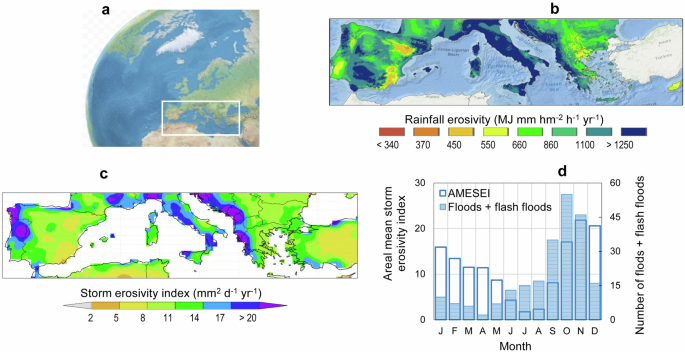
a Map of the Mediterranean region (white square, source: Shaded Relief, http://www.shadedrelief.com/natural2/globes.html); (b). Annual mean rainfall erosivity averaged over the period 2002−2012 (data sources: Climate Explorer, http://climexp.knmi.nl; GLDAS, 47); (c) Annual mean rainfall erosivity averaged over the period 2002−2012 (data source: Rainfall Erosivity Database on the European Scale REDES99). d Monthly AMESEI (empty histogram, 1970–1916), and sum of floods and flash-floods (blue histogram, 1940−2015) for the Mediterranean region (data source100).
This complexity gives rise to geographical and temporal variability in the distribution of rain-generating erosivity episodes. Synoptic circulation patterns play a pivotal role in shaping the annual and seasonal distribution of precipitation in the Mediterranean. These patterns advect a mixture of air masses from different regions, including the Atlantic, polar maritime and subtropical regions, and give rise to different degrees of rainfall erosivity (Fig. 2b). The AMESEI pattern (Fig. 2c) exerts its influence on three main areas of the Mediterranean region: the western part of the Iberian Peninsula, Italy, and the Balkans and western Greece. Notably, seasonal variability is pronounced (Fig. 2d), with 34% of storm erosivity occurring between September and November, coinciding with a stronger correlation with hydrological extremes. This period is particularly conducive to surface water floods and flash-flood events, which are more prevalent during this period (Fig. 2d, right axis).
The primary objective of the modelling technique employed in this study is to minimise uncertainty in the interannual variability by considering both large-scale influences, such as the El Niño-Southern Oscillation (ENSO) teleconnection, and smaller-scale climatic forcing represented by the variation coefficient of extreme rainfall. Designed for the Mediterranean region, the PARMAX(TVAR)-CSD model was trained using data from 1884 to 1992, and validated over the period 1993–2022. The PARMAX(TVAR)-CSD workflow, including the steps leading to its application to project climate conditions for the period 2023–2060, is illustrated in Fig. 3.
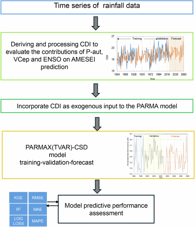
The workflow shows how the model was used to predict AMESEI in the Mediterranean region.
Results and discussion
Incorporating exogenous climate variables in decadal prediction models
Studies have demonstrated the efficacy of integrating decadal predictions into DDSMs due to the additional predictability provided by long-term climate oscillation signals45. This is supported by previous studies46, in which it was found that forecasts incorporating teleconnection patterns exhibited improved predictive ability for several years ahead compared to those without forcing46. These studies, including the present one, highlight the combined influence of internal climatic variability and external forcing (e.g., precipitation amount, variability of extreme hydrological events and ENSO) on decadal projections. Figure 4a illustrates the relationship between the AMESEI and two key precipitation metrics: the variation coefficient of extreme precipitation (VCep) and autumn precipitation amount (Paut). The VCep is a statistical measure that represents the relative variability of extreme precipitation events, calculated as the ratio of the standard deviation to the mean of extreme precipitation intensities over a given period. This metric highlights regions and timeframes where precipitation extremes exhibit relevant fluctuations, offering insights into the potential for erosive events. VCep is commonly used to quantify precipitation variability in climate studies (e.g.47). Throughout the Mediterranean region, VCep is positively correlated with AMESEI, with Pearson’s correlation coefficients (r) exceeding 0.5 in most areas and reaching values above 0.8 in some locations. These findings align with previous studies, such as48, which show that storm variability contributes to rainfall erosivity and sediment production. In contrast, Fig. 4b reveals a weaker relationship between autumn precipitation (Paut) and AMESEI, with correlation coefficients around 0.3, although values near 0.5 are observed in the Iberian Peninsula and Balkans. We acknowledge that Pearson’s correlations may miss complex, non-linear interactions. While future studies could explore mutual information to reveal deeper nuances in the data49,50, this study prioritised linear correlations to establish clear, quantifiable relationships for guiding model development. To further assess the combined influence of precipitation amount, variability of extreme hydrological events (as captured by VCep), and ENSO on decadal predictions, we used the Climate Driving Index (CDI) as exogenous data.
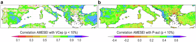
a Correlation between AMESEI and the variation coefficient of extreme precipitation (VCep) during the 1970−2016 period. Data sources: Global Land Data Assimilation System (GLDAS, 0.25° resolution. https://ldas.gsfc.nasa.gov/gldas; 47) and SDII-and Rx1day(s-aut). b Correlation between AMESEI and autumn precipitation amount (Paut) during the 1970−2016 period. Data source: E-OBS gridded dataset (0.25° resolution; https://www.ecad.eu/download/ensembles/download.php; Cornes et al. 76). Climate Explorer (http://climexp.knmi.nl) was used for map generation and updates.
The CDI serves as a key indicator of climate variability in the central Mediterranean region, incorporating both small–scale (autumn precipitation amount and variability of hydrological extremes) and large–scale (Niño3.4) climate-driven factors. Previous research on the Mediterranean region has shown that the variation coefficient of extreme precipitation (VCpe) and the storm erosivity index can be influenced by changes in short-term rainfall properties, shifts in seasonal distribution patterns of rainfall and year-to-year variability in precipitation51. Additionally, studies like52 have found El Niño years tend to see increased heavy rainfall, particularly across the central Mediterranean. This finding aligns with the combined effects captured by the CDI.
Our model incorporates various factors through the exogenous input (X ∙ βL) defined in Eq. 3, where X = CDI. The CDI, Eq. 5 is a composite metric combining key climatic and hydrological variables – ENSO(3.4), autumn precipitation (Paut), and the variation coefficient of extreme precipitation (VCep)—as detailed in the Data and Methods section. This index encapsulates the combined influence of these drivers on AMESEI, enhancing the model’s capacity to capture external forcing mechanisms. Figure 5a illustrates the linear relationship between the CDI, Eq. 5 and AMESEI. Notably, most data points reside within the 95% prediction boundaries, with only a few outliers (four points). This observation suggests a statistically significant relationship between AMESEI and the CDI, supported by a p-value < 0.001 in the ANOVA test. Additionally, the Durbin-Watson test53,54 was used to check for autocorrelation in the residuals. The Durbin-Watson statistic can range between 0 and 4, a value of 2.0 indicates no autocorrelation in the sample. Values from 0 to < 2 suggest positive autocorrelation, while values from 2–4 suggest negative autocorrelation. In our case, the Durbin-Watson statistic is 1.99 (p = 0.48), suggesting no evidence of serial autocorrelation in the residuals.
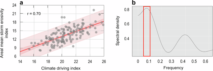
a Scatterplot of the relationship between the model’s exogenous input (Climate Driving Index) and AMESEI values from 1884 –2022. The inner (deep pink) and outer (light pink) areas indicate the 90% and 95% confidence intervals, respectively; (b) Spectral density plot of the distribution of frequencies in the Mediterranean AMESEI time-series The red box indicates the most likely frequency range for the PARMAX(TVAR)-CSD model cycle.
Furthermore, Pearson’s correlation coefficient of 0.70 indicates a moderately strong positive relationship between the variables. The mean absolute error (MAE) of 1.48, which is lower than the standard error of the estimates (1.94), further supports the accuracy of the estimates.
We evaluated the individual contributions of VCep, Paut, and ENSO indicators to the CDI by analysing their p-values. Among them, the autumn precipitation amount (Paut) has the highest p-value at 0.03. This justifies including all variables in the CDI equation. Next, the CDI time-series for the period 2023–2060 was processed and incorporated into the PARMAX(TVAR)-CSD framework (detailed in Supplementary Methods 2).
As a periodical model, the PARMAX(TVAR)-CSD framework incorporates a cycle parameter (m). Figure 5b illustrates the anticipated frequency spectrum for the fitted model parameters based on the AMESEI data (listed in Supplementary Data 1). The red boxes highlight the main cycles ranging from a frequency of 0.05 to 0.10. Based on this analysis, we set the cycle to approximately the peak frequency of 0.06, corresponding to a period m of about 41 years. This choice of a 41 year cycle is consistent with the peak frequency identified in the spectral analysis, and is further supported by the validation results, which show that this cycle improves the model’s predictive accuracy and aligns with observed patterns in the AMESEI data.
Decadal prediction skill and validation
The effectiveness of any prediction technique hinges on two key attributes: its accuracy and reliability. Determining this requires rigorous validation to avoid potential pitfalls like overfitting, where the model prioritises memorising specific data points over capturing broader patterns. In the context of DDSMs, one crucial step involves partitioning the data into training and validation sets. Striking the balance between these subsets is essential. Overweighting the training set can lead to overtraining, while an inadequate training set can hinder proper learning. The absence of established ratios for training, validation and prediction datasets26,55 presents a relevant challenge in optimising the validation of forecasting techniques. In general, the training dataset should account for a large portion, often >50% of the whole dataset56. In this work, the AMESEI dataset was divided into three subsets: training, validation and test. The proportions used were 62%, 17% and 21%, respectively. In our case, the test dataset corresponds to the prediction performed for AMESEI in years 2023- 2060.While there is no fixed rule for the lengths of these datasets, we allocated a 30 year period to the validation dataset to ensure it covered a conventional climate period. This left 109 years for training, which is ~62% of the total dataset. Although this extensive training period provides a robust foundation for the model, the potential for overfitting was carefully mitigated. First, as shown in Fig. 6a, the close agreement between the observed (blue) and modelled (orange) lines during the validation period indicates that the model accurately captures long-term trends without overfitting to training data. Then, the model’s performance was assessed using both training and validation subsets, and its error statistics (e.g., RMSE, MAE, MAPE) indicated consistently high accuracy and generalisability across these periods (Table 1), as further illustrated in Fig. 6b, c. For example, the MAPE for the validation period remained below 5%, well within acceptable thresholds57, with small error values (RMSE, MAE ≤ 0.15), and r and KGE values above 0.5, all indicating satisfactory performance.
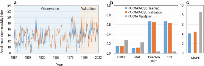
a Comparison of observed (blue line) and modelled (orange line) values, both showing a significant increasing trend (Mann-Kendal test: observed, p < 0.01; modelled, p = 0.02); (b, c). Performance indicators (RMSE, MAE, Pearson’s correlation coefficient, KGE and MAPE) for training and validation datasets, evaluated with (PARMAX-CSD) and without (PARMA) exogenous input.
We also compared the validation performance of the PARMAX(TVAR)-CSD model (which includes exogenous inputs) with a simpler PARMA(TVAR) model (which does not include exogenous inputs). As shown in Table 1, the PARMAX(TVAR)-CSD model was approximately twice as accurate as the PARMAX(TVAR), with lower RMSE, MAE and MAPE values. Its superior Pearson’s correlation coefficient (r) and Kling-Gupta Efficiency (KGE) confirm the benefits of using the longer training dataset alongside exogenous predictors. For the PARMAX(TVAR)-CSD model, Log Loss values of -1.52 (training) and -0.04 (validation) suggest a robust ability to generalise across both datasets, with minimal overfitting. In contrast, the significantly higher Log Loss value of 3.51 for the simpler PARMA(TVAR) model (validation) indicates a much greater uncertainty in its predictions. These results further highlight the advantage of including exogenous variables and the carefully designed dataset partitioning. While the results strongly support the robustness of the PARMAX(TVAR)-CSD model, caution is advised when extending forecasts to decadal scales due to inherent uncertainties.
Storm erosivity index decadal forecast
Understanding and forecasting the complexities of AMESEI dynamics requires navigating a variety of time scales, reflecting the intricate interplay of meteorological and climatic processes. These scales encompass both fleeting short-term changes and overarching long-term trends, posing relevant challenge for comprehending and managing the DHE framework. The last decade has witnessed the Mediterranean region endure numerous DHEs. Clusters of severe thunderstorms unleashed floods and flash floods across central Europe58. As Fig. 7 illustrates (blue line), the period between 2009 and 2012 saw storm power exceeding critical thresholds in the region. While accurately predicting the future impacts of climate change on the Mediterranean remains elusive, the increasing trend of storm damage is undeniable. This escalading damage highlights the influence of climate change on the severity and geographical distribution of meteorological phenomena linked to AMESEI.
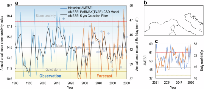
a Temporal evolution of observed (1997−2022, blue line) and forecasted (2023−2060, orange line) AMESEI values, with a 5 year Gaussian filter (dark line). Light blue dots represent the annual areal mean of daily rainfall at the 99th percentile (data source: CMIP5 ACCESS1-0 RCP4.5 dataset, Canadian Centre for Climate Modelling and Analysis; http://climexp.knmi.nl); (b) Smaller spatial-scale experiment with the PARMAX(TVAR)-CSD model; (c). Coevolution of AMESEI (orange line) and the annual areal mean of daily rainfall at the 99th percentile (blue line) showing the mean (bold horizontal grey line), and the 15th (yellow line, quiet storm) and 90th (orange line, storm erosivity exceedance) percentiles.
Building on the robust performance of our model, we have deliberately extended the forecasting horizon beyond the duration of the validation period, which spanned 30 years. Consequently, we extended the length of the forecasting period to 38 years. This extension allowed us to gain insights into potential climate conditions for the full decade 2050–2060. Figure 7 charts the projected annual AMESEI values (orange line) from 2023–2060. While an initial period of relative calm prevails, by 2040 extreme AMESEI values are projected to escalade markedly, exceeding the long-term median (horizontal grey line) by a noteworthy margin. The index then enters a phase of oscillation, fluctuating around the median and mirroring the smoothed trend depicted by the 5 year Gaussian filter erosivity index (dark line).
Following the projected surge in AMESEI by 2040, Fig. 7 indicates a shift in dynamics. The index is expected to stabilise around the long-term median (horizontal bold grey line), oscillating between the boundaries established by the quiet storm limit (bold ochre line). While peaks may still reach the storm erosivity exceedance threshold (bold red line), these events should become less frequent compared to the pre-2040 period. The 5 year Gaussian filter erosivity index (dark line) suggests a similar trend. Initially, it is predicted to decrease (dark line), reflecting the stabilisation of AMESEI. Around 2050, some years might even experience low storm erosivity levels (orange line), meaning a return to calmer conditions. However, these periods of reduced activity are unlikely to match the initial tranquillity observed before 2040. The quiet storm limit (15th percentile, bold ochre line) and storm erosivity exceedance threshold (90th percentile, bold red line) were assessed based on the historical distribution of AMESEI values from the baseline period (1997–2022). By defining thresholds associated with variability and extremes, these percentiles capture the lower and upper bounds of typical storm erosivity conditions and provide benchmarks to distinguish between relatively calm periods and extreme storm erosivity events.
The projected AMESEI values (Fig. 7a, orange line) exhibit consistently high interannual variability throughout the forecast period, mirroring the pattern observed in the historical data. While a statistically non-significant linear increase is detected based on the Mann-Kendall test (p > 0.05), further investigation is warranted to understand the underlying drivers of this trend.
Figure 7a reveals a compelling comparison between the projected changes in the 5 year Gaussian filter AMESEI (dark line) and the findings from the CMIP5 ACCESS1-0 historical r2i1p1 model output (blue light dots). Notably, the observed projections of the AMESEI filter closely resemble the annual mean of daily rainfall at the 99th percentile forecast under the RCP4.5 emission trajectories. This suggests a potential link between future AMESEI trends and extreme rainfall events as predicted by Global Circulation models (GCMs).
In particular, an interdecadal agreement is advisable for the projected changes over the whole period between two variables (Pearson’s correlation coefficient r = 0.41). On an interannual scale, however, the agreement between the two forecasts is less pronounced. This could indicate that the previous research on understanding extreme precipitation variability and its usefulness in supporting the decadal prediction of storm erosivity is incomplete.
It has also been shown that such variability, and to a lesser extent the annual ENSO signal, influence heavy precipitation in the Mediterranean. A trend toward greater driving of severe precipitation leading to rainfall erosivity has been observed since the early twentieth century59 and will likely continue in the future60,61. In this respect61, using a COSMO-Climate-limited area model (COSMO-CLM62) that takes into account the complex topography of Mediterranean areas, projected a climate signal for driving erosivity for maximum daily precipitation (Rx-1day), indicating an increase in some regions, particularly in northern Italy. More recently, using a large ensemble of Convection Permitting-Regional Climate Models under the RCP8.5 scenario63, identify a robust multi-model agreement for an increased frequency of heavy precipitation from central Italy to the northern Balkans, combined with a substantial extension of affected areas and an increase in intensity, area, volume and severity over the French Mediterranean, for the 21st mid-century. Most importantly64, confirmed that these events are likely to become more intense, more severe and more frequent, with the most dramatic changes expected in the central Mediterranean.
Moving from large to smaller spatial scales (Fig. 7b), it is striking to observe a significant agreement between these latest generation models and the outcomes of the PARMAX(TVAR)-CSD model run. In fact, looking at the projections for this area of the Mediterranean (Fig. 7c), the storm erosivity timeline between 2023 and 2060 increases (orange line), with a significant linear trend (Mann-Kendall trend test). Comparing the ACCESS1-0 model extreme CMIP5 projections (blue line) with the PARMAX(TVAR)-CSD projections (orange line), the latter shows a much stronger intensification of extreme AMESEI. In particular, the AMESEI increases linearly by 5 mm2 d-1 per decade. Furthermore, the AMESEI values are above the long-term mean (Fig. 7c, grey horizontal line) throughout the forecast period and also reach the 90th percentile around 2040 and before the end of the prediction period. This was also found in the results of 65, which indicate an increase in larger convective storms (mesoscale convective systems), which in turn can lead to larger damaging hydrological events with up to peak precipitation intensities across Europe. Furthermore, the AMESEI enhanced with a 10 year return period (statistically significant Mann-Kendal test, Fig. 8a, orange line) reflects a focus on intermediate extreme events that are more frequent and thus highly relevant for assessing storm erosivity trends over decadal timescales. This return period was selected because it balances the need for capturing impactful events without being skewed by rare outliers. Using a 10 year return period ensures that the projections remain robust and interpretable, especially when linking storm erosivity to other climate indicators, such as flood recurrence or extreme rainfall outcomes. Although higher return periods could represent rarer, more extreme events, these are less relevant to this study’s objective of understanding trends in moderately severe events that are likely to shape long-term erosion processes. This is consistent with the growth of areas affected by positive changes in flood recurrence of the CMIP5(E-HYPEcatch) ensemble mean (Fig. 8b, c), increases in extreme rainfall64, and their erosivity outcomes as predicted by more recent convection-permitting models27.
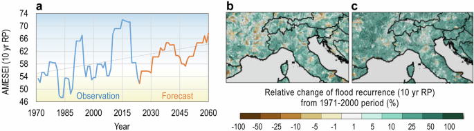
a Observed (blue line) and PARMAX(TVAR)-CSD forecasted (orange line) storm index; (b). Relative change in flood recurrence (%) from 1971−2000 period as forecasted for (b). 2011−2040 and (c). 2040−2071 with the CMIP5(E-HYPEcatch) ensemble mean (maps arranged using Climate Explorer; http://climexp.knmi.nl).
According to Panagos et al.17 and Uber et al.27, future climate change is projected to have a greater impact on rainfall intensity and erosivity, particularly in Europe. The influence of these hydrological drivers on soil erosion will be increased or decreased depending on the ability of land features, such as soil physical properties, land cover and land use, to buffer their effects under future climatic conditions66.
Disadvantages and limitations in decadal predictions
The current research shows that computationally efficient, data-driven statistical models can overcome many of the limitations of dynamical models. Our model does not explicitly account for the effects of atmospheric forcing (e.g. CO2 and aerosol concentrations), but their effects are likely to be implicitly included through the trend components of various variables. Extrapolation of trends may be appropriate when predicting lead times within a decade1. However, a comparison with the current convective-permitting dynamical models suggests that they may also be applicable beyond this timeframe.
The scarcity and inhomogeneity of observational data also make it difficult to assess how heavy precipitation varies with climate, even when precipitation observations are aggregated over large areas. Reanalysis data can overcome this issue. In any case, because of the inherent complexity of most real-world variables, it is virtually impossible to predict their future values routinely67. Forecast evaluation thus requires a thorough review of potential pitfalls and inaccuracies. Even if a model is well-designed with low bias and variance, the presence of interdependencies between temporally close values can lead to an increase in prediction errors over the forecast horizon67.
In addition, external climatic factors can cause discrepancies in the model and contribute to new sources of inaccuracy. The anticipated strengthening of the hydrological cycle, resulting in more precipitable water due to the Clausius–Clapeyron relation68, leads to an increase in sub-daily extreme convective precipitation69, which complicates forecast accuracy. In particular, extreme rainfall events are strongly influenced by dynamical factors involving feedback from latent heat exchange70. These factors are model-dependent and can increase model uncertainty in extreme precipitation responses33. It is thus crucial to recognise and overcome these challenges to ensure model robustness and reliability. Future research should prioritise the refinement of data-driven models, while comparing various types of models.
Conclusions
This study highlights the significance of advanced statistical technologies, such as time-varying autoregressive modelling with input climatic information, in enhancing our understanding and prediction capabilities of extreme weather events, specifically in the Mediterranean region. Despite challenges in generating sub-daily rainfall data, our findings underscore the value of these methodologies in addressing the complexities of hydrological extreme time series. While our research demonstrates progress in decadal prediction, it also emphasises the need for uncertainty-aware design paradigms to account for the complexities of predicting future storm-power and hydrological events. Integrating predictive information from dynamical models and statistical approaches could offer promising avenues for enhancing prediction skills and addressing long-term uncertainties71,72. By elucidating the implications of extreme weather events on various sectors, including human health and ecosystems, our study underscores the urgent need for improved prediction and understanding to mitigate their adverse effects on society and the environment. Our findings contribute valuable insights to the broader discussion on climate change adaptation and resilience strategies, particularly in regions vulnerable to extreme weather events like the Mediterranean. Continued research efforts in this field are essential for refining prediction models, developing robust adaptation strategies, and fostering resilience in the face of ongoing climate challenges, ultimately contributing to global efforts to address the impacts of extreme weather events.
Data and Methods
We compiled a consistent dataset spanning 1884-2022, incorporating multiple sources to ensure comprehensive coverage and reliability. Key variables include:
-
Simple Daily Intensity Index (SDII) and Daily Maximum Rainfall in summer-autumn (Rx1day-sa): Extracted from NOAA/CIRES/DOE 20th Century Reanalysis V3 dataset73, which provides global atmospheric and surface conditions reconstructed from historical observations;
-
Autumn precipitation (Paut): Derived from the GPCC v2020 dataset74, known for its high-resolution gridded precipitation analysis using station-based data;
-
ENSO (Niño3.4): Taken from ERSST v5 dataset75, offering global sea-surface temperature reconstructions critical for climate variability analysis;
-
Correlation map data: Sourced from GLDAS47,76, which provides a global dataset integrating observation-based meteorological data with model simulations.
For the AMESEI assessment, we opted to rely on reanalysis datasets due to the absence of long-term, high-quality daily precipitation records with complete geographic coverage across Europe. This limitation, highlighted by77, contributes to ongoing uncertainties in understanding variability in daily heavy precipitation intensities. The selected datasets provide a robust foundation for capturing spatial and temporal trends essential to our analysis.
Predictions were generated using the Time Series Lab78, Score Edition software V. 1.5 (https://timeserieslab.com), supported by Visual Recurrence Analysis (https://visual-recurrence-analysis.software.informer.com/4.9), and STATGRAPHICS (http://www.statpoint.net). SELFIS self-similarity analysis software (http://alumni.cs.ucr.edu/~tkarag/Selfis/Selfis.html) and CurveExpert Professional 1.6 (https://www.curveexpert.net) were also used for further statistical and graphical analysis. Model performance was assessed using several criteria, including root mean square error (RMSE), mean absolute error (MAE), mean absolute percentage error (MAPE), Pearson’s correlation coefficient (r), and Kling-Gupta efficiency (KGE). Lower values of RMSE, MAE, and MAPE indicate better model performance, with 0 being optimal and infinity representing the worst case. Pearson’s correlation coefficient (r) ranges from -1 to +1, with +1 indicating perfect correlation. The Kling-Gupta Efficiency (KGR), which ranges from -∞ to 1 (with 1 being optimal), was used79 to address the limitations of the commonly used Nash-Sutcliffe efficiency index by ref. 80. It is defined as: ({{{rm{KGE}}}}=1-sqrt{{(r-1)}^{2}+{left(alpha -1right)}^{2}+{left(beta -1right)}^{2}}). In this equation, r is the linear correlation between observations and simulations, α = σs/σo is a measure of the variability of the prediction errors, and β = µs/µo is a bias term, where µ and σ are the mean and standard deviation of the observations (sub-script O) and simulations (sub-script S). A KGE value >-0.41 is considered to indicate reasonable model performance. In addition, logarithmic loss (Log Loss) serves as an uncertainty metric, with lower values indicating better model performance and positive infinity representing the worst-case scenario (with no universally accepted thresholds for acceptable values).
Areal mean storm erosivity index assessment
The erosive power of a storm is accounted for by the rainfall erosivity factor (R-factor), which combines the effects of rainfall duration, intensity, and magnitude. To project the effectiveness of damaging hydrological events, it may be advisable to use a simplified form of rainfall erosivity timeframes81. Following the RUSLE (Revised Universal Soil Loss Equation) R-factor, which multiplies the kinetic energy of the rainfall (E) by its maximum 30 min intensity (I30)82, we define the Areal Mean Storm Erosivity Index (AMESEI) as the product of rainfall intensity and the highest daily rainfall. In this study, precipitation extremes are defined based on the highest daily rainfall (Rx1day) observed in the summer-autumn period, as this is a key indicator of storm erosivity in the Mediterranean region. Rather than focusing on entire storm events, we use the maximum rainfall intensity over a 24 hour period to quantify precipitation extremes.
The AMESEI (mm2 d-1) is calculated by multiplying the annual simple daily intensity index (SDII), which represents the mean intensity of daily precipitation events over the year, with the highest daily rainfall (Rx1day) in the summer-autumn period, as given in the equation:
Here SDII is the annual simple daily intensity index (mm d-1), and Rx1day(s-aut) is the highest daily rainfall in summer-autumn (mm d-1). Based on the equation of83, Rx1day(s-aut) expresses the maximum power of landscape disturbance since it covers a high ratio of hourly rainfall maxima for the Mediterranean region. While this approach does not explicitly consider characteristics such as event duration, multiple peaks, or time separation between events (which could be explored in future work), the high correlation between Rx1day(s-aut) and extreme rainfall in the Mediterranean supports its use as a reliable proxy for storm erosivity.
Exploratory AMESEI-data analysis and predictability
Exploratory data analysis (EDA) is an agile data analysis technique that focuses on graphical representation of data rather than statistical processing. The current framework includes a collection of data showing AMESEI at various timescales, emphasising its evolutionary aspects such as periodicity and autocorrelations. This can be used as a template to introduce the information for the selection criteria of the initial model. The process of exploring the data starts with basic data plots that evaluate patterns of fluctuation, changes in mean and variance, and the presence of any heteroskedasticity necessary to establish stationary conditions.
Figure 9a shows the annual evolution of AMESEI. The Mann-Kendall test, represented by the grey dashed linear trend, indicates a significant upward trend (p < 0.01). The log-transformed AMESEI data are shown in Fig. 9b (purple line), together with its variance evolution (Fig. 9c, green line), which reveals an oscillating trend, but without a significant (Mann-Kendall test, p > 0.05) long-term linear trend. In Fig. 9c, the variance of log-transformed AMESEI data is calculated using an 11 year moving window. The choice of an 11 year window aligns with common practices in climate and hydrological studies, where decadal-scale patterns are often analyzed to capture natural variability while smoothing out shorter-term fluctuations. This approach strikes a balance between retaining sufficient temporal resolution and reducing noise, enabling clearer identification of longer-term trends or oscillations. The 11-year period is particularly useful in regions like the Mediterranean, where interannual variability driven by climatic phenomena, such as ENSO, may influence storm erosivity. Future studies could explore different time window lengths to assess the sensitivity of variance trends to the chosen period.
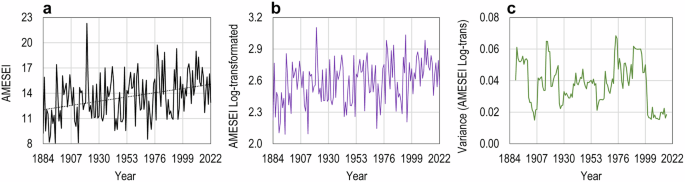
a Annual AMESEI time series (black line), with long-term linear trend (dashed grey line); (b). Log-transformed AMESEI data (purple line); (c). Variance estimates of log-transformed AMESEI data calculated using an 11 year moving window.
Exploratory data analysis includes autocorrelation function (ACF) and partial autocorrelation function (PACF), which can be used to analyse the correlation of data in time-series. Figure 10a shows the ACF, which connects log-transformed AMESEI data for various lags over residual values. The time-lag (k) shows the correlation between the log-transformed AMESEI data at time t and time t + k, which helps to define the order of the autoregressive model required for best data fitting. As the ACF and PACF generated on the standardised residuals of the original AMESEI time series were uncorrelated, we preferred to work on log-transformed data. It has been observed that log transformation leads to a stabilisation of the variance over time and facilitates the assumption of normality84. Instead, Fig. 10b shows the PACF, which correlates the log-transformed AMESEI data at different lags, but regresses the time-series values at all shorter lags. In this way, the ACF (Fig. 10a) shows a statistically significant positive correlation at lags 2, 3 and 5, with an abrupt transition to negative correlation, successively. The PACF (Fig. 10b) follows the same pattern, although the time series results are not significantly correlated. According to85, the model is an ARMA(P,Q), since the shapes of ACF and PACF follow a similar trend.
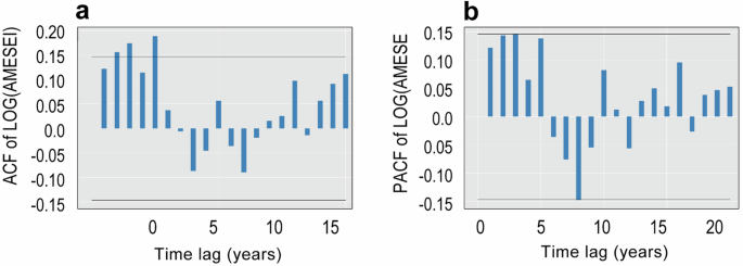
a Autocorrelation function (ACF) of log-transformed data, and (b). Partial autocorrelation function (PACF) on log-transformed data. Horizontal black lines indicate the 95% confidence limits.
The choice to use an autoregressive model of order AR(2) in Eq. 2 was based on the results presented in Fig. 10. Specifically, the ACF (Fig. 10a) showed significant positive correlations at lags 2, 3, and 5, with an abrupt transition to negative correlation afterward. Similarly, the PACF (Fig. 10b) showed a similar trend, with significant correlations at lags 1 and 2, and no significant correlations at higher lags. These results suggest that the AMESEI time series exhibits a significant dependency on its past values at lags 1 and 2, justifying the selection of AR(2) as the appropriate model order. This choice ensures that the model captures the temporal dependencies effectively, without overfitting to higher-order correlations that are not present in the data.
The choice to use the log-transformation proved to be the most appropriate option, as it improved the model performance during both the training and validation phases. The AMESEI residual distribution (not shown) was examined using the McLeod-Li (LM) test86. The test results showed that LM has a p-value of 0.87, well above the critical threshold of 0.05, indicating that the time series is not-heteroskedastic. Consequently, the preferred model was revised to PARMAX(2,0)m-CSD, where m = 41 represents the cycle associated with the location component. The value of m was determined through spectral density analysis, which identifies dominant periodicities in the data by analysing the frequency spectrum of the time series. This approach highlighted a relevant cycle corresponding to a period of ~41 years, which aligns with known decadal to multi-decadal long-term climatic oscillations linked to ocean-atmosphere interactions that influence the Mediterranean region87,88,89. The validity of m = 41 was further verified during the validation stage, where its inclusion improved predictive accuracy and supported other model parameters. This systematic assessment ensures that the chosen cycle is both statistically justified and climatologically meaningful.
Finally, predictability was explored in detail using the Hurst (H) exponent, which measures the long-term memory of time series data90. In other words, this statistic is crucial for characterising the memory and structural ramification of the time series. In a time series, the exponent defines the rate of stochastic processes, where 0 < H < 1. The exponent is closely related to the fractal dimension (D) of the time series through the relationship D = 2–H. This relationship indicates the autocorrelation or long-term memory characteristics of the time series. A time series with long-term oscillations between high and low values in adjacent pairs is represented by a value <0.5. This suggests a tendency to oscillate across a power-law function, and between high and low values over time. Short-term memory is represented by H = 0.5, where (absolute) autocorrelations fall rapidly to zero. A time series with long-term positive memory is indicated by a value of H > 0.5, which means that the autocorrelation decreases more slowly than exponentially and according to a power law.
To assess the presence of long-term memory in the AMESEI time series and its potential for forecasting, we employed the Rescaled Range (R/S) analysis, a non-parametric method for estimating the exponent H91. The original AMESEI data yielded an H of 0.63, indicative of strong persistence, suggesting that past trends are likely to continue. This supports the potential for reliable forecasting. To investigate the impact of detrending, we recalculated H on the detrended, log-transformed data. The resulting H of 0.51, while still suggesting weak persistence, may be an underestimate due to detrending’s potential to distort the true memory properties of the time series by removing trend while leaving other statistical properties unchanged (e.g. 92).
Model development
Parameterisation of the PARMAX(TVAR)-CSD model
Models can combine the efforts of multiple research teams to produce useful practical results that efficiently build knowledge93. In particular, given how these effects evolve over time, predictive models can reflect the influence of modest steps across multiple domains93. The main advantages of using the PARMAX(TVAR)-CSD model emerge when dealing with the largest amounts of information exchanged between states at time t–1 and time t, with the help of exogenous input climatic forcing, for decadal time in advance.
The random variable y at time t (yt) is represented as depending on both ({y}_{t-i}) and a fixed period m in the initial phase. A unique strategy for adding the periodic (m) component in the autoregressive model uses an additive structure consisting of two components.
The first is considered to be the location component94:
where yt is the AMESEI time series to be projected at time t over the year with period m; St is the random component, characterized as an AR (autoregressive) process with a mt (deterministic) periodic cycle of time m. The relevant parameters for the location component are outlined below:
where μ(L) is the model averaging; AR(2) is the autoregressive component of order 2. This suggests that the model depends on its past values ({y}_{t-i}), where i = 1 or 2. X is the exogenous variable, while βL is the corresponding parameter. The final score factor is the score vector of the (predictive) density of the observed time series, which is determined by the ability of score-driven models to deviate from the normal distribution.
The score-driven model has three main advantages78: (i) the filtered estimates of the time-varying parameter are optimal in a Kullback-Leibler, that is, an appropriate filtering mechanism over the genuine data generation process; (ii) because the models are observation-driven, their probability has been identified in closed form; and (iii) these models have comparable predictive performance to their parameter-driven competitors95.
The parameter equation of the second log-scale component is as follows:
σ denotes the standard deviation. βS is the corresponding parameter. As the time series is not heteroskedastic, the log-scale component, Eq. (4), has no autoregressive (AR) factor. In Eqs. (3) and (4), LevelL and LevelS represent the baseline or constant components for the location and scale (log-scale) components of the model, respectively. LevelL in Eq. (3) captures the overall mean or trend in the location component of the autoregressive model. It is a constant that adjusts the model to fit the baseline level of the time series before considering the autoregressive and periodic components. LevelS in Eq. (4) acts as the baseline level for the log-scale component, which is primarily used for modelling the variance or volatility in the data. It ensures that the logarithmic transformation of the variance has a meaningful baseline around which fluctuations can occur. These terms are essential for setting the baseline levels of the two components and ensuring that the model can account for both the trend (location) and the fluctuations (scale) in the time series data96 and40 provide further insights and numerical solutions to Eq. (2), (3) and (4).
Model design with exogenous climatic input
We employed an exogenous climatic input to establish and predict AMESEI for the coming decades, using the PARMAX(TVAR)-CSD model. This model was chosen for its ability to represent some of the internal natural variability involved in AMESEI, while also responding to climatic constraints. A Climate Driving Index (CDI) was used to enhance the data model. The inclusion of CDI features in the PARMAX(TVAR)-CSD model helps to accurately capture the behaviour of an autoregressive time series. The CDI is a composite index that incorporates multiple climatic variables known to influence storm erosivity. In particular, the variable X in Eq. (5) must include the CDI, which is a combination of the El Niño Southern Oscillation (ENSO(3.4)), autumn precipitation (Paut, mm d-1) and the variation coefficient of extreme precipitation (VCep). The CDI is then defined as a function of these variables according to the following expression:
where SD and M represent the standard deviation and mean, respectively, calculated over extreme rainfall (SDIIann and Rx1dsumm-aut) in mm d-1. The form of this equation was developed based on an integration of known climate drivers and their relationship to storm erosivity. The rationale for the combination of these specific variables lies in their established roles in influencing precipitation patterns and storm intensity. Specifically, ENSO is known to affect seasonal rainfall patterns and variability, which can influence the frequency and intensity of extreme weather events97. Autumn precipitation (Paut) has been identified as a key factor in determining regional hydrological conditions98. The inclusion of the variation coefficient of extreme precipitation (VCep) captures the variability of extreme rainfall events, further enhancing the predictive power of the CDI. The equation was derived through a combination of empirical relationships observed in the Mediterranean region’s climate data and the need to create a comprehensive index that could effectively capture the climatic drivers influencing AMESEI. The CDI shows a stronger relationship with AMESEI than when the INDIVIDUAL variables (ENSO, Paut and VCep) are considered separately, making it a more robust predictor for future storm erosivity patterns.


Responses