Climate warming and influenza dynamics: the modulating effects of seasonal temperature increases on epidemic patterns

Introduction
As global warming intensifies, human society is confronted with a series of profound environmental changes, among which the impact of climate change on public health has become increasingly significant. Climate change substantially influences the transmission of infectious diseases1,2,3,4. Concurrently, advancements in technology and accelerated urbanization have dramatically increased global population density and mobility. These factors interact with climate variables, further amplifying and complicating the transmission dynamics of infectious diseases5. Although diseases such as smallpox and cholera have been eradicated or effectively controlled6,7, the frequent emergence of new infectious diseases has raised global concerns8,9,10,11,12, particularly regarding respiratory infectious diseases such as Severe Acute Respiratory Syndrome (SARS)13, Middle East Respiratory Syndrome14, and Coronavirus Disease (COVID-19)15. The global pandemics caused by these pathogens not only challenge modern public health systems but also underscore the potential role of climate change in facilitating the spread of infectious diseases. Previous studies indicate that meteorological conditions such as temperature16,17, humidity18,19,20, and precipitation21,22 are critical determinants in the transmission and outbreak of influenza. Global warming-related extreme weather events are escalating in frequency, potentially intensifying the spread and incidence of infectious diseases23. While temperature interacts synergistically with other meteorological factors to influence outbreaks of respiratory infectious diseases, research has seldom concentrated on the primary trend represented by rising temperatures–the key indicator of warming. This oversight may lead to the neglect or misinterpretation of the independent or interactive effects of various meteorological factors under climate change. Consequently, this study aims to isolate temperature increases as an independent variable to explore its potential effects on influenza outbreaks, an area where understanding remains limited. Therefore, it is both important and urgent to investigate the impact of meteorological conditions on the occurrence and progression of influenza.
Influenza, an acute respiratory infectious disease caused by the influenza virus, is characterized by a complex and variable transmission mechanism. The Influenza A virus (IAV) and Influenza B virus (IBV) have received considerable attention due to their widespread prevalence and seasonal epidemic patterns24. Notably, the phenomena of antigenic drift24 and antigenic shift25 in IAV significantly enhances its transmissibility, thereby increasing the risk of influenza pandemics26. Historical pandemics, such as the 1918 Spanish Flu (H1N1)27,28 and the 2009 H1N1 influenza pandemic29, were initiated by mutated strains of IAV. Influenza viruses are primarily transmitted through respiratory droplets30 and exhibit distinct seasonal and regional transmission patterns31, particularly during winter months and in densely populated urban areas32,33,34. There is no consensus on the effect of temperature on influenza activity. Some studies have suggested that cold temperatures significantly increase the risk of influenza35,36,37, while some studies have shown that high temperatures are associated with influenza activity21,38, while others have found that both cold and high temperatures may affect influenza transmission39. The possible reason is that temperature has a specific effect on the transmissibility of influenza subtypes40. A study based on the distributed lag nonlinear model (DLNM) found that low temperature increased the risk of IAV and IBV in northern China, while low temperature and high temperature increased the risk of IAV in central and southern China, and the risk of IBV was only related to low temperature31. That’s the same conclusion as a study in Hong Kong41. In addition, the warming of the Earth in winter in the context of a warming climate will reduce the risk of future influenza epidemics32,42. However, rapid changes in weather32, especially temperature variability43,44, can affect the seasonality of influenza45 and increase the risk of influenza epidemics.
This study is dedicated to a thorough examination of how meteorological conditions, within the context of global warming, impact the occurrence and progression of influenza, utilizing models of infectious disease dynamics. We aim to uncover the mechanisms by which climate change influences influenza epidemics by dissecting transmission patterns and outbreak traits under various weather scenarios. We expect this research to lay a stronger theoretical groundwork for tackling potential influenza pandemics and to bolster the global public health system’s ability to effectively confront the challenges arising from climate change.
Here, we use the SIRS model to modify the transmission rate (beta) to the cosine transform including the time change, and set the temperature rise of 2.5 °C, 5 °C, 7.5 °C, and 10 °C. It was used to simulate changes in the number of influenza infections in a city of 500,000 people in the middle and high latitudes under warmer winters and warmer summers (see Methods more details). Table 1 presents the twelve research scenarios utilized in the idealized experiment, along with their corresponding interpretations.
Results
Simulation of influenza with and without seasonal variations
In a hypothetical urban setting with a population of 500,000, the initial outbreak of influenza, devoid of seasonal characteristics (Fig. 1A), resulted in a swift escalation of infections, reaching approximately 38,016 individuals. Analyzing the data on an annual basis reveals that influenza continued to recurrently infect urban residents following the conclusion of the initial large-scale epidemic, with the incidence of infections gradually declining. By the sixth year and beyond, infections leveled off at about 1693 individuals annually, deviating from the seasonal patterns commonly seen with influenza in real-world settings. When seasonal variations were factored in (Fig. 1B), the initial outbreak spiked to 34,282 infections. For the first six years, the infection pattern was similar to that in Fig. 1A; however, post-sixth year, the number of cases began to exhibit regular seasonal fluctuations, ranging from 745 to 3419 individuals. This aligns with the observed characteristics of influenza in mid-to-high latitude regions, peaking in winter and declining in spring and summer. This simulation effectively captures the progression of a new respiratory disease, evolving from a major outbreak to a seasonal pattern of infections that coexist with human populations.

The red inverted triangle indicates that (A) the number of infections is relatively stable, and (B) the number of influenza infections enters a seasonal cycle. The simulation parameters are set as follows: (L=4) years, (D=0.017) years, ({R}_{0}=5), (N=500,000) individuals, (left(Aright)beta =294) per year, (left(Bright){beta }_{0}=294) per year, ({beta }_{1}=0.04).
Influenza simulation under warm winter or high temperature in summer
Variations in the progression of influenza epidemics are observed under distinct warming scenarios. Given the unstable outbreaks of influenza observed during the initial phase of the model simulation, a warming signal was introduced following the stabilization of the epidemic in the tenth year. The simulation parameters were delineated as follows: (L=4) years, (D=0.017) years, ({R}_{0}=4), (N=500,000) individuals, ({beta }_{0}=235) per year, ({beta }_{1}=0.04). To elucidate the impact of rising temperatures, we calculated the difference in the number of infections before and after the temperature increase, defined as the number of infections post-temperature rise minus the number prior to the rise. This differential was subsequently presented using the tenth year as the baseline (i.e., year 0) to emphasize the effects of temperature fluctuations.
In the scenario labeled SW (Fig. 2A), a decline in the number of infections was observed during the autumn and winter seasons, followed by an upward trend in infections during the transition from winter to spring. In the subsequent autumn and winter, the number of infections increased in autumn but decreased in winter. When a continuous warming signal was introduced in the second winter (CW, Fig. 2B), the effects of warming in the first year mirrored those observed in SW. During the second autumn and winter, the number of infections that should have been increased in autumn decreased rapidly, with winter infections reaching their lowest point as temperatures continued to rise. Following the cessation of warming, the trend of decreasing infections in autumn and increasing infections in winter transitioned to a pattern of rising infections in autumn and falling infections in winter, with the increase in autumn infections surpassing the decrease in winter infections. Notably, there were no significant changes in infection rates during the spring and summer seasons. The severity of changes in the number of infections was positively correlated with temperature increases. In the SS scenario (Fig. 2C), the warming signal did not significantly alter influenza dynamics during the spring and summer months. Instead, a decrease in infections was noted in autumn following the end of the warming period, while winter infections increased. When the warming signal persisted through the second year’s spring and summer (CS, Fig. 2D), the number of infectious individuals continued to exhibit a decrease in autumn and an increase in winter, although the fluctuations in infection numbers were more pronounced. Again, no significant changes in infections were observed during spring and summer. Consistently, higher temperatures were associated with more dramatic changes in infection rates. A notable shift in the pattern of infection numbers was observed across all four scenarios, occurring 4 to 5 years following the cessation of the warming signal.
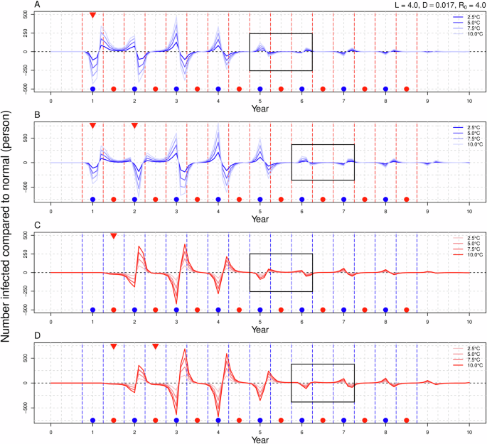
The horizontal axis represents time in years, with a value of 0 indicating the absence of warming signals, while the vertical axis represents the variation in the number of infections attributable to warming. A, B correspond to winter warming in either a single year or over two consecutive years, whereas (C, D) pertain to summer warming in similar timeframes. The red and blue dashed lines delineate the autumn-winter and spring-summer periods, while the gray dashed lines further segment the four seasons. Blue points signify the autumn-winter season, red points denote the spring-summer season, and red inverted triangles indicate the introduction of warming signals. The black rectangle highlights a shift in the pattern of the number of infected individuals.
In the scenario FW (Fig. 3A) and FS (Fig. 3B), persistent warming signals continued to disrupt the influenza epidemic, ultimately leading to the establishment of a new steady state (Fig. 3C). The ongoing warming during winter resulted in an increase in the number of infections during the autumn of the second and subsequent years, while the incidence of infections during winter decreased. Conversely, sustained warming during the summer was associated with a reduction in infections during the autumn of subsequent years, but an increase in winter infections. Figure 3C shows the annual changes in the total number of infections compared to the original sequence, with autumn and winter serving as the reference point for the commencement of the year. There was a slight increase in the number of infections during the first year of the winter warming, followed by a significant decrease in the second and third years, and a gradual increase in the fourth year. The changes in the number of infected individuals resulting from summer warming exhibited an opposite trend. Nevertheless, both scenarios ultimately converged to a steady state characterized by a slight decrease in the number of infections; notably, a greater rise in temperature corresponded to a more pronounced reduction in the number of infected individuals. The decrease in the number of infections attributable to winter warming was marginally greater than that associated with summer warming.

The horizontal axis represents time in years, with a value of 0 indicating the absence of warming signals, while the vertical axis represents the variation in the number of infections attributable to warming. A, B depict the comprehensive sequential warming effects of winter and summer, respectively. The red and blue dashed lines delineate the autumn-winter and spring-summer periods, while the gray dashed lines further segment the four seasons. Blue points signify the autumn-winter season, red points denote the spring-summer season, and red inverted triangles indicate the introduction of warming signals. C presents the changes in the cumulative number of infections for each year in comparison to the original sequence, with autumn and winter serving as the reference point for the commencement of the year.
Under the scenarios of SWS (Fig. 4A) and CWS (Fig. 4B), it is observed that if the temperature increase during winter is identical (either 7.5 °C or 10 °C), the variations in the number of infected individuals throughout the warming period remain consistent. Following the conclusion of the warming phase, the disparity in the number of infections across different scenarios is primarily attributed to the rise in summer temperatures. Specifically, a greater increase in summer temperatures correlates with a more significant rise or decline in the number of infections in both the current and subsequent years. When summer warming is held constant (either 2.5 °C or 5 °C), a greater increase in winter temperatures corresponds to more substantial fluctuations in the number of infections during that year and in the following years. Among the four scenarios involving winter and summer warming, the variation in infection numbers is greatest in the (10, 2.5) scenario and smallest in the (7.5, 5.0) scenario. In the context of the SSW (Fig. 4C) and CSW (Fig. 4D), it is noted that when the temperature rise in summer (or winter) is equivalent, a higher temperature increase in winter (or summer) results in greater fluctuations in the number of infections. However, we found that the strong trend of influenza development under the two different warming sequences was is fundamentally similar, with a shift in the pattern of increase and decrease; specifically, the number of infected individuals rises in autumn and declines in winter following the conclusion of the warming period. The results for the FWS (Fig. 5A) and FSW (Fig. 5B) are analogous to those of FW and FS scenarios and will not be elaborated upon here.

The horizontal axis represents time in years, with a value of 0 indicating the absence of warming signals, while the vertical axis represents the variation in the number of infections attributable to warming. A, B depict scenarios in which warming occurs in winter first, followed by warming in summer, either over a single year or over two consecutive years, while (C, D) illustrate scenarios where warming occurs in summer first, followed by warming in winter, again for either a single year or two consecutive years. The black dashed lines delineate the autumn-winter and spring-summer periods, while the gray dashed lines further segment the four seasons. Blue points signify the autumn-winter season, red points denote the spring-summer season, and red inverted triangles indicate the introduction of warming signals.

The horizontal axis represents time in years, with a value of 0 indicating the absence of warming signals, while the vertical axis represents the variation in the number of infections attributable to warming. A describes the scenario of the whole series warming first in winter and then in summer, while (B) illustrates the scenario of the whole series warming first in summer and then in winter. The black dashed lines delineate the autumn-winter and spring-summer periods, while the gray dashed lines further segment the four seasons. Blue points signify the autumn-winter season, red points denote the spring-summer season, and red inverted triangles indicate the introduction of warming signals.
The influence of different parameters on influenza simulation
In the context of the SIRS model, varying parameter settings revealed that the response of the infected population to increases in temperature exhibited sensitivity characteristics. A higher basic reproduction number (R0) was associated with a shorter oscillation period, allowing the number of infections to return to their original steady state more rapidly, thereby diminishing the impact of the warming signal (Fig. 6A, B). An analysis of the dynamic changes in the actual number of infected individuals (Fig. 7) indicated that a larger R0 corresponds to a lower peak prevalence of influenza, a higher trough, and an increased frequency of peaks occurring during the summer and autumn seasons. When the average immunity duration L is reduced, the oscillation period shortens, facilitating a quicker return to the original steady state (Fig. 6A, C). As L increases, the peak value of the actual number of infected individuals decreases, and the timing of the peak is slightly delayed. Furthermore, an increase in the average infection period (D) does not significantly alter the oscillation period (Fig. 6A, D); however, it results in a gentler rise and fall of the wave crest and trough. Concurrently, the amplitude of the actual number of infected individuals diminishes, the trough value increases, and the timing of the peak is also slightly postponed.

The horizontal axis represents time in years, with a value of 0 indicating the absence of warming signals, while the vertical axis represents the variation in the number of infections attributable to warming. The parameters used in (A) are: L = 4 years, D = 0.017 years, R0 = 4, N = 500,000 individuals, β0 = 235 per year, β1 = 0.04. All parameter changes are based on the above settings. B R0=15. C L = 8 years. D D = 0.027 years. The red dashed lines delineate the autumn-winter and spring-summer periods, while the gray dashed lines further segment the four seasons. Blue points signify the autumn-winter season, red points denote the spring-summer season, and red inverted triangles indicate the introduction of warming signals.

The horizontal axis represents time in years, with a value of 0 indicating the absence of warming signals, while the vertical axis represents the variation in the number of infections attributable to warming. The red inverted triangles denote the introduction of warming signals. N.C. parameter settings: (L=4) years, (D=0.017) years, ({R}_{0}=4), (N=500,000) individuals, ({beta}_{0}=235) per year, ({beta}_{1}=0.04). All parameter changes are based on the above settings.
Discussion
In this study, we employed the SIRS model to systematically simulate influenza virus outbreak patterns under various warming scenarios. The results demonstrated that different warming signals have different effects on influenza transmission. The addition of separate hot summer and warm winter signals caused large fluctuations in the number of influenza infections and gradually disappeared. In the case of long-term warm winter and high temperature in summer, the number of infected people showed a tendency to readjust to a new stable state, and the average annual number of infected people was lower than the level before warming. Different parameters also influence the effect of warming signals on influenza activity.
Empirical evidence indicates that influenza viruses exhibit prolonged survival at lower temperatures and relative humidity46,47, while cold and dryness also facilitate aerosol transmission of these viruses48. Furthermore, warm weather tends to encourage outdoor activities, and increased sunlight exposure is linked to enhanced vitamin D synthesis, which in turn bolsters immune responses49,50. Compared with IBV, the risk of IAV is more susceptible to the influence of vitamin D levels51. The increased duration of time spent outdoors impedes viral transmission. In addition to affecting virus survival time, transmission mechanisms, and the human immune system response, temperature also significantly affects the spread and risk of influenza virus infection by affecting population exposure patterns. In cold weather, individuals mainly congregated in poorly ventilated spaces, increasing the proximity and duration of proximity of individuals to others52,53, which elevates the risk of infection48,54. For students, the heat increases school contact53,55. Community contacts are the people most influenced by the weather, for every 1 °C increase in temperature, the number of people in contact is expected to decrease by 2.5%56.
In this study, we focused on the influence of temperature rise signals of varying intensity and duration on the occurrence and development of influenza by incorporating diverse warming signals into the SIRS model for simulation analysis. The impacts of warming are identified and categorized into three primary types: seasonal, interannual, and interdecadal effects. Taking winter warming as an example, the seasonal impact is observed to be the most direct and significant. During autumn and winter, the number of infections may increase or decrease considerably, while the warming signal exerts relatively minimal effect on the number of infections in the spring and summer due to weaker influenza virus activity. This seasonal change signifies that influenza exhibits heightened activity during the autumn and winter months. Consequently, the incidence of infections typically diminishes in the year characterized by warming, resulting in the accumulation of a substantial population of non-infected susceptible individuals. This accumulation predisposes the infection count to a significant upsurge in the autumn of the first year subsequent to the cessation of the warming signal. Over time, the interannual repercussions of the warming signal persist, continually propagating backward into subsequent years until the signal either attenuates or altogether ceases. As the signal disappeared, we observed changes in the pattern of increases and decreases in the number of infections. This phenomenon may be attributed to the total number of infections being slightly elevated in the years following the cessation of winter warming, suggesting that as the population of immune individuals accumulates over time, the number of infections decreases in accordance with epidemiological dynamics. In summer warming scenarios, as the number of susceptible individuals accumulates over time, the number of infected individuals is likely to rise. Consequently, this pattern shift is interpreted as an indication that the effects of warming signals have concluded. The influence of the warming signal on influenza prevalence diminished significantly by the eighth year, suggesting that the impact cycle of extreme climatic events on influenza may range between six to seven years. Upon the sustained warming of the entire sequence, despite the fluctuations in the number of infected individuals due to environmental changes, a new equilibrium state will ultimately emerge. Typically, the total number of infected individuals in this new state will be lower than the pre-warming level. This emergent homeostasis suggests that the influenza virus is adapting to the novel climatic conditions, thereby altering the transmission trajectory of the virus. This interdecadal variation underscores the potential long-term warming effects on influenza transmission patterns. In the context of global warming, seasonal, interannual and interdecadal variations collectively constitute a multifaceted landscape of influenza transmission, intricately interwoven and mutually reinforcing.
The selection of different parameters significantly influences the simulation of influenza dynamics. A high R0 value typically indicates rapid disease transmission57,58, leading to a swift increase in the number of infected individuals during an outbreak. This rapid spread can facilitate a quicker return to an equilibrium state of transmission. In the warming state, the observed reduction in the fluctuation of infection numbers may be attributed to an increase in R0, which markedly affects the spread speed, thus rendering the impact of warming on infection numbers relatively minimal. When the average immune time L is small, individuals sustain immunity for a limited time following infection, resulting in accelerated fluctuations in the proportion of susceptible and infected persons, and the transmission rate will quickly return to the new equilibrium state. In the case where (L=0), the model simplifies to an SI (Susceptible-Infected) model57, wherein the absence of immunity allows for continuous reinfection. Furthermore, an increase in the duration of the mean infectious period (D) extends the time from infection to the manifestation of symptoms, thereby prolonging the infectious cycle. This extension yields flatter and less volatile epidemic peaks and troughs, indicating a smoothing of virus spread. Consequently, while the peaks of influenza seasons may become less pronounced, the overall duration of the epidemic tends to increase.
We calculated the peak-to-trough ratio (PTR) of the simulation results regarding the number of infected individuals across the entire series of temperature rises (FW, FS, FWS, and FSW, Table 2). Our analysis revealed that a greater rise in temperature during winter yielded a smaller PTR, indicating a diminishing magnitude in the fluctuations of infection numbers. Previous research has highlighted that seasonal patterns of influenza in low-latitude regions exhibit ambiguity and relatively low volatility59. This study further confirmed that as winter temperatures rise, the epidemic volatility associated with influenza significantly diminishes. Consequently, rising winter temperatures are likely to align incidence patterns in middle and high latitude regions more closely with those observed in low-latitude areas, thereby reflecting the validity of our model to some extent. Conversely, the trend of PTR change during summer is contrary to that observed in winter. In scenarios where both winter and summer experience simultaneous temperature increases, results from FWS were largely consistent with FW outcomes; however, summer warming primarily influenced population change magnitude rather than overall trends. Notably, the results of FSW did not align with those of FS but exhibited greater similarity to those of FW. Based on the analysis of PTR, we believe that the impact of winter warming on influenza dynamics far surpasses that of summer warming. Therefore, future research should focus more on the potential implications of the warm winter phenomenon on the development of influenza epidemics.
In the SIRS model, we only focused on the impact of temperature changes on the occurrence and development of influenza. In fact, humidity is also one of the important factors affecting the influenza transmission35,60,61. Moreover, research has indicated that absolute humidity, rather than relative humidity, plays a key role in determining influenza morbidity during the flu season62. In fact, temperature and humidity do not have an effect on the spread of influenza alone, but a synergistic effect. In our previous study59, we found that the synergistic effect of temperature and specific humidity was more pronounced in temperate countries, but weaker in tropical countries. This synergy can be divided into two modes, cold-dry and warm-wet, and a certain threshold needs to be reached before the switch between mechanisms can occur. Aerosols not only exacerbate haze pollution63 but also serve as the primary carriers of respiratory disease pathogens30,64,65, significantly influencing the spread of influenza66,67. Among the factors affecting aerosol transmission, temperature and humidity play a crucial role in the transmission mode of influenza by regulating the survival and transmission efficiency of influenza virus in aerosols48. Research indicates that relative humidity (RH) has a significant effect on the infectivity of influenza virus in aerosols68,69. In low RH environment, the biological decay rate of influenza virus is lower, which prolongs its survival time in aerosol and enhances the transmission efficiency67. In addition, low temperatures (e.g., 5 °C) help enhance aerosol propagation, while high temperatures (e.g., 30 °C) block airborne transmission at all RH levels16. In addition to the above factors, other variables such as crowding61,70, the indoor and outdoor environment71, air pollution72, and population immunity levels73 also affect the seasonal outbreak and transmission of influenza to varying extent. Therefore, future research should consider introducing more factors into SIRS models to more accurately predict the seasonal patterns and transmission dynamics of influenza.
In conclusion, our study reveals new characteristics of influenza transmission patterns in the context of global climate change, highlighting the importance of winter temperature changes in the spread of influenza. It also suggests that traditional seasonal patterns associated with influenza may undergo transformation as a result of global warming. In order to effectively respond to possible future influenza outbreaks, there is an urgent need to develop more scientific and flexible surveillance and control measures to protect public health.
Methods
SIRS model
Dynamic models of infectious diseases are essential tools for understanding the transmission mechanisms of the influenza virus. The classical SIR (Susceptible-Infectious-Recovered) model divides the population into Susceptible (S), Infected (I), and Recovered (R)58,74,75. The time distribution of population types in different compartments can be calculated by ordinary differential equation. According to the different characteristics of disease, the Exposed (E) and Susceptible (S) are introduced respectively on the basis of the SIR model to form the SEIR (Susceptible-Exposed-Infectious-Recovered) model76,77 and the SIRS (Susceptible–Infected–Recovered–Susceptible) model78. These models can effectively simulate the transmission processes of infectious diseases within populations79,80,81, and reflect the dynamics of transmission under varying environmental conditions by adjusting model parameters, thereby providing valuable insights into the behavior of influenza outbreaks.
In this study, we utilize the SIRS model to analyze influenza dynamics. This model accounts for the gradual decay of human immunity to the influenza virus over time by incorporating a loss of immunity term (s) into the SIR framework. Consequently, individuals can regain susceptibility after progressing through the stages of susceptibility, infection, and recovery. The equations governing the SIRS model are as follows:
where t represents time in years, S denotes the susceptible population, I indicates the infected individuals, R refers to the recovered individuals (i.e., the number of immune individuals), and N signifies the total population. L represents the average duration of immunity, which refers to the average time that an individual’s immune protection persists following recovery from the illness. D denotes the mean infectious period, defined as the average time interval between an individual’s infection and the onset of disease symptoms. The basic reproductive number R0 is defined as the average number of secondary infections generated by a single case during its infectious period within a fully susceptible population. When ({R}_{0}, <, 1), the disease gradually disappears. When ({R}_{0}, >, 1), the disease persists and forms endemic diseases. The transmission rate is denoted as (beta), ({R}_{0}) equals Dβ. In this model, the intrinsic period of oscillation of the disease is (T=2pi sqrt{{DL}/({R}_{0}-1)}) 80.To account for the seasonal variation of influenza, the transmission rate (beta) is modified to include a cosine transform over time:
In this formulation, ({beta }_{0}) is the non-seasonal transmission coefficient, ({beta }_{1}) is the seasonal oscillation transmission coefficient, and ({R}_{0}=D{beta }_{0}). In this study, the average duration of immunity (L) for the influenza virus was established to be between 4 to 8 years, the mean infectious period (D) was set at 6 to 10 days, and the basic reproductive number (({R}_{0})) ranged from 4 to 1662,80,82,83. The seasonal oscillation transmission coefficient (({beta }_{1})) was determined to be 0.0480.
Experimental design
To enhance our understanding of the effects of rising temperatures on influenza outbreaks and the transmission rates of the virus, we designed an ideal experiment with an urban population of 500,000 individuals. This experiment was grounded in the SIRS model and was conducted in mid-to-high latitude regions, where influenza outbreaks predominantly occur during the winter months34,59. The temperature range for the study was established between −20 °C and 30 °C to accurately reflect real climatic conditions. In assessing the infection rate (beta left(tright)), the (cos left(2pi tright)) sequence, which has a value range of [−1, 1], was compared to the normalized temperature sequence, which is (-fleft(Tright)=cos left(2pi tright)). To explore various warming signals, we developed distinct sequences for warm winters and high summer temperatures. For the warm winter sequence,
The temperature increase was implemented throughout the entire autumn and winter period, with minimum temperatures raised by 2.5, 5, 7.5, and 10 °C, respectively. In the summer high-temperature sequence,
The increase in temperature occurred throughout the entirety of the spring and summer seasons, with the maximum temperature rising by 2.5, 5, 7.5, and 10 °C, respectively. Figure 8 illustrates the variation in the transmission rate sequence following the warming period.
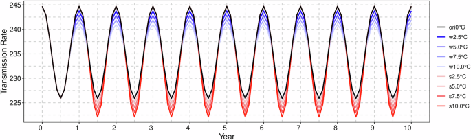
The black line denotes the original transmission rate, while the blue line reflects the alterations in infection rates subsequent to winter warming. Conversely, the red line indicates the changes in infection rates following summer warming. The numerical values in the legend correspond to the increments in temperature.
In this study, we explored scenarios where increased summer temperatures coincide with milder winters to enhance the experimental design’s realism. We hypothesized that the severity of winter warming would surpass summer warming, mirroring real-world climate change trends84,85,86. The specific warming combinations employed in the experiment were as follows: (7.5 °C, 2.5 °C), (7.5 °C, 5 °C), (10 °C, 2.5 °C), and (10 °C, 5 °C).
Responses