Compound coastal flooding in San Francisco Bay under climate change

The San Francisco Bay Area (SF Bay), the fifth largest metropolitan area in the United States, is important locally and globally due to its prosperous economy, diverse culture, and unique landscape^1,2,3. However, some low-lying areas of SF Bay experience coastal flooding^2,4 and the SF Bay Area is at risk of worsening compound coastal flooding due to multiple forcing factors such as tides, waves, and river discharge (RD)^5,6,7,8,9,10. As sea level rises due to climate change^11,12, increasingly frequent extreme sea-level events are projected to inundate low-lying areas around the Bay^{2,3,5,13,14,15} with potentially disastrous effects on public health, infrastructure, and ecosystems^{3,5,11,13,16,17}. In addition, warmer temperatures may increase the intensity of extreme rainfall^18,19 and runoff²⁰, resulting in higher RD and changes to flood risk¹⁸. Climate change may also result in more precipitation falling as rain instead of snow^11,18, leading to more direct runoff and causing higher peak RD in SF Bay¹⁸, even with some flood control capacity provided by reservoirs upstream in the Sacramento and San Joaquin river basins. Therefore, compound flood risk has the potential of significantly increasing as a result of both sea-level rise (SLR) and higher RD^{3,21,22,23,24,25}. It is critical to investigate the impact of climate change on compound coastal flooding for climate adaptation planning and efforts to increase coastal resilience^{26,27,28,29,30,31}.

The influence of climate change on compound coastal flooding in SF Bay remains underexplored. Most existing research focuses on coastal flooding under SLR^{2,5,17,32,33,34,35} while only a few studies have focused on compound flooding analysis under both SLR and higher RD due to climate change^36,37. Much of the existing research employs dynamical approaches^{2,17,32,33,34,36,38}, while a few studies use statistical approaches³⁵ or hybrid statistical-dynamical approaches³⁷. Dynamical approaches are capable of accurately simulating spatially varying water levels for flooding analysis by using high-fidelity hydrodynamic modeling techniques^39,40. However, heavy computational burden limits the applicability of this approach for investigating many forcing combinations and flood scenarios, especially for large and complex coastal areas such as SF Bay^40,41. Statistical approaches efficiently assess compound flooding by relying on techniques such as extreme value analysis for historical data analysis^35,42,43. Statistical approaches are, however, typically unable to perform flooding analysis for any location of interest or explore all possible forceing combinations due to limited spatially and/or temporally varying data^{44,45,46,47,48}, particularly when considering climate change^40,49,50. Like many hybrid statistical-dynamical approaches applied in other coastal areas^41,51,52,53, the hybrid approaches for compound flooding analysis in SF Bay under climate change³⁷ typically first use statistical techniques to efficiently sample forcing combinations for return level events under climate scenarios and then pass the forcing conditions into computationally expensive hydrodynamic models to simulate water levels. These types of hybrid approaches may not identify extreme compound flooding driven by different combinations of forcings that are not captured by statistical techniques^8,45. Alternative hybrid modeling approaches have been developed by merging statistical and numerical modeling to generate the response of dynamical approaches under a full range of possible forcing combinations^{40,45,54,55,56}.

This study uses the hybrid statistical-dynamical approach developed in ref. ⁵⁶ to analyze compound coastal flooding in SF Bay under a range of climate change scenarios. By combining a stochastic generator of compound flooding drivers, a high-fidelity hydrodynamic simulator, and machine learning-based surrogate models; the hybrid framework can investigate the full range of plausible forcing combinations for compound flooding analysis, applied to SF Bay. Here we consider six representative climate change scenarios and a baseline scenario without climate change for compound flooding analysis using the hybrid framework. The six climate change scenarios (see Table S1 for details) are defined by linking three SLR projections (low, medium, and high impact) with six combinations of future warming and thermodynamic scaling of daily precipitation. Each climate change scenario is used to generate 100 hourly synthetic simulations of 500 years each, allowing infrequent extreme return level events to be analyzed. The impact of climate change on compound coastal flooding is investigated in terms of flood magnitude, flood frequency, and the relative contributions of different drivers to extreme flooding. These three metrics can be used to inform climate change adaptation and coastal resilience planning in the SF Bay Area, and the hybrid statistical-dynamical approach demonstrated here can be generalized for compound coastal flooding analysis in other complex coastal areas under climate change.

Here we present hybrid model results revealing the potential impacts of climate change in SF Bay (Fig. 1) in terms of flood magnitude, frequency, and the relative contributions of forcings to flood events. All analyses are performed at 16 representative locations that are approximately evenly distributed along the centerline of the Bay (i.e., locations 3–18) while locations 1 and 2 near the Delta mouth are used as auxiliary points for analysis. The magnitude and frequency of possible flooding are illustrated at locations 3–18, and the relative contributions of drivers are focused on the 7 locations in the North Bay (i.e., locations 3–9) considering the modest impact of the climate change scenarios considered here on the spatial variability of the relative contributions elsewhere in the Bay.

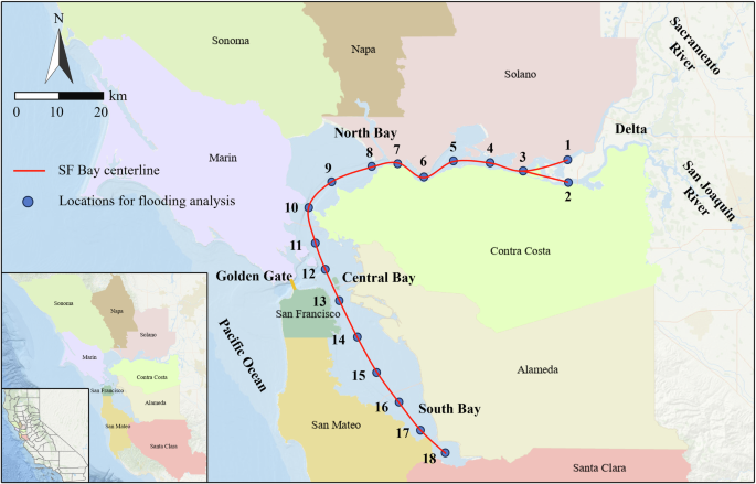
The X and Y coordinates of the 18 locations are provided in Table S2. The Bay is classified into the North Bay (locations 1–9), Central Bay (locations 10–14), and South Bay (locations 15–18) for convenience of analysis. Note that locations 1 and 2 are near the Sacramento San Joaquin Delta mouth where Sacramento and San Joaquin rivers flow into the Bay, and location 3 is where the two rivers converge in the Bay. Inset maps show the SF Bay Area surrounding (nine counties, i.e., Alameda, Contra Costa, Marin, Napa, San Mateo, Santa Clara, Solano, Sonoma, and San Francisco) and including SF Bay, and its location in CA.

Full size image

Flood magnitude

Stochastic 100-year return level total water level (TWL) event distributions under each of six climate change scenarios and a baseline scenario without climate change (Table S1) are computed across 100 hourly simulations of 500 years each. The flood magnitude distributions for each scenario are shown (Fig. 2a–c) for locations in SF North Bay (location 5), Central Bay (location 12), and South Bay (location 18, Fig. 1). Extreme TWLs show larger variability under more extreme climate change scenarios (i.e., higher temperature and larger thermodynamic scaling rate of extreme precipitation) in the North Bay. For example, extreme TWLs peak at a larger value, have a greater variation, and are characterized by having a more right-skewed distribution under the climate change scenario C6 at location 5 (Fig. 2a). The mean, standard deviation, and skewness of the 100-year return level TWLs under different climate scenarios are provided in Table S3. However, there is similar variability of extreme TWL events under all climate change scenarios in the Central and South Bay.

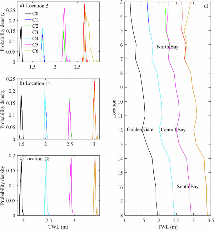
a–c Distributions of 100-year return level TWLs under different climate scenarios at locations 5, 12, and 18 (~26 km, 80 km, and 132 km seaward from the Delta, respectively). d Spatial distribution of mean extreme TWLs under different climate scenarios along the centerline of SF Bay. Different colors represent different climate scenarios, where C0 is a baseline scenario without climate change and C1 − C6 are six climate change scenarios with higher river discharge and SLR defined in Table S1. Note the lines overlap with each other under C1 and C4, or C2 and C5, or C3 and C6 at almost all locations in the Central and South Bay.

Full size image

The 100-year return level TWLs over the 100 simulations at each location are averaged to obtain the spatial distribution of the mean extreme TWLs (Fig. 2d). The spatial variability under different climate scenarios is similar in the Central and South Bay. However, spatial variability is projected to be smaller under more extreme climate change scenarios in the North Bay (i.e., C1 > C4 > C2 > C3 > C5 > C6).

In addition, the difference in variability between scenarios of climate change with the same temperature but different thermodynamic scaling rates of extreme precipitation is greater in scenarios of higher temperature, i.e., the largest difference of TWLs is 0.26 m, 0.10 m, and 0.02 m between C3 and C6, C2 and C5, and C1 and C4, respectively.

Flood frequency

The amount of time in which nuisance, minor, moderate, and major flood thresholds are exceeded^56,57,58 each year is counted for each climate scenario in the 100 simulations. Fig. 3a–d shows the distribution of the number of hours per year that water levels exceed these flood thresholds at a location in the North Bay (the distributions in the Central and South Bay are similar). As expected, the hours of threshold exceedances per year increase with the more extreme climate change scenarios. Overall, the hours of threshold exceedance per year demonstrate a smaller variability when some simulations result in no threshold exceedances and larger variability otherwise. However, climate change does not have a large impact on variability when all simulations have threshold exceedances.

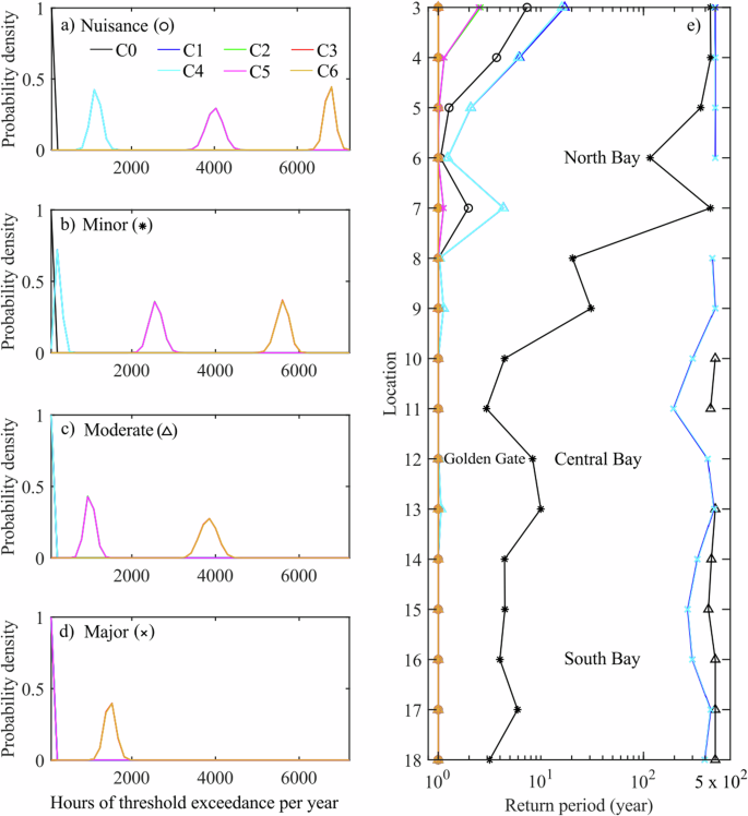
a–d Distributions of the number of hours per year in which nuisance, minor, moderate, and major flood thresholds are exceeded under different climate scenarios at location 5 (~26 km seaward of the Delta, Fig. 1). e Spatial distribution of nuisance (circle), minor (asterisk), moderate (triangle), and major (cross) flood frequencies under different climate scenarios along the centerline of SF Bay. Note the lines almost overlap with each other under C1 and C4, or C2 and C5, or C3 and C6 in (a–d). Moderate flood frequencies at some locations and major flood frequencies at all 16 locations under C0 are not plotted if no such flood events are found in analysis.

Full size image

The mean flood frequency in terms of return period is calculated by averaging over the 100 simulations for the four flood thresholds under each climate scenario at each location (Fig. 3e). The spatial variability of the four flood thresholds simulations are smaller under more extreme climate change scenarios. For example, nuisance and minor flood return periods (minor flooding in particular) decrease from North Bay to South Bay under C0. Flood events exceeding both are projected to occur more frequently than once per year at all locations under any considered climate change scenario. However, the return period of major flood threshold exceedance events demonstrates relatively large spatial variations under C1 and C4 (i.e., both 195.8–500 years), small variability under C2 and C5 (i.e., 1–2.6 years and 1–2.5 years), and no variability under C3 and C6 (i.e., occurs more than once per year).

Relative contributions of flood drivers

The relative contribution, and associated variability, of each non-SLR forcing to the five most extreme events in each simulated hourly 500-year time series under different climate change scenarios is investigated (Fig. 4a–f for location 5) (the relative contribution of SLR is straightforward and provided in Fig. S1). The top five events in each time series represent TWL events with 1% or less chance of occurring in any given year. Overall, tidal levels associated with extreme TWLs (Fig. 4a) share a similar range and variability under all climate scenarios. The water levels (WLs, i.e., the water levels due to any combination of drivers) due to non-tidal and non-SLR drivers other than RD (i.e., MMSL, waves, SLP, and winds in Fig. 4b–e) also have a similar order of magnitude under all climate scenarios. However, these WLs overall shift from a more left-skewed distribution to a less left-skewed distribution under more extreme climate change scenarios, e.g., the skewness of the WLs due to MMSL is -1.52 and -0.11 under C1 and C6, respectively. The WLs associated with these non-tidal and non-SLR drivers become approximately zero under scenario C6. Unlike other non-tidal and non-SLR drivers, the WLs due to RD (Fig. 4f) have a larger range (e.g., 0.35 m and 0.85 m under C1 and C6), peak at a larger value (e.g., 0.13 m and 0.50 m under C1 and C6), and have a less right-skewed distribution (e.g., a skewness of 1.38 and 0.36 under C1 and C6) under more extreme climate change scenarios, especially C6. Note that the WLs due to higher SLR have larger variability at location 5 (even at location 12, see Fig. S1).

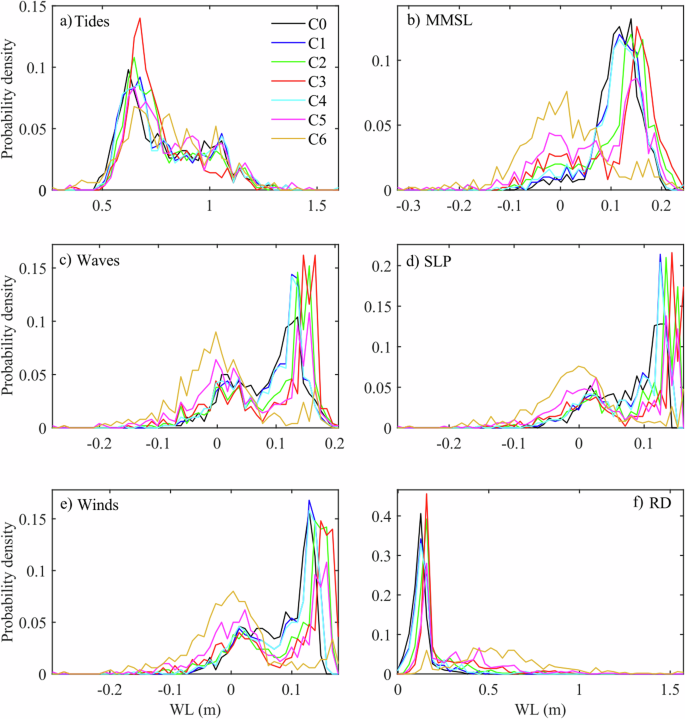
Distributions of WLs associated with the five most extreme events in each simulated hourly 500-year time series due to (a) tides, (b) monthly mean sea level (MMSL), (c) waves, (d) sea level pressure (SLP), (e) winds, and (f) RD under different climate scenarios at location 5 (~26 km from the Delta).

Full size image

The average of the relative contributions of each driver to 100-year return level TWLs across the 100 simulations are calculated under different climate scenarios in the North Bay (i.e., locations 3–9; up to ~55 km seaward of the Delta) (Fig. 5). Either tides or SLR dominate extreme TWLs with relative contributions varying over the climate scenario and/or location. Tides dominate extreme TWLs in the baseline scenario (i.e., C0) and less extreme climate change scenarios with SLR = 0.5 m (i.e., C1 and C4) at all locations. Tides also dominate extreme TWLs under moderate climate change scenarios with SLR = 1.0 m (i.e., C2 and C5) at location 9. SLR dominates extreme TWLs in all the cases when tides do not dominate. Both tides and SLR have a similar contribution to extreme TWLs under the climate change scenarios with the same increase in temperature (also same SLR) but different precipitation rates (e.g., C1 and C4) at all locations except location 3, where the contribution is smaller under C6 than under C3 (Fig. S2). However, the contribution of tides increases seaward in each climate scenario (i.e., C0 − C6) while the contribution of SLR does not vary spatially except in extreme scenarios with SLR = 1.5 m (i.e., C3 and C6) near the Delta.

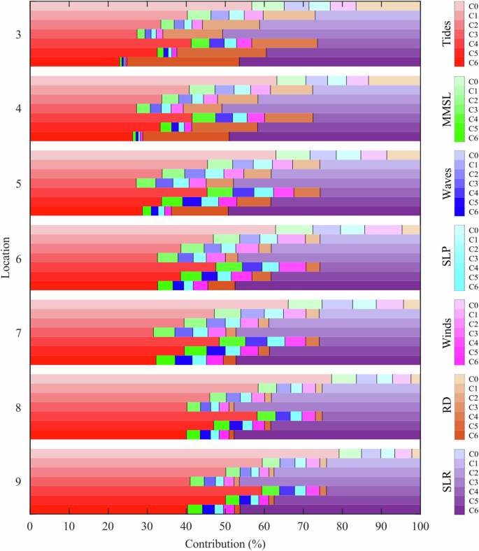
Spatial distributions of the relative contributions of different drivers (i.e., tides, MMSL, waves, SLP, winds, RD, and SLR) to 100-year return level TWLs under different climate scenarios along the centerline of SF North Bay (i.e., locations 3-9).

Full size image

RD has a much larger relative contribution to extreme TWLs than any other non-tidal and non-SLR driver (i.e., MMSL, waves, SLP, and winds), especially near the Delta under more extreme climate change scenarios (e.g., even larger than the relative contribution of tides at location 3 under C6). However, the relative contribution of RD decreases significantly moving seaward, especially under more extreme scenarios (i.e., C5 and C6, Fig. S2). The other non-tidal and non-SLR drivers make a relatively small contribution to extreme TWLs, especially near the Delta under more extreme scenarios (e.g., at location 3 under C6). However, the combined contribution of these drivers (i.e., MMSL, waves, SLP, and winds) can be close to the relative contribution of low SLR (i.e., C1 and C4 when SLR = 0.5 m) at locations 6 and 7 (~32–39 km seaward of the Delta). Furthermore, the relative contributions of these drivers increase from location 3 to around location 6 and then decrease toward location 9 with different variability under different climate scenarios (Fig. S2).

The relative contributions of non-tidal and non-SLR drivers to the non-tidal and non-SLR component of 100-year return level TWLs under different climate scenarios are also investigated (Fig. 6). RD dominates the non-tidal and non-SLR component of extreme TWLs near the Delta, especially under more extreme climate change scenarios (i.e., C0 < C1 < C4 < C2 < C3 < C5 < C6). RD still accounts for around 35% of the non-tidal and non-SLR water level signal, even ~32 km seaward of the Delta (i.e., location 6) under C6. However, the relative contribution of RD decreases significantly moving seaward, and becomes minor and smaller than the other drivers seaward of location 6. Furthermore, the reduction of the relative contribution of RD is projected to be larger under more extreme climate change scenarios (Fig. S3). Each of the other non-tidal and non-SLR drivers has a smaller contribution than RD near the Delta, especially under more extreme climate change scenarios (i.e., C0 > C1 > C4 > C2 > C3 > C5 > C6). In addition, non-tidal and non-SLR drivers other than RD have a similar contribution under the same climate scenario near the Delta, as well as under all climate scenarios seaward of location 6.

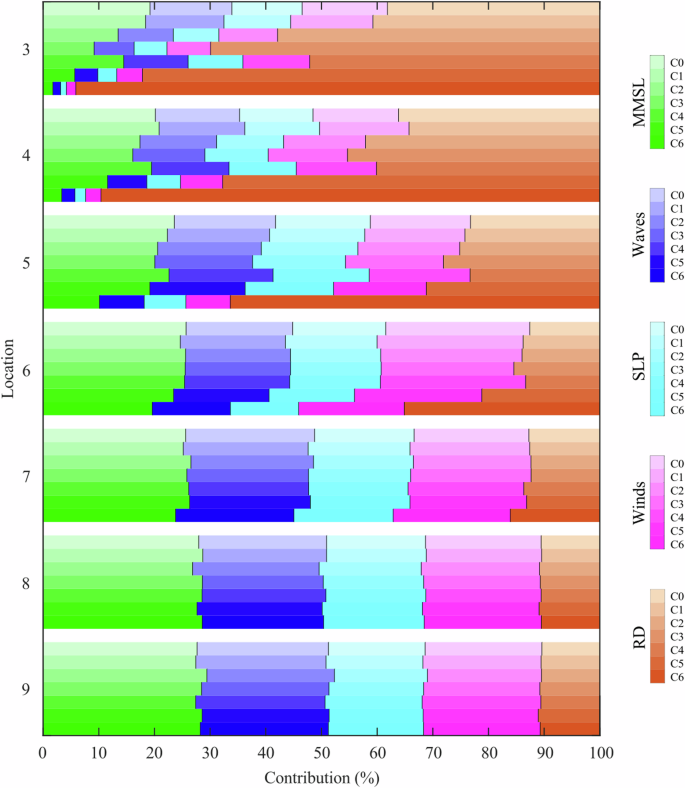
Spatial distributions of relative contributions of non-tidal and non-SLR drivers (i.e., MMSL, waves, SLP, winds, and RD) to non-tidal and non-SLR water levels associated with 100-year return level TWLs under different climate scenarios along the centerline of SF North Bay (i.e., locations 3-9).

Full size image

Compound coastal flooding under climate change poses severe threats globally, including in the SF Bay Area, but is relatively underexplored due to the large sample size needed to analyze extreme events. This study investigates the impact of climate change-induced SLR and increased RD on compound flooding using a hybrid statistical-dynamical approach. The results indicate that climate change could have significant impacts on flood magnitude, frequency, and the relative contributions of different drivers to extreme water levels.

SLR and higher RD due to climate change are projected to result in higher extreme TWLs, which in turn demonstrate different temporal and spatial variability across climate change scenarios and locations within the Bay. The projected rise in sea level will increase water levels by a similar magnitude throughout the entire SF Bay. Higher RD under climate change scenarios (Fig. S4 and Fig. S7) also leads to higher extreme TWLs near the Delta. The variability associated with this driver reduces significantly over distance as downstream TWLs are affected by other drivers, especially tides and SLR.

Climate change is projected to have a significant impact on flood frequency. More extreme climate change with higher SLR and RD will lead to a longer cumulative duration of flood events per year, as SLR and RD will result in more events likely to exceed flood thresholds. In addition, there will be smaller spatial variability of flood frequency (i.e. similar return period) under more extreme climate change scenarios. In this case, special attention should be paid to the parts of the Bay that are more vulnerable to flooding (e.g., the far north and south ends of the Bay¹³) due to potentially higher flood risk in future. Here, the spatial variability analysis is based on existing flood thresholds in the area without considering the change of some important factors such as potential flood defenses over time. A flood thresholding system taking these possible factors into account would result in a more accurate analysis of flood frequency in the Bay and could be used to inform future flood risk reduction at different locations⁵⁸. Previous research shows that extreme flooding associated with 100-year return level events in SF Bay can become annual events by the end of this century³. The present study shows that the situation can become even more severe. For instance, major flood events are projected to occur annually under the climate changes scenarios with SLR = 1.5 m (i.e., C3 and C6) while they occur only once every few hundred years under the climate changes scenarios with SLR = 0.5 m (i.e., C1 and C4). It is clearly important to reevaluate the return period of coastal flood events in SF Bay to understand the change in risk under climate change³⁰.

The relative contributions of each forcing driver to extreme TWLs are projected to change with climate change. In this study, climate change impacts only mean sea level (via SLR) and RD. However, the similar order of magnitude for the non-tidal and non-SLR drivers other than RD (i.e., MMSL, waves, SLP, and winds) under all climate scenarios confirms that each of these drivers is also important for the extreme TWLs in SF Bay⁵⁶. The WLs due to SLR or RD have a larger range under more extreme climate change scenarios. The minimum WLs associated with RD will be similar under all assessed climate scenarios while the maxima will be larger under more extreme climate change scenarios. This can be clearly seen from the correlation between extreme TWLs and their associated RD in more extreme climate change scenarios, especially for the Sacramento River near the Delta (location 3 in Fig. S5). Note that the correlation does not necessarily become stronger under a more extreme climate change scenario (e.g., Sacramento River under C5 − C6 at location 3). The WLs due to non-tidal and non-SLR drivers other than RD shift to a smaller magnitude while the WLs associated with RD shift to a larger magnitude under more extreme climate change scenarios. This observation and the finding of the correlation between extreme TWLs and their associated RD confirm the finding that extreme compound flood events are not necessarily the result of all individual drivers being extreme, but instead can occur over a wide range of driver combinations^45,59. In this context, high-fidelity but compute-intensive dynamical approaches or compute-efficient statistical approaches (e.g., joint probability analysis) without sufficient historical data do not necessarily capture extreme compound flood events by assuming that extreme flooding is induced by a particular forcing combination with extreme values of drivers^8,45. The hybrid statistical-dynamical approach with accuracy similar to dynamical approaches but much higher computational efficiency⁵⁶ is able to characterize extreme compound flooding by exploring the full range of possible forcing combinations under stochastic climate and weather conditions at any location of interest.

Climate change is projected to have a significant impact on the spatial distribution of the relative contributions of each driver to extreme TWLs, and of non-tidal and non-SLR drivers to the non-tidal and non-SLR components of extreme TWLs. Tidal dominance to extreme TWLs will be reduced due to greater contributions of SLR and river discharge near the Delta under a more extreme climate change scenario, especially when high SLR coincides with high river discharge. However, the relative contribution of tides increases seaward under all assessed climate scenarios due to decreasing relative contribution of river discharge, resulting in tidal dominance to extreme TWLs far away from the Delta under moderate climate change scenarios. This highlights the importance of tides to extreme TWLs in SF Bay under both today’s climate and future climate scenarios^56,60. SLR is expected to dominate extreme TWLs throughout the Bay in more extreme climate change scenarios, even when river discharge is extremely high. The contribution of SLR to extreme compound flooding found here aligns with previous research on SF Bay and other coasts around the world^23,24,61,62.

Increased intensity of precipitation due to climate change, along with a shift from snow to rain during the winter, will cause greater peak river discharge into SF Bay and increase extreme TWLs. Due to the impact of other forcings (tides and SLR in particular), the relative contribution of the downstream discharge of the river becomes limited and even smaller than other non-tidal and non-SLR drivers, although it has significant consequences on compound flooding on the upstream boundary⁵¹. Note that river discharge can dominate the non-tidal and non-SLR water level signal throughout approximately half of the North Bay (i.e., locations 3-6) under the extreme climate change scenario. This result demonstrates the great impact that river discharge could have on compound flooding and highlights the importance of combining a stochastic weather generator^63,64,65 with a hydrologic and reservoir system model^66,67) (i.e., the two modules composing the hybrid statistical-dynamical approach⁵⁶). While this analysis assumes that the upstream reservoir system maintains current flood control operations in the future, this may be a key opportunity for adaptation to reduce the river discharge component of compound flooding in the Bay⁶⁸. The hybrid approach can generate the full range of possible river discharges that may contribute to extreme compound flooding events under stochastic climate and weather conditions. The non-tidal and non-SLR drivers other than river discharge are not negligible in compound flooding analysis, especially in the cases with minor relative contribution of river discharge and low SLR. The impact of climate change on the spatial distribution of the relative contributions of the drivers not only indicates the need to evaluate these relative contributions in the analysis of compound flooding under climate change^8,69, but also confirms the impact of climate change on the complex compounding interactions of the flood drivers^{23,51,61,62,70}.

More research on compound coastal flooding under climate change will improve adaptation planning for climate change in the Bay Area. For example, compound flooding analysis under additional climate change scenarios that consider mean precipitation increase to reflect more precipitation falling as rain instead of snow could inform the investment in water resources systems to adapt to extreme precipitation events. Incorporating the impact of climate change on additional forcing parameters such as the wind and wave climate would result in a more comprehensive investigation of future changes to flooding in the region. While many important uncertainties associated with climate and weather variability as well as TWL forcing are captured here, other uncertainties associated with TWL forcing (e.g., non-stationarity of forcing variables), model parameters (e.g., roughness coefficient in the hydrodynamic model), and model structure (e.g., a priori assumptions of underlying processes) can also impact the TWL variability⁷¹. Advanced statistical methods such as data assimilation may be employed to account for these uncertainties to improve the extreme TWL estimates using surrogate models based on new observed data⁷¹. In addition, a compound flood risk analysis under climate change that accounts for flooding, exposure (e.g., building properties), and vulnerability (e.g., flood fragility) will provide important information on flood risk management in the Bay Area. This can be accomplished through coupling the hybrid statistical-dynamical framework with the exposure models (e.g., modeling of building properties), vulnerability models (e.g., flood fragility function), and risk assessment models (e.g., risk quantification).

Our compound coastal flooding analysis in SF Bay under climate change reveals that SLR and higher RD would lead to more extensive and frequent coastal flooding, to which the Bay’s shoreline and flood protection infrastructure will become increasingly exposed. This finding has important implications for planning and design to reduce the risk of flooding^2,3. The flooding analysis also shows that climate change could have a significant impact on the relative importance of drivers to extreme compound flooding, which is crucial for understanding the evolution of compound flood risk to cope with climate change²⁹. In addition, this study has revealed that climate change could greatly influence the spatial variability of flood magnitude and the relative contributions of drivers in the North Bay (especially near the Delta), and the spatial variability of flood frequency in the Bay. These results are particularly useful for identifying trigger points for the implementation of climate adaptation strategies to improve coastal resilience².

Hybrid statistical-dynamical framework

The hybrid statistical-dynamical framework for compound coastal flooding analysis is developed by integrating a stochastic generator of compound flooding drivers, a physics-based high fidelity hydrodynamic model, and machine learning-based surrogate models⁵⁶ (Fig. S6). The generator of compound flooding drivers can simulate time series of joint astronomic, atmospheric, oceanographic, and hydrologic forcings of compound coastal flooding in SF Bay by combining a sea surface temperature (SST) reconstruction model⁷², a stochastic climate emulator⁷³, a stochastic weather generator^63,64,65, and a hybrid physics-based and data-driven hydrologic and reservoir system model^66,67). The SST reconstruction model⁷² creates the annual principal components (APCs) of SST anomalies, which are passed into the climate emulator TESLA (Time-varying Emulator for Short- and Long-Term analysis)⁷³ to generate synthetic annual weather types (AWTs). TESLA also simulates synthetic intraseasonal weather types (IWTs) based on variability of the Madden-Julian Oscillation. Synthetic daily weather types (DWTs) are created which are conditionally dependent on the IWTs and AWTs. The hourly time series of multiple drivers of compound coastal flooding (i.e., MMSL, waves, SLP, and winds) are generated from synthetic DWT time series. The weather generator^63,64,65, hydrologic model⁶⁶, and reservoir system model⁶⁷ are combined under the same DWTs simulated by TESLA to generate the daily time series of RD. Note that deterministic astronomical tides are simulated using the UTide model⁷⁴.

A hydrodynamic model is developed to run a relatively small library of simulations with boundary conditions defined by representative samples for compound flooding drivers, which are generated using the Maximum Dissimilarity Algorithm (MDA)⁷⁵. The D-Flow Flexible Mesh (D-Flow FM) model adapted from ref. ⁸ by simplifying grid and boundary conditions is coupled with a wave model based on Simulating WAves Nearshore (SWAN)⁷⁶ to develop a Delft3D FM (D3D FM) coupled flow-wave model for the simulation of TWLs throughout SF Bay.

Based on the relatively small number of D3D FM coupled flow-wave model simulations, optimized Gaussian process regression (GPR) surrogate models are developed using five-fold cross-validation^40,54 to efficiently simulate WLs driven by all or some of the flooding drivers at each of locations 3–18 shown in Fig. 1.

The validation of each model/emulator that makes up the generator of compound flood drivers is documented in detail in refs. ^{63,64,65,66,67,72,73}, and the validation of the D3D FM coupled flow-wave model and the GPR model can be found in ref. ⁵⁶. In addition, the five-fold cross-validation of the GPR model in all scenarios with and without climate change is provided in Table S4. The validated hybrid statistical-dynamical framework is employed to efficiently run 100 500-year hourly simulations representing the full range of possible forcing combinations under all considered climate scenarios, from which the predicted hourly water levels at locations 3–18 along SF Bay center line are used for compound flooding analysis.

Climate change scenarios

Here, climate change in SF Bay is reflected by warmer temperatures and a change in the hydrological cycle¹¹. The former results in SLR¹¹ and higher precipitation rates^11,18, while the latter leads to more precipitation falling as rain instead of snow¹⁸. Higher precipitation rates and more precipitation occurring as rain causes higher peak RD flowing into the Bay from Sacramento and San Joaquin rivers. Six scenarios of climate change affecting temperature, average precipitation, and extreme precipitation (i.e., C₁–C₆ in Table S1) of the weather generator simulation for CA^64,65 are selected for flood analysis over a period of 500 years. These include one baseline scenario with no climate change (C₀), and three possible warming scenarios (i.e., warming of 1°C, 3°C, and 5°C) each with no mean precipitation change but two levels of thermodynamic scaling rate of 7% and 14% per ◦C, which replicate the effects of warming temperatures on precipitation through increases in the moisture-holding capacity of the atmosphere. Note that the stochastic weather generator uses a bottom-up approach with a higher computational efficiency compared to traditional top-down approaches such as global climate models (GCM) and ensures a thorough exploration of the system sensitivity to small perturbations in climate, which might be missing when employing a relatively small and often biased GCM ensemble. Also, the weather generator can use GCM-based information to inform the range of possible future climate changes and their probability. More details on the development of climate change scenarios with stochastic weather generators can be found in refs. ^63,64,65. The local SLR scenarios are linked to increasing temperatures by assuming an approximately linear relationship between the global SLR (GSLR) and the increase in mean temperature^33,77,78, and a local SLR rate similar to the global average SLR rate^16,79. Here, three possible sea level scenarios with GSLR values of 0.5 m (Intermediate-Low), 1.0 m (Intermediate), and 1.5 m (Intermediate-High) that account for the uncertainty of the process and emissions in ref. ⁸⁰ are linked to the temperature increase of 1°C, 3°C, and 5°C, respectively. In addition, a baseline scenario without climate change (i.e., C₀ without SLR and precipitation change) is defined for comparison in the same period. The distribution of RD under each climate scenario is calculated (Fig. S7) based on all the minima, 10^th,…, 90^th percentiles, and the maxima of each simulated hourly 500-year time series to support flooding analysis.

Flood metrics

We consider three compound coastal flood metrics including flood magnitude, flood frequency, and the relative contributions of drivers to extreme flood events because they can provide important information about extreme events to improve flood protection and coastal resilience^2,8,41,45,49. Flood magnitude is quantified by 100-year return level TWL events, which are identified based on annual maximum TWLs (the fifth largest annual maxima in the 500-year time series). The frequency of occurrence of water levels exceeding flood thresholds for nuisance, minor, moderate, and major flooding^56,57,58 is calculated based on the exceedance probability of annual maximum TWLs. The minor, moderate, and major flood thresholds at NOAA gauges are estimated based on a linear regression between the tide range and NOAA flood threshold derived in ref. ⁵⁷. The median nuisance flood thresholds at locations 7-18 are estimated based on the latest threshold ranges⁵⁸. Flood frequencies at each of locations 3–18 are calculated based on the median nuisance flood threshold at the closest location and the minor, moderate, and major flood thresholds at the closest NOAA gauge. Note that nuisance flood thresholds at locations 3–6 are estimated using linear extrapolation based on nuisance flood thresholds at other locations (7–18) and the distributions of minor, moderate, and major flood thresholds across locations 3–18. Here, nuisance flooding is viewed as being less severe than minor flooding.

At each location, the relative contributions of different forcings to return level events are estimated by dividing the extreme TWL by the WL due to each individual driver. Tidal water levels are calculated by running the GPR model only with tidal drivers as input⁵⁴. The WL due to each non-tidal driver is then estimated by first running the GPR model by excluding this driver and then subtracting the predicted WL from the extreme TWL. The WL due to each non-tidal and non-SLR driver that is associated with the return level events is divided by the sum of these WLs to obtain the relative contributions of non-tidal and non-SLR drivers to the non-tidal and non-SLR component of return level events. Please refer to ref. ⁵⁶ for more details on the definition and calculation of the three flood metrics. All metrics are quantified based on the 100 hourly 500-year water level time series that fully capture the parameter space of compound flooding under different climate change scenarios. Note that all WLs are relative to mean sea level (MSL).

Data

The main input and output data for each model component of the hybrid statistical-dynamical framework are provided in the Supplementary Data section in ref. ⁵⁶. The detailed underlying data requirements of the compound flooding drivers generator can be found in each published model/emulator, i.e., the SST reconstruction model⁷², climate emulator (TESLA)⁷³, weather generator^63,64,65, hydrologic model⁶⁶, and reservoir system model⁶⁷. To build the D3D FM coupled flow-wave model, please refer to ref. ⁸ for the full description of data inputs for the flow model. The wave data for the development of TESLA is used to force the SWAN wave model. The D3D FM coupled model and the GPR surrogate models are validated using the same data set, i.e., hourly time series of all considered compound flood drivers and the corresponding hourly TWLs time series observed by NOAA (i.e., 2008-2018). Note that 500 years of historical proxies (i.e., tree-ring, corals, and sclerosponge-based El Nin˜o Southern Oscillation-ENSO reconstructions) are used to feed the generator of compound flooding drivers under the consideration of climate change to generate the 100 simulations of hourly 500-year non-tidal and non-SLR forcing combinations. Together with the hourly tides and the SLR values considered during the 500 years, the 100 hourly 500-year time series of forcings are input into GPR surrogate models to predict hourly water levels to capture extreme compound flooding up to a 500-year return period for flooding analysis.