Continous–discontinous analysis of an unstable slope: evolution of damage zones and potential influencing areas

Introduction
Landslides commonly happen in China annually1. Many landslides evolve from unstable slopes that contain faults or weak layers2,3,4. Some of these slopes are characterized by long-term creep before the sudden slide. For example, the Niuerwan slope in Chongqing experienced continuous deformation since 1998 till its failure in 2020, which was induced by rainfall. This landslide finally destroyed eight houses, two main roads, and a shale gas pipeline5. At present, many slopes exhibiting long-term creep require risk assessment and remediation. In 2023, surveyors found that the Zhutou slope in Nanjing was in the creep deformation stage. The maximum cumulative displacement for the entire year reached 410.3 mm. The potential landslide threatens the safety of the surrounding inhabitants and industrial buildings, requiring stability assessment and disaster analysis of this slope.
Research methods for landslide include empirical statistical methods6,7,8, experimental investigations9,10, and numerical simulations. Compared to empirical statistical methods, numerical analysis allows for flexible parameter settings to achieve more accurate results. In contrast to physical experiments, numerical analysis is cost- and time-efficient, which becomes very importance research method in recent years. However, numerically simulating the whole failure process of slopes is a challenging task, which refers to stability analysis before failure and large deformation analysis after11,12. For the former process, Finite Element Method (FEM) is commonly used to determine the factor of safety, quantifying the stability state and corresponding damaging zones based on elastoplastic analysis13,14,15,16. As a continuous-based approach, FEM is less applicable for large deformation analysis comparing to discontinuous-based method such as Smoothed Particle Hydrodynamics (SPH)17,18,19, Material Point Method (MPM)20,21,22,23, Computational Fluid Dynamics (CFD)24,25,26, Discrete Element Method (DEM)27,28,29, and Discontinuous Deformation Analysis (DDA)30,31,32. Many of these methods focus on the interacting forces between discretized blocks and particles, which are advantageous in handling large displacements and deformations of slopes33. However, current research lacks comprehensive methods that can handle both the stability analysis before failure and the large deformation analysis after failure. Moreover, these researches mostly relied on two-dimensional models, which are unable to provide a comprehensive representation of the slope in the natural terrain, making it difficult to evaluate the morphology of the potential sliding mass and its influencing areas. The Continuum-Discontinuum Element Method (CDEM) is a hybrid finite-discrete element method. In CDEM, the caculation domain is discretized by deformable blocks and interfaces. The CDEM has been well-known used in simulating three-dimensional discontinuous deformation problems34,35 such as landsides, capturing the elastoplastic deformations, rupture, sliding and rolling of slope blocks36. Although CDEM has achieved certain success in landslide simulations37,38,39, research integrating hydro-mechanical couping effects into these simulations remains limited. External factors, such as groundwater, significantly influence water flow within the slope, affecting soil strength and the potential volume of landslides40,41. Additionally, the selection of particle flow parameters in CDEM is a complex issue. Further exploration and optimization are still required to determine how to appropriately select particle flow parameters based on soil properties and external environmental conditions.
In this study, the stability and potential disaster areas of Zhutou slope were evaluated with CDEM through a 3D model. To accurately simulate the response of the slope under hydro-mechanical coupling effects, we optimized the seepage process by incorporating an unsaturated soil model, and simulated the strength reduction of the weak layer under groundwater seepage. The damage zones and safety factor of the slope were evaluated using the strength reduction method. After determining the damaging zones, the particle flow method was used to simulate the large deformation process of the slope. The parameter setting for the particle flow simulation were calibrated through direct shear tests. Considering the different fluidity of the landslide mass, the potential influencing areas were predicted.
The structure of this paper is as follows. Firstly, the overview of Zhutou slope is briefly introduced in Sections “Study area” and “Deformation phenomena”. Then in Sections “Basic conception of CDEM”, “Optimized seepage model” and “Particle flow model”, the basic theory of CDEM, optimized seepage, and particle flow are introduced. In Sections “Results”, stability and large deformation analysis are conducted, revealing the evolution of the damage zone and capturing the whole failure process. Finally, discussions are provided in Section “Discussion”.
Methods
Study area
Zhutou slope is located in Nanjing (longitude 118°39’30” East, latitude 32°09’22” North), Jiangsu Province, China (Fig. 1), which is recognized as the largest potential landslide in Nanjing. Considering its shape, the south part is around 100 m higher than the north part. The southern region comprises the uplifted hills of the Laoshan area, with the mountain range extending in a northeast direction. The northern region is alluvial plain of the Chu River. The study area features an eroded and accumulated hilly landscape, belonging to the geological structural unit under the Yangtze platform. In addition, this region is a component of the Yangtze platform’s fold belt, where folds and faults are developed (Fig. 2).

This figure presents a location map and an aerial overview photograph of the study area taken in 2019. The map provides geographical context, while the photograph illustrates key landscape features pertinent to the study.
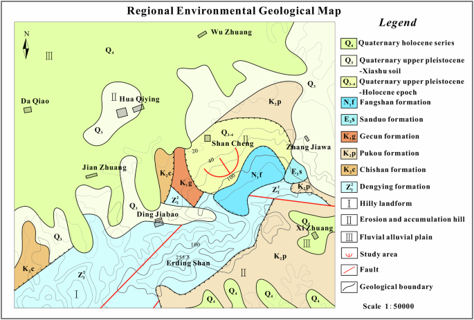
This geological map outlines the various rock and soil formations within the study area. Key geological structures and faults are marked to aid in understanding the area’s characteristics.
Based on existing data, the soils and rocks around the study area can be categorized into five layers according to the sedimentary age and genesis (Fig. 3). The first layer consists of fill soil formed by accumulation during sand extraction processes. The second layer consists of Quaternary Upper Pleistocene Xiashu loess, which contains a substantial amount of kaolin. The third layer is the Dongxuanguan Formation sand layer from the Upper Tertiary Middle Series. The fourth layer consists of semi-lithified sandy mudstone. In addition, on the southern part of the slope, basalt from the Fangshan Formation is distributed. During the rainy season, rainfall flows along the tectonic and weathered fissures in the basalt into the sand layer. Once the sand layer becomes saturated, the water begins to seep upward. Because of the relatively high content of kaolin in the clay layer, it has low shear strength and easily softens when in contact with water. Under the action of dry and wet circulation of groundwater, its mechanical strength keeps decreasing over time. Furthermore, with the presence of vertical joints in the clay layer locally, it is highly prone to deformation. According to the field engineering geological survey and investigation data, the sliding surface is at the junction of the clay layer and the sand layer. The rear edge of the landslide is near the Fangshan Formation basalt, while the front edge is located at the pinch-out part of sand layer, see Fig. 3. In the past twenty years, study area has experienced four small slides, occurring after heavy rainfall. After the landslide occurs, the slope will still be in creep. The width and length of the cracks on the ground gradually increase. The landslide scarp at the rear edge of the slope keeps growing larger, showing a state of creeping deformation. Its future deformation and destruction pattern is collapse-crack and creep-crack type. Heavy rains may trigger slope sliding again, directly threatening the safety of lives and properties near the foot of the slope.
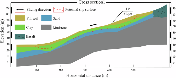
This diagram provides a detailed cross-sectional view of the study area, illustrating the position of the sliding surface, slope angle and soil compositions along Cross-section 1.
Deformation phenomena
By field investigations, three hazardous areas, HP01, HP03 and HP04, have been identified, see Fig. 4a and Table 1. The primary sliding direction of HP01 is northwest (NW) at 330°, with the potential landslide extending approximately 300 m in width and 400 m in length, covering an area around 120,000m2. The average thickness of the sliding body in this area is about 10 m. Regarding to the deformation of HP01, tensile cracks emerged at the rear edge of the slope, with the height difference of the landslide scarp ranging from 1 m to 1.5 m, see Fig. 4c. In the middle part of HP01, a wide range of cracking and deformation occurred on the ground surface. As depicted in Fig. 4b, the existing anti-slide piles have been squeezed and deformed. Continuous deformation has transformed this area into a gully. Furthermore, the shear outlet can be observed at the foot of the slope, the soil at this area has uplifted by 0.5 m to 1 m, see Fig. 4e. The main sliding direction of HP03 is NW320°, with a width of 110 m, length of 200 m, and an area of 22,000m2. The average thickness of the sliding body in this area is about 10 m. The rear edge of HP03 is located next to the shooting range. Notable cracks have been found on the retaining wall, the offset of some cracks exceeds 1 m, see Fig. 4d. The main sliding direction of HP04 is NW320°, with a width of 80 m, length of 100 m and an area of 8,000m2. The average thickness of the sliding body in this area is about 5 m. At the foot of HP04, where the ground is the road inside the shooting range, the drainage ditches have been severely deformed due to lateral pressure, see Fig. 4a.
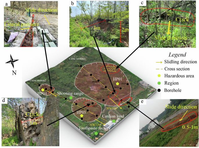
a Squeezed deformation of drainage ditches. b Gully (originally a crack behind the anti-slide pile). c Residual rear edge of HP01. d Cracks in the retaining wall. e Obvious uplift of soil at the foot of HP01. Preliminary field investigation results were collected for the study area, analyzing the typical damage characteristics at various locations. Among them, a Squeezed deformation of drainage ditches at HP04. b Gully formation, originally a crack behind the anti-slide pile at HP01, c Residual rear edge of HP01, d Cracks in the retaining wall at HP03, with offsets exceeding 1 meter, e Noticeable uplift of soil at the foot of HP01.
Basic conception of CDEM
The Continuum-Discontinuum Element Method (CDEM) is a numerical algorithm combing finite and discrete element methods, specialized for simulating the progressive failure of materials in geotechnical engineering37,42. Through the Lagrange energy system, control equations are built as
where ({u}_{i}) and ({v}_{i}) represent generalized coordinates, ({Q}_{i}) denotes the work done by non-conservative forces, and (L) is the Lagrange function, described as
where ({varPi }_{m}), ({varPi }_{e}), and ({varPi }_{f}) represent the system’s kinetic energy, elastic energy, and the work of conservative forces.
The dynamic equation for CDEM is
where (ddot{u}), (dot{u}), and (u) represent the acceleration, velocity, and displacement arrays of all nodes within the element, and M, C, K, and F denote the element’s mass matrix, damping matrix, stiffness matrix, and external load array.
Optimized seepage model
This study captures the seepage processes by incorporating an unsaturated soil model. An explicit solution technique is used in the seepage process. The finite volume method is used to obtain the water pressure in rock mass43,44. In each time step, the saturation and pore water pressure for each node are derived from the nodal flow rate. The saturation (s) of node is calculated by
where (s) is the saturation, (n) is the porosity, (V) is the total volume of the node, ({Q}_{{app}}) is the flowrate boundary, (Q) is the total flow of the node, and (varDelta t) is the calculation time step. When the node saturation accumulates to 1, the pore water pressure ({p}_{p}) is calculated as
where ({K}_{f}) is the bulk modulus of the fluid.
When the average saturation of block is equals 1, the total pressure (P) at any node within the block can be described as
Where ρf is the density of water, x, y, z are the global coordinates of a node within the block, gx, gy, gz are the components of the global gravitational acceleration, respectively, (bar{s}) represents the average saturation of the block.
When the average saturation of block is less than 1, an unsaturated soil model proposed in literature45 is used to describe the change in shear strength of unsaturated soil:
where ({S}_{{rm{rc}}}) is the saturation level when the soil’s internal friction angle begins to increase, defined as the critical saturation; ({varphi }^{{prime} }) is the mean value of the soil’s internal friction angle when ({S}_{{rm{r}}}ge {S}_{{rm{rc}}}), approximately equal to the internal friction angle of saturated soil (°); ({varphi }_{{rm{d}}}) is the maximum internal friction angle (°) of the unsaturated soil.
The cohesion varies with saturation as described by a piecewise function model:
where (a), (b), (d) are fitting parameters; ({c}_{d}) is the cohesion of the soil when ({S}_{{rm{r}}}=0); ({S}_{{rm{rV}}}) is the saturation corresponding to the maximum cohesion of unsaturated soil.
Particle flow model
Particle flow method is adopted to predict the influencing areas of the potential landslide. When simulating large deformations of the slopes, contact relations among particles and blocks are built by global and local contact search algorithms, which ensuring identification across particles-points, particles-edges, and particles-surfaces46, see Fig. 5a. When detecting contact between two particles/blocks, contact constitutive relations are introduced and contact forces will be obtained, see Fig. 5b.
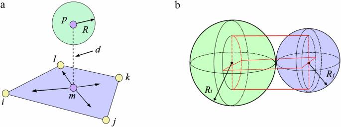
a Contact detection between particle and block. b 3D model of particle contact key. a, b Displays contact detection between particles and blocks, helping to understand the contact mode in particle flow model.
The normal and shear contact force on each contact key is calculated by incremental method47,48
where Fn and Fs are normal and shear contact force; kn and ks are normal and shear contact stiffness (Pa/m); ({A}_{c}) is the cross-sectional area of contact key; Δdun and Δdus are the increments of normal and shear displacements. The following equation is used to determine tensile failure and correct the normal contact force upon tensile failure:
where ({sigma }_{n}) is the normal stress of the contact key; ({sigma }_{t}) is the material’s tensile strength (units: Pa). The following equation is used to determine shear failure and correct the tangential force of the contact pair upon shear failure:
where (phi) is the internal friction angle of the contact key; (c) is the material’s cohesion.
Results
3D geological model
A high-resolution 3D geological model was constructed for this study, see Fig. 6. Firstly, the surface was modeled based on laser point cloud data which were captured via drone-obtained oblique photography. The thickness of the clay and the sand were determined by the observation and analysis from the borehole tests. The borehole data was imported into Rhino, which proceeds pinch-outs and lenticular bodies and generates a stratigraphic model by classifying sub-layer formations according to stratigraphic unit numbers. The locations of the boreholes can be seen in Fig. 4. Following this, the bedrock was modeled based on the upper boundary data of mudstone and basalt obtained from the HVSR microtremor surveys. However, since the strength of rock is far greater than that of soil, and the influence of rock fissures on slope stability was not considered in the numerical simulation, basalt was regarded as mudstone during the modeling process. Three software (Rhino, Ansys, and Gid) were used to produce the 3D model, giving the discretized domain with tetrahedral elements. The layers of the model from top to bottom are filled soil, clay, sand and mudstone.
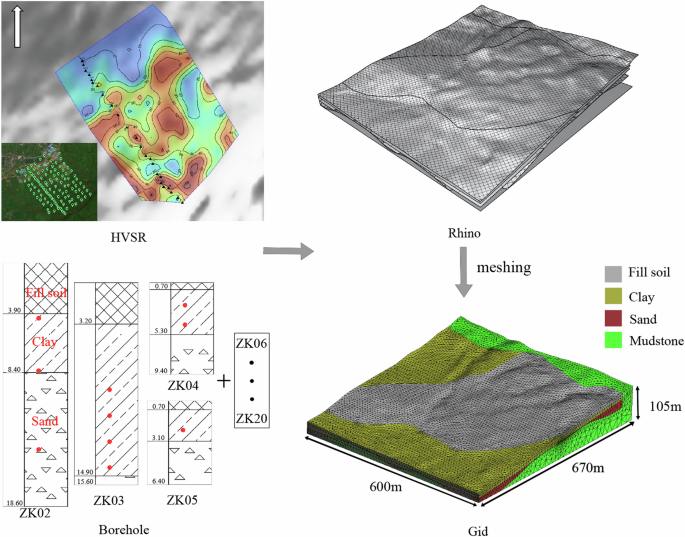
The figure shows the modeling process of Rhino and Gid, and shows the distribution of the soil layers.
Parameters of soils
In the simulation, the Mohr-Coulomb strain-softening model was used to describe the constitutive relationship of the soil. Borehole reports show that during the rainy season, the stabilized groundwater table is located in the sand layer, which is set at the bottom of the clay layer. The values for all soils are given in Table 2 and Table 3, obtained from the Nanjing Geological Engineering Survey Institute Testing Center. For the values of the unsaturated soil parameters ({S}_{r{rm{v}}}) and ({S}_{{rc}}), we referred to experimental data from Gong49, which includes over 2000 soil samples from more than 100 different clay soils. The mean values were fitted using the unsaturated soil shear strength functions presented in Eqs. (7) and (8). As shown in Fig. 7a, the ({S}_{{rc}}) value for clay is typically 0, indicating that the cohesion of clay gradually decreases with increasing saturation, which is consistent with the findings of Zhao45. To ensure the broad applicability of ({S}_{{rv}}), we further collected clay samples from several regions in China and fitted the data with the function. As shown in Table 4, the value of ({S}_{{rc}}) ranges from 0.45 to 0.65. Therefore, the Src value is set to be 0.55 (Fig. 7b), which effectively represents the behavior of the majority of clay samples. Moreover, given the analogous granulometric composition and mechanical properties between the fill soil and the clay soil, the unsaturated soil parameter of the fill soil is assigned the same values as clay. The values for sand and mudstone are assigned based on the experimental data.
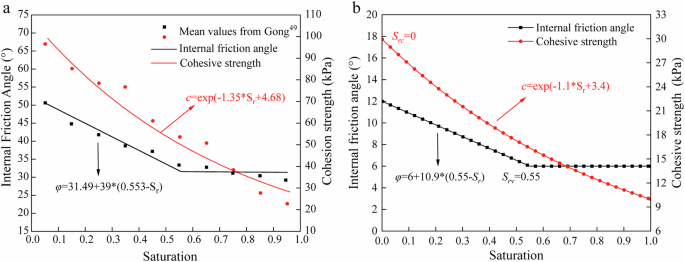
a Shear strength variation curve for clay, showing the mean values from Gong49, fitted through the function used in this study. b Shear strength variation curve for clay, illustrating the relationship between shear strength and saturation.
Stability analysis and damage zones
The strength of the clay layer plays a critical role in the stability of Zhutou slope. According to Section “Study area”, rainwater will flow into the sand layer during the rainy season, raising the groundwater level and softening the clay and fill layer. Therefore, numerical simulations were conducted with the groundwater level applied beneath the clay layer to assess its impact on slope stability. Under the influence of groundwater seepage, the saturation of fill soil and clay gradually increases, see Fig. 8a. Fill soil and clay tends to soften upon contact with water. As the increase of saturation, the strength of the soil gradually decreases. This resulted in decreases in the c and φ values for a portion of the soil. The decreases in effective cohesion and internal friction angle of the soil are shown in Fig. 8b, c. After seepage, the weak interlayer softens and its position becomes more apparent. Concurrently, the maximum displacement occurs on the surface of HP03, with a value of 0.3039 m (Fig. 8d). A large area of displacement also appears at HP01, posing a serious threat to the stability of the slope.
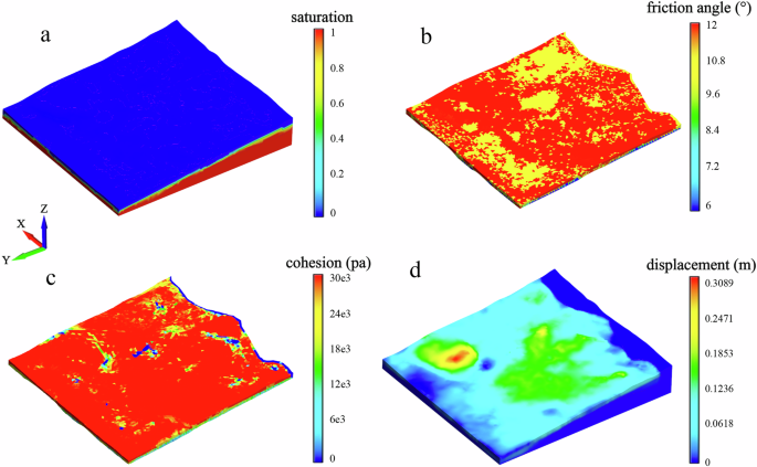
a Saturation distribution after seepage. b Effective friction angle of unsaturated soil. c Effective cohesion of unsaturated soil. d Displacement after seepage. a Displays the distribution of soil saturation after seepage. b, c Shows the effective friction angle and effective cohesion of unsaturated soil after seepage, revealing the landslide mechanism, d Shows the impact of seepage on soil displacement.
In the stability analysis, two criteria were used to assess whether a slope fails. The first is to determine whether there are significant displacements in the slope, and the second is to check whether the tensile shear damage zones have developed along the potential slip surface. If either of these conditions occurs, the slope is considered to have failed.
As shown in Fig. 9a, the results show that the safety factor is 1.24. According to “The technical code for building slope engineering (GB50330-2013)”, a slope is considered unstable if its FOS is less than 1.35. As shown in Fig. 9b, c, the number of damaged blocks increases as the strength decreases. This process gradually reveals the contour of the landslide, with the Zhutou slope exhibits mid-shallow landslide, see Fig. 10a–d. The tensile-shear damage zones are mainly distributed on the north and southwest sides of the shooting range and above the Canlian land in the central part of the investigation area. Comparing the results of the damage zones with the displacement, it is clear that the damage zones correspond to areas of large deformation (Fig. 9d). By using the shape and position of the damaged blocks as the boundary of the large deformation zone, and the enclosed mass as the potential landslide mass, the potential landslide volume is measured about 2 million m³ (Fig. 9e, f). The potential landslide volume of HP03 is larger than that of field investigation, which may be due to the fact that reinforcement measures such as anti-slide piles and retaining walls were not considered during the simulation. Nevertheless, the location and shape of the damage zones are generally consistent with the field investigation.
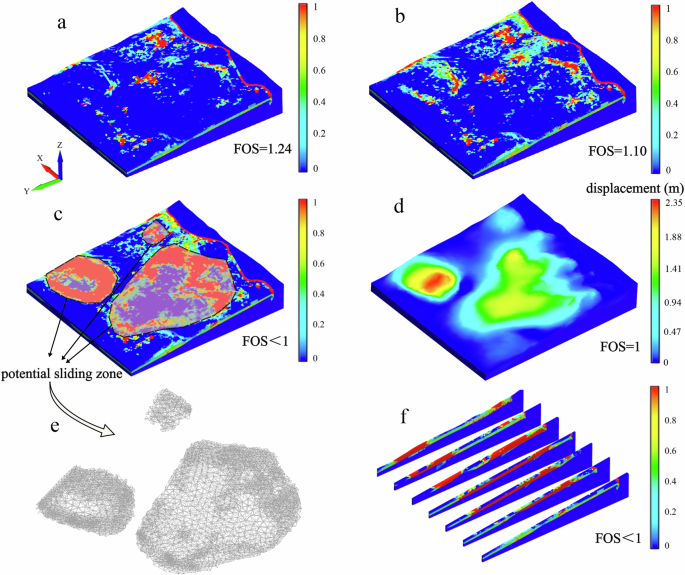
a–c Distribution of tensile-shear damage zone at different FOS. d Deformation at FOS = 1. e Damaged blocks. f Profile diagram of tensile-shear damage zones (reaching 1 represents the occurrence of tensile or shear damage). a–c Displays tensile-shear damagezones at different FOS, analyzing the relationship between damage zones and FOS. d Determines the failure range when the FOS = 1 and identifies the location of unstable blocks. e, f Provides a visual representation of potential hazard areas on the slope.
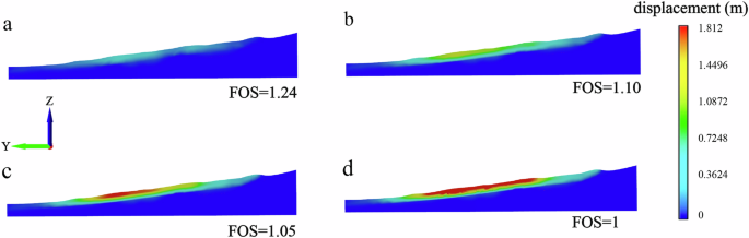
a–d Displacement in section 1 under different FOS. a–d Panel a shows the displacement for FOS = 1.24, Panel b shows the displacement for FOS = 1.10, Panel c shows the displacement for FOS = 1.05, Panel d shows the displacement for FOS = 1.
3D particle-block model and monitoring point
In the above analysis, the shapes and locations of the potential landslide have been determined. According to the results of laboratory geotechnical tests, 79.9% of the soil particles range from 0.075 mm to 0.75 mm, 6.7% range from 0.1 mm to 0.075 mm, and 13.4% are smaller than 0.075 mm. We applied the equivalent substitution method to consolidate the particle size distribution into the 0.075–0.75 mm range50,51. This approach retains the original gradation in the study scale to decrease computation. Additionally, the number of particles in the DEM simulation is constrained by software and computational limitations. When the particle count in the simulation is significantly lower than in reality, larger particle sizes are necessary to complete the simulation. To minimize size effects and obtain macroscopically representative results, the REV size should be at least seven to eight times the maximum particle size52. The GID software was used to post-process the unsafety blocks, 12471 particles with a radius from 0.5 to 5 m and a volume of 1.2 million m³ were generated. Additionally, the particles from the front, middle and rear of the sliding body were selected for monitoring, see Fig. 11. The material parameters are given in Table 5, and the contact parameters between particle and block inherited from the sliding mass. The kinetic energy of the particle ({KE}) is taken to quantify the destructive potential, calculated by
where ({m}_{i}),({v}_{i}), and (N) are the mass, the average velocity, and the total number of the particles.
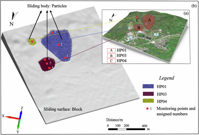
Shows the region of particle flow modeling and identifies the location of each monitoring point.
Calibration of the particle parameters
The macroscopic mechanical properties of soils are characterized by the combination of macro and micro parameters of particles. A 3D direct shear test was constructed to calibrate the parameters. The direct shear model is a cube with a side length of 10 cm, with boundary walls extends 2 cm around, see Fig. 12. To prevent the leakage of particles, a plate was created on both the left and right sides. 7813 particles with a radius from 0.5 to 5 mm and a volume of 60 cm³ were generated using the GID software.
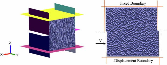
Displays the direct shear test model established for parameter calibration.
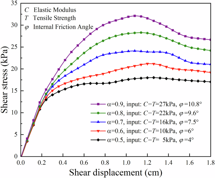
Subsequently, a series of simulations were simulated with different micro-parameters (Fig. 13a). When the parameters shown in Table 6 are used, the simulation result is similar to the laboratory test. The whole process of shearing was simulated at different pressures (50 kPa,100 kPa, 150 kPa and 200 kPa) using this set of parameters (Fig. 13b, c). The fitted results of cohesion and internal friction angle are 29.65 kPa and 12.3°, close to the parameters listed in Table 5. The corresponding micro-parameters are considered in following simulations.
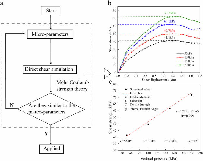
a Parameter calibration process. b Shear displacement – Shear stress under different pressures. c Fitted Line of shear strength formula. a The parameter calibration process used in the 3D direct shear test to match the laboratory data. b Displays the parameter calibration process under different vertical pressures. c Fitted line of the shear strength formula used for calibration, with data points representing experimental results.
Landslide initiation conditions
The shear strength of clays and fill soils decreases because of groundwater and rainfall. If the slope fails due to long-term creep, the landslide mass will have low water content and low fluidity. On the other hand, if there is a heavy rainfall, the fluidity of the landslide mass will significantly increase53. For clays, the shear strength can be reduced by about 50% with an increase in humidity54. In this work, the landslide is triggered by reducing the cohesion, tensile strength and friction angle of soil36. A reduction coefficient (alpha) is introduced, with values as 0.9 (extremely low water content), 0.8 (low water content), 0.7 (medium water content), 0.6 (high water content) and 0.5(high water content). The shear strength of the soil varies under different water content, so the value of α is adjusted based on the shear strength of soil. In practical applications, the shear strength of the sliding mass can be assessed by field sampling during the deformation acceleration stage. The specific value of (alpha) can be taken as the ratio of the shear strength of the sampled soil to the shear strength of the dry soil. When field experiments are unavailable, (alpha) can be calculated using pre-established water content-shear strength relationship. The water content can be obtained through monitoring or estimated using empirical curves relating rainfall and changes in the water content of the sliding mass. The mechanical properties of the landslide mass are:
where ({sigma }_{0}) and ({sigma }_{1}) are the initial and reduced tensile strengths, ({c}_{0}) and ({c}_{1}) are the initial and reduced cohesions, ({varphi }_{0}) and ({varphi }_{1}) are the initial and reduced internal friction angle, respectively, with (alpha) as the reduction coefficient. To ensure that the particle properties accurately reflect the cementation characteristics between soils, we have calibrated the micro-parameters of particles by adjusting the input values of cohesion and tensile strength. Figure 14 depicts the direct shear results of various parameters under vertical pressure of 30 kPa. Considering the particle flow method, the viscous damping changes linearly with the shear strain according to a large number of ring shear tests by Ishibashi55. The initial damping is taken to be 0.06, the end damping is taken to be 0.12.
Shows macroscopic behavior of particles with different fluidity at a vertical pressure of 30 kPa, ensuring accurate simulation of soil cementation.
Influenced by the fluidity of the sliding body, both the energy changes and accumulation morphology of the landslide would vary significantly. With the increasing of landslide fluidity ((alpha) changes from 0.9 to 0.5), the maximum average velocity of particles increases from 3.15 m/s to 4.92 m/s. The maximum kinetic energy of the sliding body increased from 1.13 × 10¹⁰J to 2.85 × 10¹⁰J showing a polynomial relationship see Fig. 15a. As (alpha) decreased, the length of landslide deposit rose from 757 m to 936 m, and the width from 539 m to 722 m, see Fig. 15b, where the width and length of the landslide are marked in Fig. 16. Figure 16 also shows the shapes of landslide with different (alpha).
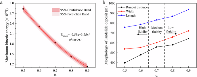
a Maximum Kinetic Energy. b Morphology of landslide deposit. a Shows the maximum kinetic energy of the sliding mass under different fluidities, analyzing the relationship between maximum kinetic energy and fluidity. b Shows the length, width, and maximum run-out of the landslide deposit morphology under different fluidities, analyzing the relationship between deposit morphology and fluidity.
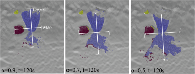
Shows the morphology of the landslide deposit under different fluidities.
Dynamic process of the landslide and influencing areas
Figure 17 shows the particle velocities of the seven monitoring points, indicating most particles tend to stop moving after 120 s. Hence this time is taken as the duration of the landslide, which can be divided into three stages:
-
1.
Initial sliding phase: 0-5 s, the sliding surface extend to the surface, and the landslide starts. The particles slide down as a whole along the sliding surface, but accumulate at the shear outlet for a short time due to the blockage of the shear outlet, see Fig. 18a.
-
2.
Steady acceleration phase: 5-15 s, the particles at the front edge of the landslide mass break through the shear outlet and rapidly spreading around. The middle and rear particles accelerate along the path of the front particles, see Fig. 18b.
-
3.
Deceleration and accumulation phase: 15-120 s, the velocity of the particles in the middle and the rear of the landslide mass rapidly decreases after reaching their maximum velocity. The front edge particles encounter less resistance, and experiencing a secondary acceleration phase after 40 s. Approximately about 80 s, the velocity of the particles in the rear tends to be 0, which accumulates near the shear outlet. However, the middle particles surge forward, breaching the shear outlet. The front edge and middle particles continue to move along the ground until the velocity decreases to 0, ultimately forming a deposit with a width of 602.9 m and length of 831. 6 m, see Fig. 18c–f.
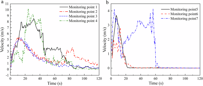
a Velocity of monitoring point 1–4. b Velocity of monitoring point 5–7. a, b Displays the motion velocity at different monitoring points on the medium fluidity, analyzing the whole sliding process.
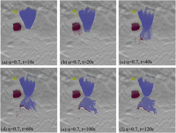
a–f Dynamic process of the lanslide morphology. a–f Shows the landslide morphology at several scenarios, visually representing the sliding process.
The total work of the landslide done by gravity is 3.2 × 10¹¹J and the ratio of kinetic energy to gravitational potential energy is 5.8%, see Fig. 19a. The majority of the gravitational potential energy is dissipated as frictional and damping energy. At around 15 s, the average velocity of all particles reaches its maximum value as 3.94 m/s when the kinetic energy reaches its maximum value as 1.85 × 10¹⁰J, see Fig. 19b. It can be found that the total kinetic energy keeps above 1010J in the first 40 s, indicating great destructive potential of the landslide. When comparing the numerical results and the aerial photo of the region, it can be found that some surrounding factories and houses are in the influencing domain, see Fig. 20. Moreover, the road could be blocked by the landslide deposits. These results offer helpful assessments for engineers who are responsible for designing warning system and slope protection.
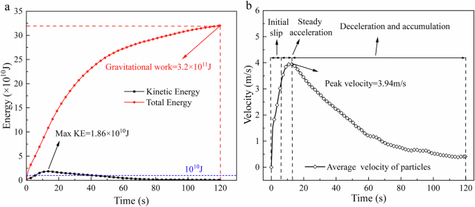
a Energy trajectory line of the landslide. b Average velocity of particles. a, b Shows the landslide’s energy trajectory line and average particle velocity, analyzing energy dissipation and landslide motion.
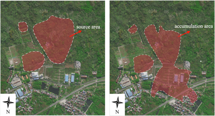
Maps the landslide’s accumulation area onto the actual map, visually representing the influencing areas.
Discussion
Based on the stability analysis presented in Section “Stability analysis and damage zones”, the safety factor of Zhutou slope is 1.24, which is lower than the stability value of 1.35 stipulated in “The technical code for building slope engineering (GB50330-2013)”. This indicates that the slope is in an unstable state and is prone to landslide under heavy rainfall or long-term wet conditions. To elucidate the interaction between groundwater seepage and soil strength, we integrated an unsaturated soil model into the seepage analysis. When the stable groundwater level during the rainy season is applied, the increase in the degree of saturation of the fill and clay layers has a significant impact on the stability of the slope. As the saturation increases, the soil strength decreases, forming a typical pre-landslide deformation pattern. This reveals the sliding mechanism of Zhutou slope, under the action of heavy rainfall, the groundwater table rises, resulting in the softening of the weak layer in the formation. This process is consistent with the landslide mechanism of slopes where most of the soil in the slip zone is clay56,57,58,59. Therefore, when conducting a risk assessment in this area, the long-term impacts of rainfall and groundwater fluctuations on the soil must be considered. Moreover, when it comes to the treatment of Zhutou slope, the primary focus of prevention and treatment should be on drainage control, including the implementation of drainage systems, water-blocking, water-diversion, and water-interception strategies.
By combining the strength reduction method with the analysis of damaged blocks, the volume of potential landslide is estimated to be approximately 2 million cubic meters. Additionally, the dynamic process of the landslide and its potential impact zones were simulated using the particle flow method. The analysis shows that the fluidity of landslide mass plays a critical role in determining the extent of the landslide. Results from the particle flow simulation indicate a polynomial relationship between landslide energy and fluidity. When the humidity increases, the kinetic energy of the landslide increases significantly, and the potential influencing areas of the landslide also expand. This suggests that in practical engineering, especially in the rainy season, it is essential to monitor changes in the fluidity of the landslide mass to predict potential failures in advance.
The three-stage process of the landslide with medium fluidity is also described in detail, including the initial sliding phase, the steady acceleration phase and the deceleration and accumulation phase. Research findings show that the sliding process is characterized by large displacement and velocity of the front particles, which indicates that the particle movement is effectively controlled by the front particles60,61. The main landslide event lasts approximately 120 seconds, releasing 3.2 × 10¹¹ J of energy, most of which is dissipated through friction and damping. The landslide has the potential to damage nearby structures and block transportation routes, highlighting the urgent need for proactive mitigation measures to prevent future disasters.
However, there are still some limitations in the simulation process. First, the 3D geological model of the Zhutou slope did not account for the effects of existing reinforcement measures, such as anti-slide piles and retaining walls. Consequently, the volume of the potential sliding mass has been overestimated. In practical engineering, the reinforcement measures will change the stress distribution within the slope and the shape of the potential sliding body. Therefore, future research should incorporate these reinforcement measures to achieve a more accurate assessment of slope stability. Additionally, real-world landslides often exhibit localized deformations and distinct failure stages, whereas our simulation results showed simultaneous deformation across three hazardous areas. Although the unsaturated soil model spatially differentiated soil parameters and revealed the weak interlayer in our simulation, it does not fully account for the complexity of material heterogeneity and existing cracks, which are critical in governing actual slope failures. The strength reduction method assumes that the entire slope is subjected to the same level of stress and weakening at the same time, which cannot fully capture the progressive failure mechanisms. To better reflect the actual landslide behavior, fully coupled hydro-mechanical models can be used to simulate the initiation and propagation of failure processes, and time-dependent effects can be considered.
In conclusion, this study assessed the stability and potential impact regions of the deforming slop using the Continuum-Discontinuum Element Method (CDEM) through a 3D numerical model based on geological observations. By integrating the unsaturated soil model into the seepage analysis and using the strength reduction method, the instability mechanism of the slope was revealed and the shape of potential slide mass was obtained. Additionally, the particle flow method was applied to simulate the landslide process, with parameters calibrated through direct shear experiments. By considering different fluidity of the landslide mass, the landslide process was analyzed by examining the total kinetic energy and average velocity of particles. Although this study provides valuable quantitative analysis for the landslide evaluation of Zhutou slope, there are still some limitations. Future research should consider the effects of the existing reinforcement measures and time-dependent effects. Overall, this study offers new perspectives and methods for slope stability analysis and landslide risk management.
: spatial distribution characteristics and implication for the seismogenic fault")

")

Responses