Crop-specific embodied greenhouse gas emissions inventory for 28 staple crops in China from 2007 to 2017

Background & Summary
Rapid economic development and population expansion have forced China to feeds 19.1% of world’s population with only 8.6% of global arable land1. To ensure food security, the production patterns of China’s agriculture become increasingly intensified and generating substantial greenhouse gas (GHG) emissions2. China’s agricultural sector, growing at an annual rate of 5%, contributes approximately 15% of national GHG emissions and accounts for 13.6% of global agricultural GHG emissions3,4,5. More importantly, agriculture represents a major sources of methane (CH4) and nitrous oxide (N2O) emissions, responsible for 41.79% and 65.44%, respectively, to the national totals of these GHGs6. In 2020, China has pledged to achieve carbon neutrality before 2060 in a way that effectively reduces GHG emissions7. To achieve this goal, it is necessary to conduct a comprehensive assessment of agricultural GHG emissions to identify mitigation opportunities.
As a crucial component of China’s agricultural output, crop farming emitted close to 60% of China’s agricultural GHG emissions and emerged as the focus of national GHG reduction agenda5,8. Different from other agricultural production sectors, crop farming not only directly generate a large amount of GHG emissions (e.g., CH4 emissions from rice cultivation and N2O emissions from synthetic fertilizer application), but the consumption of agricultural inputs (e.g., synthetic fertilizers, pesticides and plastic film) also indirectly drive a great deal of GHG emissions from the industrial and energy industries9. At present, the over-reliance on the consumption of agricultural inputs to enhance crop yield has become the main features of China’s crop farming10,11. This over-reliance has promoted the agricultural inputs of synthetic fertilizers, pesticides and plastic film growth rapidly with an annual rate of 3.07%, 3.06%, and 6.33%, respectively, from 1990 to 201712,13. To achieve effective mitigation policy-making, it is necessary to have a comprehensive understanding of the embodied GHG emissions, encompassing both direct and indirect GHG emissions, in China’s crop farming.
Thus far, in China, most related studies have quantified the embodied GHG emissions at the entire crop farming system level14,15,16. However, a holistic and systematic embodied GHG emission inventory for crop-specific level is still lacking. In fact, there was significant heterogeneity in the emissions status and structures across different crop types17,18. Clarifying the emissions status and structure at crop-specific level has important guiding significance for formulating more accurate emission mitigation strategies1. To this end, Cheng et al.17 and Xia et al.19 calculated the embodied GHG emissions for China’s four staple crops (rice, wheat, maize and soybean). Building upon this, Lin et al.20 systematically measured the embodied GHG emissions from China’s three major grain crops (rice, wheat and maize) and six hybrid grain groups. Further expanding the scope, Xu and Lan21 and Zhen et al.22 assessed the embodied GHG emissions of 24 and 32 China’s staple crops, respectively.
In general, there are three main deficiencies in existing studies that focus on crop-specific embodied GHG emissions in China. First, previous studies predominantly focus on quantifying the embodied GHG emissions of major grain crops (rice, wheat and maize) at the national level, information on embodied GHG emission status and structure of other staple crops at China’s provincial level is still lacking. Since there are significant difference exists in production modes across provinces and crop types in China, inducing obvious heterogeneity in crop-specific embodied GHG emissions for various crop types across diverse provinces1,23. Hence, it is necessary to systematically measure embodied GHG emissions for various crop types across diverse provinces, so as to provide support for clarifying the emission mitigation priorities of China’s crop farming. Second, previous studies usually employed national uniform emission factors to measure provincial crop-specific embodied GHG emissions, disregarding provincial-specific nuances in the production processes of agricultural inputs. This makes it easy for the embodied GHG emissions of the same crop type to be overestimated or underestimated across provinces, leading to misguided emission mitigation strategies24. Third, previous studies primarily focus on the magnitude of crop-specific embodied GHG emissions per unit area or yield, offering limited information for mitigation decision-making. The crop-specific embodied GHG emissions per unit yield can help policymakers to identify the cost-effective measures to decouple yields from GHG emissions25,26. While assessing the specific mitigation effects of these measures requires considering the dynamic changes in crop-specific embodied GHG emissions per unit area27,28. Therefore, crafting the most economical and effective emission mitigation measures necessitates a comprehensive understanding that integrates both yield- and area-based crop-specific emission data.
Addressing the aforementioned limitations, this study builds a provincial crop-specific embodied GHG emission inventory for 28 staple crops in China across five years (2007, 2010, 2012, 2015 and 2017). Employing a hybrid environmentally extended multi-regional input-output and life cycle assessment (EEMRIO-LCA) model, this study quantified both direct and indirect GHG emissions per unit area and yield for various crop types across diverse provinces. This investigation offers the most comprehensive and detailed dataset of its kind in China. By clarify the status and structure of crop-specific embodied GHG emissions per unit area and yield across provinces, this study sheds light on empowers stakeholders to formulate more targeted and effective emission mitigation strategies for China’s crop farming.
Methodology and Data Source
In this study, the crop-specific embodied GHG emissions per unit area and yield in China were calculated by using a hybrid EEMRIO-LCA model. The crop-specific embodied GHG emission is composed by direct and indirect components20. Among them, the direct GHG emissions refer to CH4 emissions from rice cultivation, N2O emissions from synthetic fertilizer application, GHG emissions from diesel oil used on farms and electricity used for irrigation22. The indirect GHG emissions denote the GHG emissions caused by the off-farm production processes of agricultural production inputs, such as seeds, synthetic fertilizers, pesticides, and agricultural machinery29. The direct GHG emissions can be measured using a bottom-up based process analysis, while the indirect GHG emissions can be captured through a top-down EEMRIO analysis20,30. Figure 1 describes the accounting framework of crop-specific embodied GHG emissions in China.

The accounting framework of crop-specific embodied GHG emissions.
Leveraging the established accounting framework, this study compiled the crop-specific embodied GHG emission inventories covered 28 staple crops across 30 Chinese provinces (excluding Tibet Autonomous Region, Hong Kong and Macao Special Administrative Region, and Taiwan province) for the years 2007, 2010, 2012, 2015 and 2017. The 28 staple crops encompass seven grain crops and 21 cash crops. Table 1 detailed the classification of these staple crops. These 28 staple crops are highly representative for China’s crop farming, representing 82.9% of the national total sown area and 92.4% of total crop yield in 201731. In the following calculations of crop-specific embodied GHG emissions, all types of GHGs, including CO2, CH4 and N2O, were converted into CO2 equivalent emissions. In this case, the Global Warming Potential (GWP) parameters for the 100-year time horizon published by IPCC32 were adopt to converted CH4 (GWP100 = 25) and N2O (GWP100 = 298) emissions into CO2 equivalent emissions.
Direct GHG emission calculation
According to Lin et al.20 and Dong et al.33, crop-specific direct GHG emissions can be quantified through a bottom-up based process analysis as follows:
where ({G}_{i,j}^{D}) denotes the areal direct GHG emissions of crop type i in province j; ({G}_{i,j,a}^{D}) represents the areal direct GHG emissions of crop type i in province j from activity a; ({V}_{i,j,a}^{D}) refers to the areal amount of activity a for crop type i in province j; and (E{F}_{i,j,a}) is the GHG emission coefficient of activity a in province j.
The data on crop-specific areal application rates of synthetic fertilizers, costs for diesel oil used on farms, and electricity charges for irrigation were collected from the China Agricultural Products Cost-Benefits Yearbooks34,35,36,37,38. The N2O emissions from synthetic fertilizer application mainly generated from the application of N fertilizers and compound fertilizers. Consistent with Wang et al.39, a 30% N fraction was set for compound fertilizers. As the China Agricultural Products Cost-Benefits Yearbooks only provide the crop-specific areal costs for diesel oil used on farms. Thus, the provincial diesel oil prices were collected from website (https://data.eastmoney.com) to calculate crop-specific areal diesel oil consumption amount. The provincial CH4 emission coefficients of rice cultivation and provincial N2O emissions from synthetic fertilizer application were drawn from the Guidelines for the Preparation of Provincial Greenhouse Gas Inventories40. The GHG emission coefficients of diesel oil were sourced from Liu et al.23 and Shan et al.41. All these data collection were followed a double-validation approach, with one member of our group collected data and then confirmed by another member42,43. It worth noting that although the GHG emissions from electricity used for irrigation is classified as the direct GHG emissions, while the GHG emission coefficients of electricity were determined by using the EEMRIO analysis to capture the full environmental impact during its production process, as suggested by Zhen et al.22 and Long et al.44.
Indirect GHG emission calculation
Referring to Reynolds et al.30 and Acquaye et al.45, crop-specific indirect GHG emissions can be captured using a top-down based EEMRIO analysis. Suppose there are m regions in China, and each region contains n economic sectors. By using the EEMRIO analysis, the embodied GHG emission intensities of agricultural inputs, i.e., the GHG emissions from the production of agricultural inputs can be expressed as follows:
where e denotes a 1 × mn sectoral embodied GHG emission intensity vector, with the element ({{e}}_{j,b}(bin n,{j}in {m})) represents the embodied GHG emission intensity for sector b in province j, i.e., the embodied GHG emission intensity of agricultural input b in province j; f refers to a 1 × mn sectoral direct GHG emission intensity vector; I is an mn × mn identity matrix; A denotes a mn × mn intermediate input matrix; and ({({bf{I}}-{bf{A}})}^{-{bf{1}}}) represents a mn × mn Leontief inverse matrix.
Based on the calculated embodied GHG emission intensities, the crop-specific indirect GHG emissions can be measured as follows:
where ({G}_{i,j}^{I}) denotes the areal indirect GHG emissions of crop type i in province j; ({G}_{i,j,b}^{I}) represents the areal indirect GHG emissions of crop type i in province j from agricultural production input b; and ({V}_{i,j,b}^{I}) refers to the areal cost of agricultural production input b for crop type i in province j.
The calculation of crop-specific areal indirect GHG emissions called for the data on: Chinese MRIO tables, sectoral primary energy consumption, GHG emission coefficients of different energy types, and crop-specific areal costs of different agricultural inputs. The Chinese MRIO tables for 2007 (contains 30 regions and 30 economic sectors), 2010 (contains 30 regions and 30 economic sectors), and 2012 (contains 31 regions and 42 economic sectors) were obtained from Liu et al.46,47,48. The Chinese MRIO tables for 2015 (contains 31 regions and 42 economic sectors) and 2017 (contains 31 regions and 42 economic sectors) were taken from Zheng et al.49. Due to inconsistencies in the classification of regions and economic sectors, we harmonized all tables into a consistent format with 30 regions and 30 economic sectors. Table S1 shows the detailed sectoral information.
Data on provincial primary energy consumption for each economic sector were collected from China’s Emission Accounts Datasets (CEADs)50,51, encompassing 47 economic sectors and 17 energy types. Since the number of economic sector for primary energy consumption data are inconsistent with the harmonized Chinese MRIO tables. We aggregated the economic sectors of provincial primary energy consumption data to match with the harmonized Chinese MRIO tables. The updated GHG emission coefficients for each energy types were extracted from Shan et al.41, Xu et al.52 and Liu et al.53. In addition, data on crop-specific areal costs for various agricultural inputs were obtained from the China Agricultural Products Cost-Benefits Yearbooks34,35,36,37,38. As with direct GHG emission calculations, data collection followed a double-validation approach, with one group member extracting dada and another verifying it.
Crop-specific embodied GHG emission calculation
In this study, both the metrics of crop-specific embodied GHG emissions per unit area and per unit yield were used to comprehensively uncover the impact of different staple crops on global climate change. The crop-specific embodied GHG emissions per unit area can be calculated as follows:
where ({G}_{i,j}^{Area}) denotes the crop-specific embodied GHG emissions per unit area of crop type i in province j.
Based on the calculation of crop-specific embodied GHG emissions per unit area, the crop-specific embodied GHG emissions per unit yield can be measured as:
where ({G}_{i,j}^{Yield}) denotes the crop-specific embodied GHG emissions per unit yield of crop type i in province j; DMi,j refers to the dry matter yield per unit area of crop type i in province j.
The data on provincial areal yield and dry matter content factors for various staple crops are essential for crop-specific embodied GHG emission calculation. The provincial areal yield of different staple crops were collected from the China Agricultural Products Cost-Benefits Yearbooks34,35,36,37,38. The dry matter content factors which used to convert provincial areal yield of different staple crops into dry matter were obtained from Piao et al.54 and Zhu et al.55. Consistent with the calculations for direct and indirect GHG emissions, a double-validation approach was employed. One of our group member extracted and calculated the crop-specific embodied GHG emissions, while another member independently verified the results.
Data Records
All the data were compiled in an Excel workbook named as “China’s crop-specific embodied GHG emission inventory” that consists of 3 data sheets, uploaded on Figshare56.
-
(1)
GHG per unit area (or yield) is a sheet that summarized the crop-specific embodied GHG emission per unit area and yield for 28 staple crops of 30 Chinese provinces across years 2007, 2010, 2012, 2015 and 2017. Each entry in the sheet details:
-
Specific classification information of 28 staple crops, including Category (column A), Subcategory (column B), and Crop type (column C).
-
The data collection context, including Year (column D), and Region (column E) of data origin.
-
The crop-specific embodied GHG emissions, including Crop-specific embodied GHG emissions per unit area (represents by the crop-specific embodied GHG emissions per hectare in column F), and Crop-specific embodied GHG emissions per unit yield (represents by the crop-specific embodied GHG emissions per unit dry matter yield in column G).
-
(2)
GHG structures per unit area/yield sheet reports the compositions of crop-specific embodied GHG emissions per unit area and yield, respectively. Similar to the previous sheet, it provides the following information for each staple crops:
-
Specific classification information of 28 staple crops, including Category (column A), Subcategory (column B), and Crop type (column C).
-
The data collection context, including Year (column D), and Region (column E) of data origin.
-
The compositions of crop-specific direct GHG emissions per unit area/yield, including CH4 emissions from rice cultivation (column F), N2O emissions from synthetic fertilizer application (column G), GHG emissions from diesel oil used on farms (column H), and GHG emissions from electricity used for irrigation (column I).
-
The compositions of crop-specific indirect GHG emissions per unit area/yield, including GHG emissions from the production of seeds (column J), synthetic fertilizers (column K), pesticides (column L), plastic film (column M), agricultural machinery (column N), trellis and small farm implements (column O).
-
The aggregate values of direct and indirect GHG emissions, i.e., Crop-specific embodied GHG emissions per unit area/yield (column P), combining both direct and indirect GHG emissions.
Figure 2 illustrates the temporal trends of average embodied GHG emissions for 28 staple crops at the national level between 2007 and 2017. The analysis reveals that grain crops exhibited higher embodied GHG emissions per unit area compared to cash crops, while cash crops demonstrated greater embodied GHG emissions per unit yield. Over the study period, 17 out of the 28 staple crops showed a decrease in their per-area embodied GHG emissions, and 20 crops experienced reduced per-yield embodied GHG emissions.
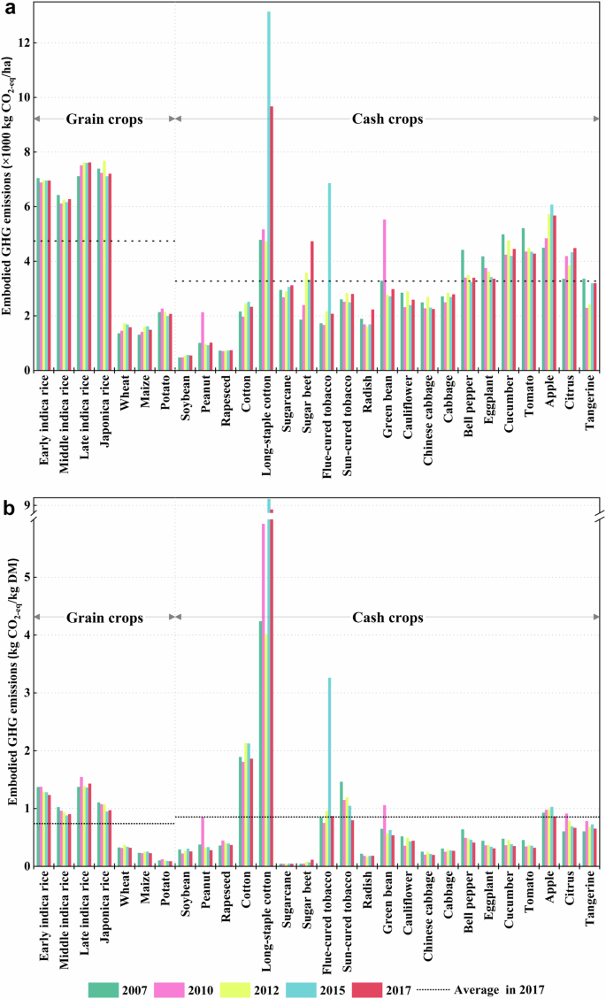
Trends in crop-specific national average embodied GHG emissions during 2007–2017. (a) The crop-specific average embodied GHG emissions per unit area; (b) The crop-specific average embodied GHG emissions per unit yield).
Figure 3 provides a detailed analysis of the embodied GHG emission structures across 28 staple crops at the national level in 2017. For grain crops, rice cultivation emerged as the primary emission source, accounting for 68.41% and 71.49% of emissions per unit area and yield, respectively, followed by synthetic fertilizer application (12.60% and 12.42%). In contrast, cash crops showed different emission patterns, with irrigation-related electricity consumption being the dominant source (28.92% per unit area and 39.39% per unit yield), followed by synthetic fertilizer application (24.56% and 18.30% for area and yield metrics, respectively).
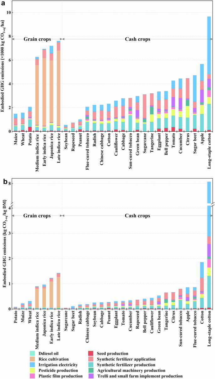
Structures of crop-specific national average embodied GHG emissions in 2017. (a) The crop-specific average embodied GHG emissions per unit area; (b) The crop-specific average embodied GHG emissions per unit yield).
Technical Validation
Uncertainty analysis
Based on the calculation method employed, the uncertainty of our crop-specific embodied GHG emissions dataset mainly arises from the following five aspects.
-
(1)
Crop-specific activity data. The crop-specific activity data used in this study, including crop-specific areal application rate of synthetic fertilizers, areal electricity charges for irrigation, and areal costs for diesel oil and other agricultural inputs used on farms. All these crop-specific activity data were droved from the statistical yearbooks published by the government official, which were identified as little or relatively low level of uncertainty16,24. Hence, the uncertainty of crop-specific activity data was not quantified in this study.
-
(2)
GHG emission coefficient. The GHG emission coefficients used to calculate crop-specific embodied GHG emissions encompassed the provincial CH4 emission coefficient for rice cultivation, provincial N2O emission coefficient for synthetic fertilizer application, and the GHG emission coefficients for various energy types. The coefficients of variations (CV) for provincial CH4 emission coefficient of rice cultivation were derived from Liang et al.16 and Yan et al.57, as shown in Table S2. The ranges of distribution for provincial N2O emission coefficient of synthetic fertilizer application were drawn from the Guidelines for the Preparation of Provincial Greenhouse Gas Inventories40, presented in Table S3. The CVs for GHG emission coefficients of various energy types were collected from existing studies. The CVs for CO2 emission coefficients of various energy types were taken from Shan et al.50, while the CVs for CH4 and N2O emission coefficients of various energy types were extracted from Liang et al.16 and Zhao et al.58. All these parameters were shown in Table S4.
-
(3)
Sectoral primary energy consumption data. In this study, the provincial primary energy consumption data for each economic sector compiled by CEADs were used to calculate the embodied GHG intensities of different agricultural inputs. The CEADs also reports the CVs of primary energy consumption data for various economic sectors50,59, as shown in Table S5.
-
(4)
Chinese MRIO table. The calculation of crop-specific indirect GHG emissions was based on the Chinese MRIO tables. However, quantifying the uncertainty of these tables is challenging, as the uncertainty information is rarely reported in the literatures. Therefore, following Wei et al.43 we adopted the CVs of input-output coefficients (ranging from 1%–50%) provided by Hertwich and Petters60 as the proxy data to quantify the uncertainty of Chinese MRIO tables.
-
(5)
Crop-specific dry matter content factor. The crop-specific dry matter content factors were essential for compiling the inventory of crop-specific embodied GHG emissions per unit yield. However, these factors are also rarely reported in existing studies, resulting in the detailed uncertainties of crop-specific dry matter content factors remaining uncaptured. Therefore, following the study of Yu and Tan24, the CVs of crop-specific dry matter content factors were set at 15%, as the unofficially published crop-specific dry matter content factors were used in this study.
Monte Carlo simulations were employed to quantify the combined uncertainty of the crop-specific embodied GHG emission inventory. Based on the CVs of the above source data, we conducted 50,000 Monte Carlo simulations for above source data, and the estimations of 95% confidence interval were used. The 95% confidence intervals of crop-specific national average embodied GHG emissions in 2017 are shown in Fig. 4. The detailed uncertainty results for crop-specific embodied GHG emission inventory in 2017 are shown in Tables S6 and S7. For crop-specific embodied GHG emissions per unit area (Fig. 4a), rapeseed had the highest uncertainty (−39.00%~46.81%), while late indica rice had the lowest uncertainty (−26.69%~17.84%) in 2017. In contrast, crop-specific embodied GHG emissions per unit yield exhibited relatively lower uncertainties (Fig. 4b). In 2017, the uncertainty of rapeseed’s embodied GHG emissions per unit yield also turns to be the highest (−33.86%~36.71%), while the embodied GHG emissions per unit yield of late indica rice exhibited the lowest uncertainty (−20.34%~10.07%).
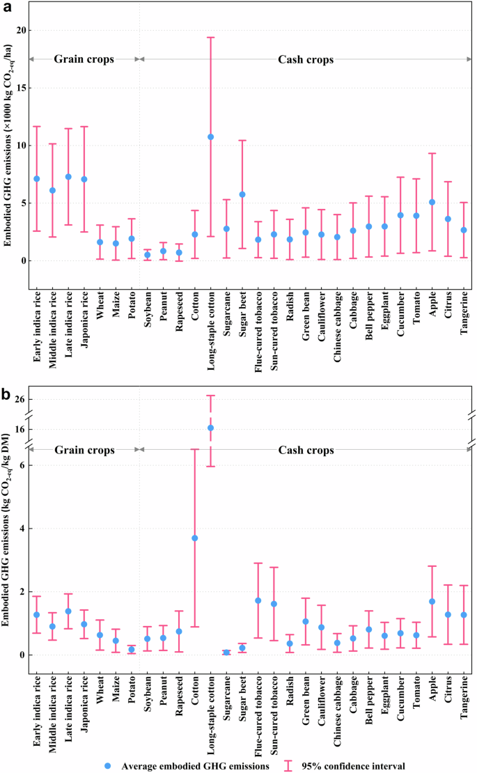
Uncertainties of crop-specific national average embodied GHG emissions in 2017. (a) The crop-specific average embodied GHG emissions per unit area; (b) The crop-specific average embodied GHG emissions per unit yield).
Comparison with existing studies
Since the uncertainty analysis does not play a decisive role in the truth values of this study24, we further validated our datasets by comparing our results with existing studies that adopted the LCA17,19,21. We compared our results with these studies at the national level, as only national level datasets are available in these studies. Cheng et al.17 and Xia et al.19 have reported the crop-specific GHG emissions per unit yield for China’s three major grain crops (rice, wheat and maize) and one oil crops (soybean) in 2011 and 2010, respectively. Hence, we compared the crop-specific embodied GHG emissions per unit yield in 2010 of our study with their results (Fig. 5a). Xu and Lan21 reported the crop-specific GHG emissions per unit yield for China’s 21 staple crops (including 4 grain crops and 17 cash crops) in 2013. Consequently, we compared the crop-specific embodied GHG emissions per unit yield in 2012 with their results (Fig. 5b).
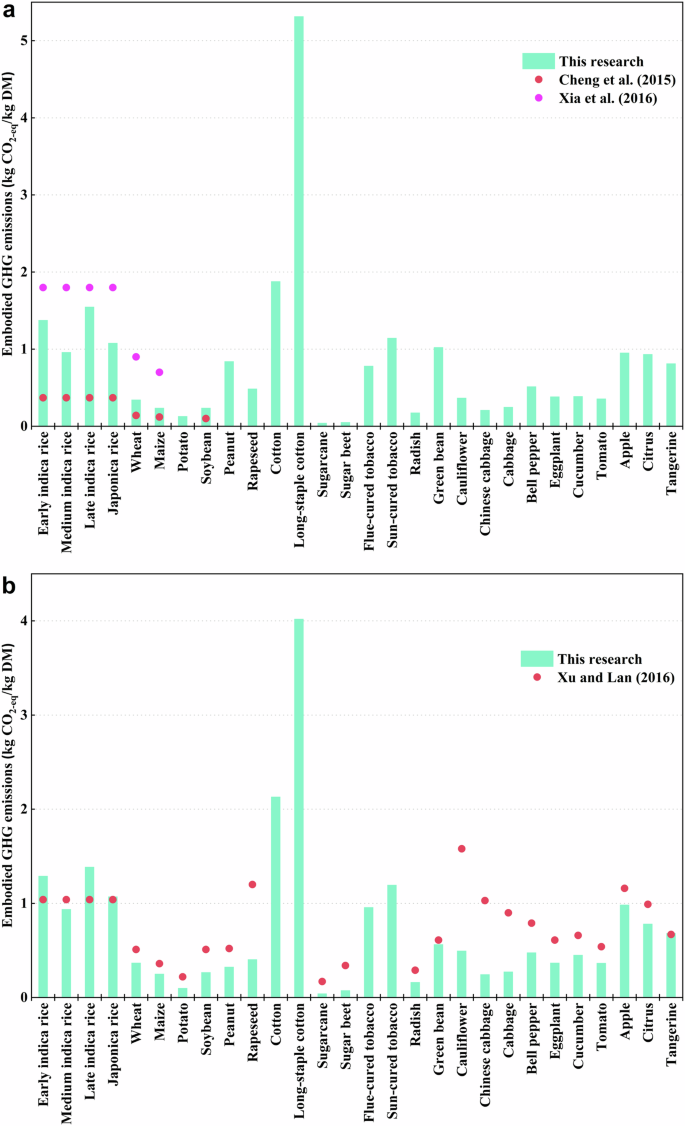
Comparison of crop-specific national average embodied GHG emissions per unit yield in this research with other studies. (a) Comparison of crop-specific average embodied GHG emissions per unit yield in 2010; (b) Comparison of crop-specific average embodied GHG emissions per unit yield in 2012).
Generally, the crop-specific embodied GHG emissions per unit yield measured in our study higher than the estimation of Cheng et al.17, but lower than those of Xia et al.19 and Xu and Lan21. The reasons for this difference can be summarized in two aspects. On the one hand, there were differences in the boundary of the accounting framework. For example, the GHG emissions from the production of seeds, agricultural machinery, trellis and small farm implements, which are primarily provided by emission-intensive industries and occupy a considerable proportion in the emission structures across staple crops (Fig. 3b)11,53, were not included in the accounting framework of Cheng et al.17. As a result, the crop-specific GHG emissions were inevitably grossly underestimated.
On the other hand, there were differences in the embodied GHG emission intensities of agricultural inputs. The present study applied EEMRIO analysis to capture the provincial-specific embodied GHG emission intensities for different agricultural inputs. This approach can captures the GHG emissions of the entire supply chains during the production processes of various agricultural inputs, avoiding the truncation error inherent in LCA30,61. More importantly, this approach fully reflects the difference of provincial production technology level and prevents the embodied GHG emission intensity of various agricultural inputs from being overestimated45,62. For instance, both Xia et al.19 and Xu and Lan21 extracted a national uniform GHG emission intensity for the production of pesticides from existing studies. However, compared to present study, this nationally uniform GHG emission intensity resulted in an overestimation of GHG emissions from the production of pesticides by 29.62% to 90.74% across Chinese provinces. This means that setting GHG emission intensity based on existing studies not only fails to reflect the differences in the production technology of agricultural inputs across Chinese provinces, but also result in a serious underestimation of crop-specific embodied GHG emissions.
Limitations
This study is subject to two primary limitations. First, our crop-specific embodied GHG emissions inventory is constrained to five specific years (2007, 2010, 2012, 2015, and 2017) due to the limited availability of Chinese MRIO tables. Second, while this study compiles a provincial crop-specific embodied GHG emission inventory for 28 staple crops in China, we present only national average results to ensure data consistency and contain the study’s scope. Future research could build on this inventory to examine temporal trends in embodied GHG emissions at the provincial level, providing deeper insights into regional variations and characteristics.

Responses