Data-efficient construction of high-fidelity graph deep learning interatomic potentials

Atomistic simulations are an essential tool in materials science. A key input to atomistic simulations is an interatomic potential (IP) or force field that describes the potential energy surface (PES). Over the past decade, machine learning (ML) has emerged as a powerful approach to constructing IPs^1,2,3 by learning the PES from a dataset of reference quantum mechanics (QM) calculations^{4,5,6,7,8,9,10}. Such machine learning potentials (MLPs) typically achieve remarkably improved accuracies in terms of energy and force errors over traditional empirical IPs¹¹ and can be fitted more readily to more complex chemistries^12,13. MLPs have enabled studies inaccessible to either QM or empirical IPs, including the study of short-range chemical order and dislocation motion in high-entropy alloys^14,15,16, long-time scale diffusion in lithium superionic conductors^17,18,19, etc. More recently, a new class of MLPs based on graph deep learning (GLPs) has been developed^20,21,22,23. GLPs utilize a natural graph representation for a collection of atoms, where the atoms are the nodes and the bonds between them are the edges. The information then passes through the graph via a series of message-passing steps, typically modeled using neural networks. The primary advantage of GLPs is their ability to handle arbitrary complex chemistries, without combinatorial explosion in the feature space associated with local environment-based MLPs²⁴. Indeed, universal MLPs with coverage of the entire periodic table, such as the Materials 3-body Graph Network (M3GNet)²⁰, Crystal Hamiltonian Graph Network (CHGNet)²¹ and Message-passing Atomic Cluster Expansion (MACE)²², have been trained using large public datasets of QM structural relaxations from the Materials Project²⁵ and have broad applications in materials discovery and dynamic simulations.

The biggest bottleneck in MLP construction is the computation of the reference QM data set. For this reason, most MLPs today are fitted using data computed using relatively low-cost semi-local density functional theory (DFT) methods at the generalized gradient approximation (GGA) level, such as the Perdew-Burke-Ernzerhof (PBE) functional²⁶. More accurate functionals exist. For instance, the strongly constrained and appropriately normed (SCAN) functional designed to recover all 17 exact constraints presently known for meta-GGA functionals has been demonstrated to yield significantly improved geometries and energies for diverse materials²⁷. In quantum chemistry, post-Hartree Fock (post-HF) methods such as CCSD(T) can achieve chemical accuracy in energies (within 1 kcal mol⁻¹ of experiments). However, such improved accuracies generally come at a much higher computational expense and poorer scaling²⁸.

Various approaches have been developed to minimize the computational expense involved in generating training data for high fidelity (hifi) MLPs. One widely used approach is transfer learning (TL), in which a pre-trained MLP constructed using low fidelity (lofi) data, such as DFT and HF, is fine-tuned using a reduced amount of hifi data^29,30,31. TL has also been demonstrated in property prediction models^32,33,34,35. A common TL approach is to fix the embedding layers in a GNN, which is expected to improve the transferability to unseen structures and accelerate the convergence of model training. However, this can potentially reduce model accuracy due to a decrease in the number of learnable parameters. Recently, Shoghi et al.³⁶ proposed a supervised joint multi-domain pretraining scheme for transfer learning in combination with data normalization and temperature sampling to address the imbalance of dataset sizes and range of energies and forces. Such a scheme enables model training across multiple datasets spanning diverse chemical domains within a multi-task framework. Another popular approach is Δ—learning, which trains a model to reproduce the difference between the baseline and target methods^{37,38,39,40,41}. However, Δ—learning requires the same data to be present in both the baseline and target methods, which is a severe constraint for MLP development.

Uniquely among the GLP architectures developed so far, the M3GNet architecture incorporates a global state feature (Fig. 1). Previously, Chen et al.⁴² have demonstrated the use of the global state feature for fidelity embedding to train a Materials Graph Network (MEGNet) model to predict band gaps using data from multiple fidelity (mfi) sources (different functionals, experiments). The inclusion of a large quantity of low-fidelity (lofi) PBE band gaps was found to greatly enhance the resolution of latent structural features in MEGNet, which can markedly decrease the mean absolute errors (MAEs) of hifi band gap predictions by 22–45%. Most critically, this improvement in accuracy was achieved without an increase in the amount of hifi training data. Similar works based on mfi band gap prediction for metal-organic framework⁴³ and optical crystals⁴⁴, formation enthalpy of materials⁴⁵ and optical molecular peak⁴⁶ have also been reported. Compared to transfer learning or Δ − learning, the multi-fidelity approach is more flexible as it does not require a pre-trained baseline model or the same data in different fidelities.

Every structure is represented as a graph, considering atoms as nodes, bonds as edges, and the fidelity of reference methods as global state attributes. Atomic numbers and radial basis functions are embedded in latent node features and edge features, respectively. The fidelity of each data point is encoded as an integer (e.g. 0: low-fidelity, 1: high-fidelity in this work) to distinguish different levels of reference electronic structure methods. These integers are then embedded into the corresponding learnable state features. The information between nodes, edges and global state features are iteratively exchanged via sequential three-body interactions and graph convolutions. The resulting atomic features are fed into the readout layer yielding atomic energies. The summation of atomic contributions is equal to the potential energy of the system computed with the given fidelity method.

Full size image

In this work, we demonstrate the application of the mfi approach to construct highly accurate M3GNet GLPs for two model systems—silicon and water. Both silicon and water have been extensively investigated with DFT at different levels of approximations^{47,48,49,50,51,52,53}, and the reported properties can be qualitatively different depending on the reference methods. For silicon, the radial distribution function (RDF) of liquid silicon computed with the SCAN functional is in better agreement with the experimental RDF due to its clearer discrimination of metallic and covalent bonds^49,54. Furthermore, recent studies show that an MLP trained on SCAN data outperforms that trained on PBE data in terms of predictions of structural transitions from amorphous to polycrystalline phases at different external pressures⁵⁵, with a Δ − learning MLP trained on more accurate random phase approximation (RPA) calculations as a reference⁵⁶. For water, meta-GGA and hybrid functionals such as SCAN^57,58 and SCAN0⁵⁹ provide more accurate descriptions of hydrogen bonding and van der Waals interactions than GGA functionals such as revised-PBE (RPBE) and BLYP^60,61,62. We will demonstrate that with appropriate sampling, an mfi-M3GNet can be extremely efficient in terms of hifi data requirements, requiring 10% coverage of SCAN data to achieve similar accuracies as an M3GNet GLP trained on an extensive SCAN dataset. We also provide comprehensive benchmarks reproducing the structural properties of liquid water and amorphous silicon, the Murnaghan equation of state, and the relaxed geometries of crystals. These results illustrate a data-efficient pathway to the construction of hifi GLPs.

Multi-fidelity M3GNet architecture

The M3GNet architecture has already been extensively covered in our previous work, and interested readers are referred to ref. ²⁰ for details. Here, we will discuss only the modifications for the treatment of data of multiple fidelities. For brevity, we will discuss the modifications in the context of datasets comprising only two fidelities, which is the most common scenario for PES datasets; extension beyond two fidelities is trivial⁴². The fidelity information (lofi RPBE/PBE and hifi SCAN) is encoded as integers (lofi: 0 and hifi: 1) and embedded as a vector in the global state feature input to the M3GNet model (Fig. 1). This fidelity embedding encodes the complex functional relationship between different fidelities and their associated PESs and is automatically learned from the training dataset. The edges, nodes, and global state features are repeatedly updated through a series of interaction blocks that involve sequential three-body interactions and graph convolutions. The resulting atomic feature vectors, which represent the combined information of local chemical environments and fidelity, are fed into gated multi-layer perceptrons for the calculation of atomic energies.

In the following sections, we will present the benchmarks for the performance of mfi M3GNet models for silicon and water against DFT and 1fi M3GNet models. Figure 2 illustrates the selection of lofi PBE/RPBE and hifi SCAN data for training, validation and test sets for constructing 10%-mfi SCAN and 80%-1fi SCAN models. As there is large overlap in structures between the lofi and hifi SCAN datasets⁵⁵, only 80% of the lofi data combined with 10% of the hifi data selected from structures within the 80% lofi data were used to train the mfi models. The 20% of SCAN data points, where the structures did not appear in both the lofi and hifi training sets, were divided into equal validation and test sets. This process avoids the possibility of including the same structures in the training and the validation/test sets, which allows for a robust comparison of different sampling sizes and techniques.

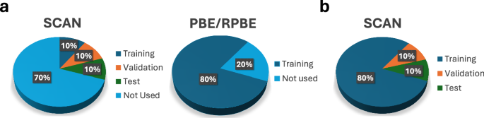
In the pie charts, similar positions correspond to similar structures. a The training set (dark blue regions) for the 10%-mfi SCAN model comprises 10% of the hifi SCAN data and 80% of the lofi PBE/RPBE data. The validation (orange region) and test (green regions) sets are constructed by splitting equally the 20% of the hifi SCAN data that do not appear in either the PBE/RPBE or SCAN training data. b For the 80%-1fi SCAN models, 80% of SCAN data were used for training. The same structures were used for validation and test sets as the mfi SCAN model.

Full size image

Silicon

In this section, we develop mfi and 1fi M3GNet IPs for silicon and benchmark their performance in reproducing not only basic energy and forces, but also structural properties of crystalline polymorphs and amorphous silicon as well as derived bulk properties such as the bulk modulus.

Convergence with percentage of hifi data points

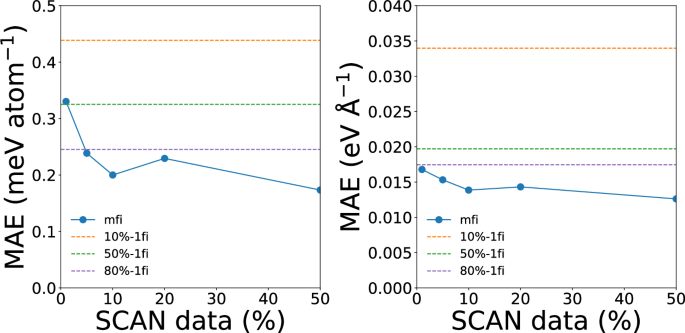
Figure 3 shows the convergence of the energy and force errors of the mfi M3GNet models for silicon with respect to the percentage of hifi (SCAN) data. Here, the Dimensionality-Reduced Encoded Cluster with Stratified (DIRECT) sampling approach developed by the current authors was used to ensure robust coverage of the configuration space regardless of the size of the SCAN dataset. With only 10% of SCAN data, the mfi M3GNet model already achieves comparable energy and force MAEs as the 1fi M3GNet potential trained on the 80% of SCAN data. Further decreases in MAEs with the increasing amount of SCAN training data are relatively small. Furthermore, we note that the MAEs of the 1fi M3GNet models are significantly higher than that of the mfi M3GNet models with comparable SCAN training data sizes. For example, the 10%-1fi M3GNet model has energy and force MAEs of 0.062 eV atom^-1 and 0.127 eV Å⁻¹, respectively, compared to the 10%-mfi M3GNet model energy and force MAEs of 0.032 eV atom^-1 and 0.100 eV Å⁻¹, respectively. Even for 50% SCAN data, the mfi model significantly outperforms the 1fi model. Hence, the inclusion of the large quantity of lofi PBE data improves the quality of hifi SCAN predictions.

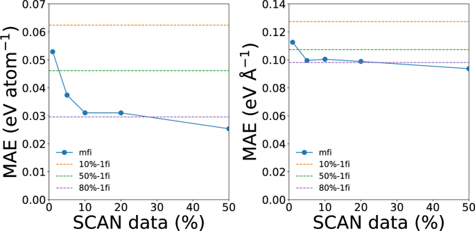
The test mean absolute errors (MAEs) of mfi M3GNet GLPs trained with different percentages of SCAN data for silicon. The dashed lines represent the MAEs of the 1fi M3GNet potential trained on 10%, 50% and 80% of SCAN data for reference.

Full size image

Effect of sampling

To explore the effect of sampling of hifi data on the performance of mfi M3GNet models, we trained 10%-mfi M3GNet models, with the 10% SCAN data sampled (a) from a narrow region (denoted as “10% mfi-narrow”), (b) in random manner (denoted as “10% mfi-random”), and (3) DIRECT sampling. The “narrow” sampling only includes primarily diamond crystal structures with distortions, strains and defects and excludes amorphous and other structures with more diverse local environments. Figure 4 illustrates the coverage of the three different sampling techniques using the first two principal components (PCs) of the encoded structure features, which were obtained using the pretrained M3GNet formation energy model as a structure featurizer.

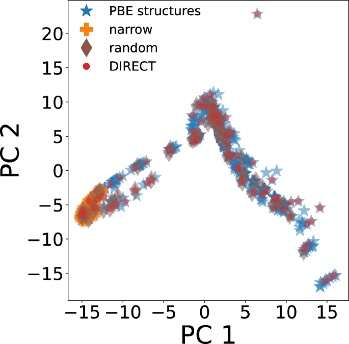
The narrow sampling approach only samples structures from the far left of the PC space. The random sampling approach significantly improves the coverage of the entire space, but structures in the extrema of the latent space are missed. Finally, DIRECT sampling ensures coverage of the entire latent space, including extreme regions such as an isolated atom and highly distorted structures.

Full size image

From Fig. 5, it can be observed that the 10%-mfi-DIRECT and 10%-mfi-random models exhibit similar test MAEs in energies and forces, but the 10%-mfi-narrow model exhibits extremely high test MAEs. These results illustrate that the 10%-mfi-narrow model extrapolates poorly beyond the training domain for the majority of the validation and test structures. This can be supported by the plot of the first two principal components of the training, validation, and test structures, as provided in Fig. S1. The validation errors, which share the same observations as the test errors, are plotted in Fig. S2. To further evaluate the accuracy of 10%-mfi-random and 10%-mfi-DIRECT, we selected 297 bulk structures with great structural diversity from GAP-18 dataset⁵⁶, which is used for constructing general-purpose IPs of silicon, to compare the error of energies and forces with respect to DFT-SCAN. The MAEs in energies and forces of 10%-mfi-random are 0.114 eV atom⁻¹ and 0.088 eV Å⁻¹, respectively, while those of the 10%-mfi-DIRECT are 0.040 eV atom⁻¹ and 0.091 eV Å⁻¹, respectively. This clearly shows that the GLP achieves better accuracy with respect to unseen structures with DIRECT sampling.

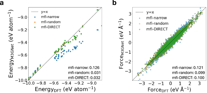
Parity plots of (a) energies and (b) forces predicted by 10%-mfi-narrow, 10%-mfi-random and 10%-mfi-DIRECT. The numbers indicate the MAEs of energies in eV atom⁻¹ and forces in eV Å⁻¹.

Full size image

Equation of state of silicon polymorphs

Figure 6 a shows the calculated Murnaghan equation of state (EOS) for four silicon polymorphs. The EOS curves obtained from the 10%-mfi-random and 10%-mfi-DIRECT M3GNet models generally match DFT and 80%-1fi%-SCAN results in terms of the curvature and the energy minimum of crystals, even though the majority of the scaled crystals are outside the training domain (see Fig. 6b). We further note that they are qualitatively different from the 80%-1fi-PBE results in terms of the energetics of crystals. For instance, 80%-1fi-PBE underestimates the energy difference between the β-Sn and diamond phases compared to 80%-1fi-SCAN, 10%-mfi-random and 10%-mfi-DIRECT, which is consistent with previous DFT results^54,63. Table 1 summarizes the equilibrium normalized volumes, minimum energies and bulk moduli of crystals extracted from the fitted Murgnahan equation of state. Interestingly, the 10%-mfi-narrow M3GNet has the smallest error in minimum energy and bulk modulus for the common diamond structure among all the models, but has much larger errors for the other silicon polymorphs. This is attributed to the comprehensive coverage of diamond structures and very limited coverage of other polymorphs by the 10%-mfi-narrow GLP. In contrast, the 10%-mfi-random and 10%-mfi-DIRECT M3GNet GLPs provide considerably more diverse coverage in configuration space, leading to markedly improved prediction errors (especially for the bulk modulus) for the non-diamond structures, but with higher prediction errors for the diamond structure itself.

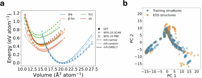
a Calculated DFT and 1fi/mfi M3GNet energies of different silicon crystals as a function of the normalized volume. All predicted SCAN energies are relative to the lowest DFT energy of the diamond structure, while the zero of predicted PBE energies is shifted to the lowest energy prediction. b Visualization of the first two principal components of the encoded features using the M3GNet formation energy model for isotropically deformed crystals (“EOS structures”) and training structures.

Full size image

Pressure-induced phase transition of amorphous silicon

Amorphous silicon is known to undergo pressure-induced phase transitions. Here, isothermal compression MD simulations were performed on amorphous silicon cells containing 1728 atoms (see Methods section). Figure 7a shows the volume change of amorphous silicon under a uniform pressurization rate of 0.05 GPa ps⁻¹ with the various M3GNet GLPs. It can be observed that MD simulations using both 10%-mfi-random and 10%-mfi-DIRECT successfully reproduce the phase transitions observed in 80%-1fi-SCAN and previous work using MD simulations with a Gaussian Approximation Potential (GAP) on 100,000 amorphous silicon atoms⁵⁵. For instance, a volume collapse to very-high-density amorphous (VHDA) states is observed at ~ 15 GPa, and recrystalliization is observed with further compression. MD simulations with the 10%-mfi-narrow M3GNet GLP, on the other hand, predict the structural collapse to occur at a much lower pressure (~ 7 GPa), and no recrystallization was observed with further compression. From Fig. 7b, we can observe a sharp increase in potential energy at the phase transition pressure. This is followed by a small drop in potential energy with recrystallization in the 10%-mfi-random and 10%-mfi-DIRECT simulations, while no such drop was observed in the 10%-mfi-narrow simulations. Additionally, we note that the 80%-1fi-PBE model predicts the phase transition around 8 GPa, which is noticeably lower than those predicted by other SCAN GLPs.

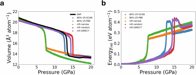
The evolution of (a) normalized volume and (b) potential energy of amorphous silicon with 1728 atoms is simulated by increasing the pressurization rate = 0.05 GPa ps⁻¹ from 0 GPa to 20 GPa. The energies are relative to the lowest energy of snapshots during pressurization. The simulated volume using Gaussian approximation potential (GAP) is reproduced from ref. ⁵⁵.

Full size image

Figure 8 shows that the local environments of structures extracted from simulations under 20 GPa at 500 K using all three GLPs. From Fig. 8b, it can be clearly observed that the structures extracted from the 10%-mfi-random and 10%-mfi-DIRECT simulations exhibit a clearly crystalline nature with lower coordination numbers (7 ≤ N_c≤ 8), while the structure extracted from the 10%-mfi-narrow simulation appears to remain amorphous with a greater percentage of highly coordinated Si atoms (N_c > 8). This poor performance of the 10%-mfi-narrow GLP can be attributed to the underestimation of short-range repulsive forces as can be seen in the relatively flat curvature of EOS curves (Fig. 6b) and the underestimation of the energy of high energy structures (Fig. 5a). MD simulations with the 80%-1fi-PBE also do not result in the formation of crystalline structures, highlighting the qualitative differences between the GLPs trained on PBE and SCAN functionals.

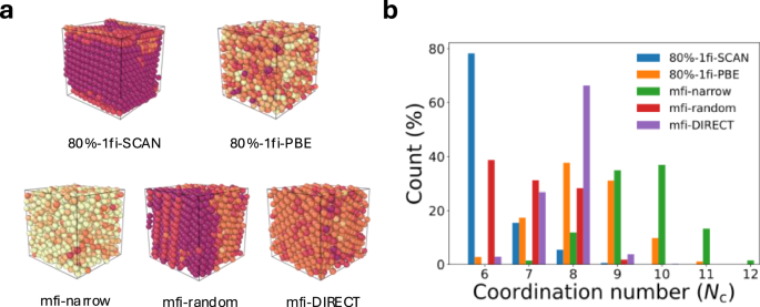
a The snapshot of isothermal compressed silicon structures. The heat map indicates the coordination number with a spatial cutoff = 2.85 Å. b The statistic of coordination number is obtained from 100 ps NPT simulations. The structures with color coding were visualized using Ovito⁷⁸.

Full size image

Interestingly, the 10%-mfi-random structure contains about 40% of atoms in a sixfold-coordinated β-Sn-like phase and 30% as sevenfold coordinated and eightfold-coordinated simple hexagonal (sh)-like phase. The 10%-mfi-DIRECT structure contains around 65% of atoms as eightfold-coordinated sh crystallites, 25% in sevenfold coordination, and the remaining atoms in a sixfold-coordinated β-Sn-like phase. The 80%-1fi-SCAN structures contain more than 75% of the atoms in the β-Sn-like crystal. The larger variations in the coordination distribution between the different SCAN GLPs can be attributed to the very small energy difference between the β-Sn and sh crystals, as seen in the EOS results, as well as sensitivity in the coordination analysis. Nevertheless, the main observation is that the mfi M3GNet models successfully reproduce the pressure-induced phase transition of disordered silicon observed in the 80%-fi-SCAN and DFT-SCAN simulations, unlike the 80%-1fi-PBE and 10%-mfi-narrow models.

Water

In this section, we develop mfi and 1fi M3GNet GLPs for water. Given the relatively similar performances of DIRECT and random sampling for the mfi M3GNet GLPs for silicon, only random sampling was used to select hifi training data for water.

Energy and force errors

Figure 9 shows the convergence of the energy and force MAEs of mfi M3GNet models for water with respect to the percentage of hifi (SCAN) data. The parity plots of energies and forces for all GLPs are provided in Figs. S4, S5. The 10%-mfi M3GNet has energy and force MAEs of 0.2 meV atom⁻¹ and 0.014 eV Å⁻¹, respectively, which is less than half those of the 10%-1fi model and outperforms even the 80%-1fi M3GNet GLP.

The test mean absolute errors (MAEs) of mfi M3GNet GLPs trained with different percentages of SCAN data for silicon. The dashed lines represent the MAEs of the 1fi M3GNet potential trained on 10%, 50% and 80% of SCAN data for reference.

Full size image

Structure of liquid water

NPT MD simulations were performed on a model containing 64 formula units of H₂O using the 10%-mfi and 1fi M3GNet IPs. Figure 10 compares the radial distribution functions (RDFs) of liquid water at 300K obtained using the mfi M3GNet GLPs and prior SCAN AIMD results. The 10%-mfi SCAN model is in agreement with 80%-1fi SCAN in terms of the position and magnitude of peaks. Notably, 10%-mfi SCAN predicted a lower first peak in the RDF of oxygen-oxygen, which better aligns with SCAN-AIMD results⁶⁴ compared to 80%-1fi SCAN. Similarly, the 10%-mfi SCAN generally matches the shape of the angular distribution function (ADF) of O-O-O with 80%-1fi SCAN as shown in Figure 11. Notably, the magnitude of peaks in the ADF predicted by 10%-mfi SCAN is even in better agreement with SCAN-AIMD⁶⁴. All these analyses show that the mfi M3GNet model enables the efficient construction of hifi MLPs with state-of-the-art accuracy using a fraction of data points, where the lofi dataset provides additional coverage in configuration space as shown in the first two PCs of reduced structural latent features from Fig. S6. The RDFs and ADFs at other temperatures can be also found in Figs. S7, S8, respectively.

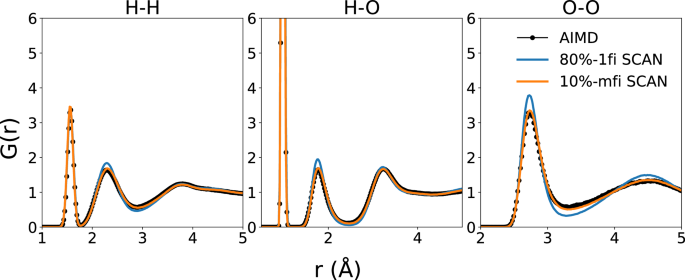
The RDFs were extracted from NPT simulations with the 80%-1fi and 10%-mfi M3GNet GLPs at 300K and 1 atm. The SCAN-AIMD results were obtained from ref. ⁶⁴.

Full size image

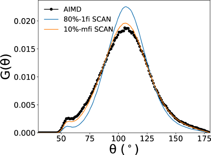
The O-O-O triplet angular distribution function of liquid water was computed with 80%-1fi SCAN and 10%-mfi SCAN at 300K and 1 atm. The AIMD results were obtained from ref. ⁶⁴.

Full size image

Structure of ice polymorphs

We also compared the performance of 10%-1fi-SCAN, 80%-1fi-SCAN and 10%-mfi-SCAN M3GNet with DFT-SCAN by conducting geometry relaxation on various small ice crystals (N_atoms < 100) reported in ref. ⁶⁵, which covers the majority of experimentally known phases. To measure the similarity between two crystal structures, we employed CrystalNN algorithm⁶⁶ to compute the structural fingerprint of periodic structures based on the Voronoi algorithm combined with the solid angle weights to determine the probability of various coordination environments. The smaller fingerprint distance indicates the higher similarity between the two crystal structures. Figure 12 shows the distribution of fingerprint distance among three different M3GNet models. The 10%-mfi SCAN generally achieves the lowest fingerprint distance between DFT-relaxed and M3GNet-relaxed structures among the three models. The main reason is that the lofi training set covers several crystal structures, which allows the mfi model to provide a more informative representation of local environments for other crystals resulting in better agreement with DFT-SCAN. In contrast, the other two models only contain the liquid water structures for training and therefore the extrapolation limits the accuracy of both models. The main reason is that the lofi training set covers various crystal structures. This enables the mfi model to offer a more informative representation of local environments for other crystals, resulting in better agreement with DFT-SCAN. In contrast, the training set for 1fi models only includes liquid water structures for training, which provides less accurate predictions for crystals.

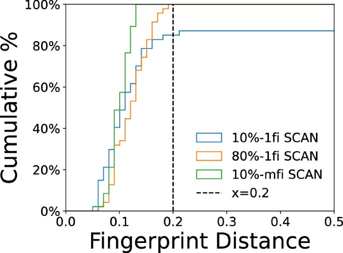
Cumulative histogram of calculated CrystalNN fingerprint distance between different M3GNet- and SCAN-relaxed ice structures. All these crystals are obtained from ref. ⁶⁵. The legend indicates the fraction of data points used for training. A smaller fingerprint distance means greater similarity between two relaxed structures and the vertical dashed line is used to visualize the fraction of structures that fall below 0.2 in terms of fingerprint distance.

Full size image

In the preceding sections, we have demonstrated that a multi-fidelity graph network architecture provides a data-efficient pathway to construct GLPs for higher levels of theory. From Figs. 3 and 9, we estimate that an mfi M3GNet GLP trained with a mfi dataset containing just 5–10% of SCAN data can achieve similar energy and force accuracies as a 1fi M3GNet GLP trained on a much larger 80% hifi SCAN dataset. This represents a savings of ~ 87.5 to −93.75% in the amount of hifi training data that needs to be computed. We note that lofi GGA-based data are often already available and the computational cost of a hifi SCAN calculation is several times higher than that of a lofi GGA calculation. Hence, the computational cost of constructing a hifi GLP is dominated by the cost of generating the hifi dataset.

Figure 13 compares the t-distributed stochastic neighbor embedding (T-SNE) analysis of the atomic features extracted from the silicon test set from a mfi and 1fi M3GNet trained on a 10% DIRECT SCAN data. Consistent with prior analyses, the mfi M3GNet model exhibits better separation between structures of high and low atomic energies in the latent space compared to the 1fi M3GNet model. We surmise that it is this improvement in latent representation with the inclusion of a large lofi PBE dataset that led to the improvement in the performance of the mfi M3GNet model.

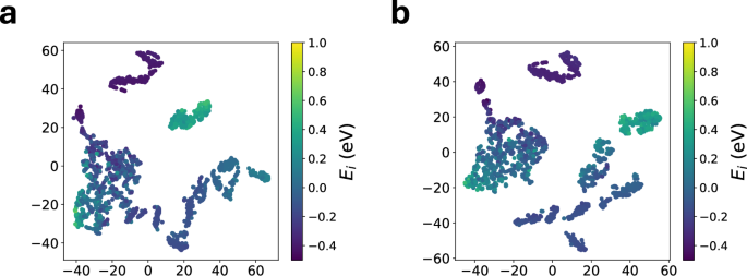
The atomic features for the test set of silicon were extracted from (a) 10%-1fi-DIRECT, and (b) 10%-mfi-DIRECT.

Full size image

As noted in the introduction, the mfi approach offers several advantages over transfer learning (TL) and Δ-learning. The mfi approach does not require an initial baseline model. It retains full model flexibility unlike the TL approach. And it does not require the same data to be generated in different fidelities like Δ-learning. Most importantly, a single mfi GLP can potentially be constructed for >2 fidelities, extracting the maximum value from scarce materials PES data. For comparison, we also trained two models using TL with the same 10% and 50% SCAN data (10%-TL and 50%-TL SCAN models, respectively). The same PBE training data was used for constructing the pretrained MLP, and the model weights in the embedding layer were fixed during the fine-tuning with SCAN data. The energy and force test MAEs of the 10%-TL SCAN model are 0.035 eV atom⁻¹ and 0.101 eV Å⁻¹, respectively, and those of the 50%-TL SCAN model are slightly lower at 0.031 eV atom⁻¹ and 0.097 eV Å⁻¹, respectively. In both cases, the corresponding mfi M3GNet models achieve slightly lower test MAEs in both energies and forces with the same amount of lofi and hifi data. This is likely due to the greater flexibility in the mfi model to learn the complex relationships between the lofi and hifi PESs, compared to the TL approach.

Though we have demonstrated the multi-fidelity concept using two relatively simple model systems (silicon and water), the impact of this work goes beyond custom MLPs for specific chemistries. For instance, a major area of active research is in the development of universal GLPs (also so-called “foundational” MLPs) with broad coverage of the periodic table of the elements. Generating a robust training dataset, even with standard GGA methods, for such universal GLPs is a major challenge. Using the multi-fidelity approach outlined in this work, we anticipate that training universal GLPs based on state-of-the-art meta-GGAs such as the SCAN functional can be made noticeably more data-efficient. This approach can also be extended to other GLP architectures through appropriate modification to include a global fidelity embedding feature and additional message-passing operations.

M3GNet architecture

The Materials 3-body Graph Network (M3GNet) model architecture has been extensively covered previously, and interested readers are referred to ref. ²⁰ for details. Only the major parameter settings used in this work will be discussed here. The distance cut-off that defines the edges e_ij and the angles between two edges e_ij and e_ik was chosen as 5 Å. The lengths of the node, edge, and global state feature vectors were set at 64, 64, and 16, respectively. The node feature vector is a learned embedding based on the atomic number of each atom, while the global state feature vector is a learned embedding based on the fidelity of the data. The bond angles were expanded using a spherical harmonic basis with m = 3 and l = 0. The number of message-passing blocks (comprising sequential three-body interactions, bond, atom and global state updates) is set to 3. The numbers of training parameters in the 1fi and mfi M3GNet models for silicon are 221,597 and 325,757, respectively, while those for water are 221,661 and 325,821, respectively. Each dense layer contains 64 output neurons that are fully connected from the input neurons. The update functions are modeled using gated multi-layer perceptrons (MLPs) that contain two layers with 64 neurons for each layer. Each updated atomic feature vector is fed into a 64-64-1 gated MLP to predict the corresponding atomic energy. The total energy is expressed as the sum of the atomic energies, while the forces and stresses are calculated by taking the partial derivatives of the total energy with respect to the atomic positions and lattice vectors.

Potential training

All model parameters were optimized using the Adam algorithm⁶⁷. The initial learning rate was set at 0.001. The cosine scheduler was used to gradually reduce the learning rate to 0.01 of the original value in 100 epochs. Early stopping of the model training was triggered when the validation loss did not reduce for 200 epochs. A batch size of 16 and 8 was used in the model training for silicon and water, respectively. However, a smaller batch size of 4 was used for mfi M3GNet training for water to avoid training crashes caused by excessive memory assumption. The loss function for the potential training was given by

where MSE represents the mean squared error loss function, E_total denotes the total energy of the system, N_atoms denotes the number of atoms, and F_i,α denotes the force component acting on atom i along the α = x, y, z axis.

E_f is obtained by subtracting the elemental reference energies E_elem from the total energy, via the following expression:

where n_elem is a row vector representing the number of each element in the structure. The elemental reference energies E_elem were fitted using linear regression of the target total energies, using the following expression:

where E_total is the matrix of total energies with dimensions N_struct × N_elem, N_struct is the total number of structures, N_elem is the total number of elements, and A is the composition matrix obtained by stacking n_elem for all structures.

To recover the total energy from the atomic energies, the following expression is used:

where the scaling factor σ is calculated by taking the inverse of the root mean square of all atomic force components from the training set.

DFT static calculations

All DFT calculations were performed using VASP (version: 6.3.2) with spin polarization. The projector augmented wave method⁶⁸ was employed to describe core and valence electrons with pseudopotentials. The electronic convergence criterion was set at 10⁻⁵ eV. For the Murnaghan equation of state for silicon crystals, the energy cut-off and k-spacing were chosen to be 800 eV and 0.2 Å⁻¹.

Geometry relaxation

For the high-throughput geometry relaxation of ice crystals with DFT, the ionic and electronic convergence were set to 0.05 eV Å⁻¹ and 10⁻⁴ eV, respectively. The conjugate gradient algorithm⁶⁹ was employed to update the ionic positions. Moreover, the energy cutoff and k-spacing were chosen to be 0.35 Å⁻¹, respectively. The same force threshold was applied to the M3GNet geometry relaxation via ASE interface⁷⁰ using the LBFGS⁷¹ algorithm.

MD simulations

All MD simulations were performed with LAMMPS^72,73 (version: 2Jun2022). A Nose-Hoover thermostat was employed to control temperature and pressure for NPT simulations. The time step was chosen to be 1 fs and the damping constants for temperature and pressure were set to 0.1 ps and 1.0 ps, respectively.

Amorphous silicon structures were generated by the melt-and-quench approach. The initial structure was obtained by random displacement of 1728 silicon atoms in the cubic cell with a density of 2.56 g/cm³ and then relaxed under a force threshold of 10⁻³ eV Å⁻¹. The relaxed structure was equilibrated at 1500 K for 110 ps and then cooled down to 500 K. A fast quenching rate of 10¹³K s⁻¹ was used for quenching from 1500 K to 1250 K and from 1050K to 500K, while a slower quenching rate of 10¹¹K s⁻¹ was used for quenching from 1250 K and 1050 K. The simulated temperature and the corresponding potential energy of silicon during the melt-and-quench are provided in Fig. S3. After an additional 50 ps equilibration at 500K, the amorphous silicon was isotropically compressed at a rate of 0.05 GPa (ps)⁻¹ from 0 GPa to 20GPa. The snapshot of silicon structures at 20 GPa was further equilibrated for 20 ps at 500K. Finally, their structural properties were obtained from 100-ps NVE simulations. For the NPT simulations of liquid water, an initial cubic cell containing 64 H₂O molecules with ρ = 1.0 g cm^-3 was equilibrated for 50 ps under 1 atm. The density and structural properties were extracted from a production run of 0.5 ns.

DIRECT sampling

The DImensionally-Reduced Encoded Clusters with sTratified (DIRECT) sampling workflow has already been detailed in previous work⁷⁴. First, a pre-trained M3GNet Materials Project formation energy model was used to encode structures into a 128-element vector. Next, principal components analysis (PCA) was performed on the encoded structure features, and the first six PCs with eigenvalues greater than 1 (Kaiser’s rule) were selected as a reduced-dimensionality representation. Finally, the balanced iterative reducing and clustering using hierarchies (BIRCH) algorithm⁷⁵ was used to divide all encoded structures into n clusters and k structures are sampled from each cluster for static DFT calculations. In this work, the values of n, k, and the threshold used to construct the 1fi and mfi M3GNet GLPs of silicon are given in Table S1.

Training data selection

For silicon, 80% of the training structures were selected from a total of 608 structures, with 70% randomly sampled and 10% DIRECT sampled to ensure the training set covered mostly diverse structures while keeping sufficient structural diversity for meaningful validation and testing. The hifi SCAN data points for training the 10%-mfi-narrow M3GNet model were selected based on PCA, where their first and second PC values were lower than -12.5 and -2.5, respectively. As for water, all training structures were randomly sampled for constructing 1fi and mfi M3GNet GLPs.

T-SNE visualization

The t-Distributed Stochastic Neighbor Embedding (t-SNE) analysis was performed using the OpenTSNE library^76,77. The cosine distance was used as the distance metric. All other settings were kept at the default values.