Decoupling of surface water storage from precipitation in global drylands due to anthropogenic activity
Main
Encompassing about 45% of Earth’s terrestrial land surface1 and supporting over three billion people, drylands are vital components of Earth’s system; yet they face notable challenges due to limited water resources2,3. Characterized by a high ratio of evapotranspiration (water loss) to precipitation, these regions possess only 7.7% of the world’s renewable surface water4. This scarcity markedly impacts both human well-being and the health of vulnerable dryland ecosystems5,6. Furthermore, increasing atmospheric and human water demands exacerbate regional water scarcity7.
Despite the vulnerability of drylands to water scarcity, our understanding of long-term surface water storage trends remains limited. Existing research often focuses on water area changes8 or assesses storage changes in a relatively small number of specific lakes and reservoirs9,10,11. Whereas helpful, these approaches are limited in their usefulness for comprehensively understanding past changes and developing effective adaptation strategies for the future3,12. Identifying the key drivers behind changes in surface water storage is crucial for understanding and managing water resources in drylands. These changes are influenced both by precipitation patterns, driven by large-scale atmospheric processes13,14, and by land-surface dynamics, such as irrigated agriculture15. On a smaller scale, factors such as evapotranspiration, run-off and water-management practices (for example, reservoir operation and water diversions) all play crucial roles in shaping dryland water availability16,17,18.
Whereas short-term variations in surface water storage primarily reflect precipitation fluctuations19, long-term trends are influenced by local hydrological processes and human water management. Studies based on models have reported a decoupling of precipitation from surface water storage in some regions20,21,22. However, accurately attributing long-term changes, particularly at larger scales, remains challenging due to uncertainties in how models represent human activities such as irrigation, which accounts for about 90% of human water consumption globally, alongside other complex processes including reservoir operations.
Here we provide an observation-based assessment of surface water storage trends in global drylands from 1985 to 2020. We then attribute observed changes to alterations in (1) precipitation, which reflects the natural sources of atmospheric water supply; (2) watershed hydrology, which includes local processes such as evapotranspiration and run-off and (3) water management, which refers to human interventions such as reservoir operations. To achieve this, we develop a global dataset from multi-mission remote sensing data. This dataset contains monthly active storage changes, which we represent as the water volume above the lowest level observed during the examined period for 105,400 water bodies (total capacity of 5,450 km3) in global drylands. These include 95,383 natural lakes and 10,017 reservoirs (Supplementary Fig. 1). The attribution analysis then compares the water storage change at a river basin scale to precipitation change, change in storage-to-precipitation ratio (which reflects the combined effect of watershed hydrology and human water management), change in streamflow-to-precipitation ratio (which we use to identify the impact of watershed hydrology) and change in storage-to-streamflow ratio (which isolates the impact of human water management on water storage changes).
Surface water trends in global drylands
We find that surface water storage in global drylands has increased by 2.20 km3 yr−1 (p < 0.05) from 1985 to 2020 (Fig. 1a), primarily due to the construction of new reservoirs (1.81 km3 yr−1, p < 0.05; Fig. 1b)23,24. These new reservoirs were mainly constructed during the 1980s and 1990s (Fig. 1b). Lakes and reservoirs that were present before 1983, on the other hand, do not contribute significantly to the growth of active storage (lakes: 0.28 km3 yr−1, p > 0.05; pre-1983 reservoirs: 0.12 km3 yr−1, p > 0.05).
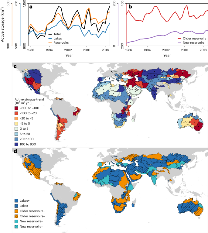
a, Annual changes in active storage for total (that is, lakes and reservoirs) surface water, lakes and reservoirs. b, Annual changes in active storage for older and new reservoirs. c, Long-term trend for total active storage for the 128 basins in global drylands. d, Attribution of the long-term trend to lakes, older reservoirs and new reservoirs. Lakes and reservoirs were differentiated according to the HydroLAKES dataset and the GOODD dataset. The new reservoirs were defined as reservoirs constructed in 1983 or later whereas older reservoirs were those constructed before 1983, which is chosen as two years prior to 1985 to account for the impoundment period. Basins are represented by the HydroBASIN Level-3 basins. In c, the stippling marks basins for which the long-term trend is statistically significant (with non-parametric Mann–Kendall test at a significance level of 0.05 and a sample size of 36). In d, the ‘+’ represents a positive effect and the ‘−’ represents a negative effect. Basemaps in b and c from World Bank Official Boundaries under a Creative Commons licence CC BY 4.0.
Total active storage also displays large inter-annual variability, which is probably linked to large-scale climate oscillations (Supplementary Fig. 2). For instance, the peak storage from 1997 to 1999 coincided with the powerful El Niño that increased precipitation in arid regions25. Lakes and reservoirs have similar contributions towards the total inter-annual variability in global drylands. This contrasts with the seasonal variability, which is dominated by reservoirs10. Compared to lakes and older reservoirs (that is, pre-1983), new reservoirs show a notably smaller inter-annual variability. This is probably due to the limited impact of climate variability on reservoirs during their initial filling period.
Whereas active storage has increased in African and Central Asian drylands, it has decreased in the Southwestern United States, South America, the Middle East, northeastern China and Australia (Fig. 1c). For example, the Colorado River Basin in the United States has suffered from a megadrought (active storage trend of −0.75 km3 yr−1, p < 0.05), which started in 2000 and was caused by both climatic factors and human water management26,27. Similarly, Australia, especially the Murray–Darling River Basin, and the Middle East region have also shown decreasing active storage that has affected local agriculture and human water needs28,29. In contrast, most dryland regions in Africa, especially in the Saharan region, have experienced an increase in active storage, partially due to decadal monsoonal rainfall changes and human activity30,31,32. On a global scale, the basin-wise trends in active storage are highly consistent with the trends of terrestrial water storage33, suggesting consistent changes in surface water and total water storage for many regions34.
In most basins (116 out of 128, 91%), long-term trends in active storage of surface water are primarily driven by changes occurring in lakes and older reservoirs (Fig. 1d). This contrasts with the globally aggregated time series, where the trend largely results from the construction of new reservoirs (Fig. 1a,b). This contrast is mainly caused by the clustering of new and large reservoirs in several regions (such as Ethiopia, India and northern China), which collectively have constructed 321 new reservoirs (total capacity of 152 km3) since 1983 (Supplementary Fig. 3). These large new reservoirs contribute to the long-term growth of active storage in the global drylands (Fig. 1b). In regions without substantial new reservoir construction, lakes and older reservoirs dominate storage changes. For example, in the drylands of the southwestern United States, the storage changes in older reservoirs (for example, Lake Mead and Lake Powell) dominate the surface water trend in most basins. In regions such as Saharan Africa and Western Australia, the trend in surface water storage is mostly attributable to lakes due to the lack of large reservoirs in these regions.
Decoupling of precipitation and surface water storage
The long-term changes in surface water storage are generally consistent with changes in precipitation (Fig. 2a). Among the 128 basins in global drylands, 87 show consistent trends (in terms of directional change) between active storage and precipitation. However, the remaining 41 basins exhibit opposite directional change, suggesting a decoupling of surface water storage from precipitation.
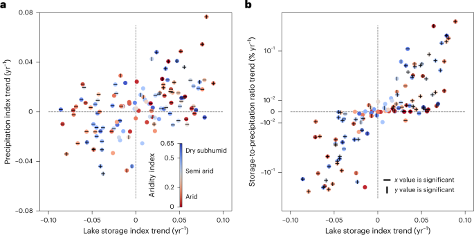
a, Relationship between the trend of SLSI and the trend of SPI. b, Relationship between SLSI trend and SPR trend, which represents the changes in land-surface process. SLSI and SPI were calculated by normalizing the monthly time series of active storage and precipitation, respectively. SPR was calculated for each basin by dividing total active storage by volumetric precipitation (that is, precipitation rate multiplied by area). The trends for SPR were quantified using multivariate robust regression by excluding the impacts of precipitation on SPR (Methods). Lakes and reservoirs were grouped based on the Aridity Index (AI) into Arid (0 ≤ AI < 0.2), Semi-arid (0.2 ≤ AI < 0.5) and Dry subhumid (0.5 ≤ AI < 0.65). Trend significance was assessed using the non-parametric Mann–Kendall test at a significance level of 0.05 and a sample size of 36 (years).
Such a decoupling is mainly caused by the changes in land-surface processes (including watershed hydrology and water management), as represented by the changes in water-storage-to-precipitation ratio, for which we have excluded the signal of precipitation (Methods and Fig. 2b). All these 41 basins exhibit consistent directional changes between storage and the ratio of storage to precipitation. Although changes in precipitation directly lead to changes in the volume of water that flows to lakes and reservoirs, water loss during surface routing and water-resources management in the river channels also impact long-term changes in surface water storage. Such a decoupling promotes changes to local management practices and highlights the importance of water conservation at a basin scale to counteract the impact of climate change.
For the 87 basins that show consistent directional changes between storage and precipitation, most of them (89%) also show consistent directional changes between storage and the ratio of storage to precipitation. This indicates that precipitation and land-surface processes jointly exert dominance over the long-term changes in surface water storage.
Whereas consistent with local-scale studies for a few basins17,35,36,37, our results contradict those related to global reservoirs, whose variability is mainly driven by precipitation change38, and thus highlight the distinctive nature of water balance in global drylands39. Such a contrast is probably caused by the larger influence of human activity on lakes and reservoirs in global drylands11,40. It is worth noting that we did not find a clear relationship between basin aridity and trends in the precipitation index, storage index or storage-to-precipitation ratio, implying that regional heterogeneity trumps the ‘dry regions get drier, wet regions get wetter’ paradigm in global drylands.
Attribution of changes in active storage
The changes in surface water storage are attributed to three driving factors including (1) atmospheric water supply (that is, precipitation), represented by the standardized precipitation index, (2) watershed hydrology, represented by the streamflow-to-precipitation ratio and (3) water management, represented by the storage-to streamflow ratio (Fig. 3 and Supplementary Table 1). For each factor in this chain of processes (that is, precipitation to streamflow and then to surface water storage), we exclude the signal from the previous processes (Methods) such that the trend in the ratios isolate the change in a single factor in each case.
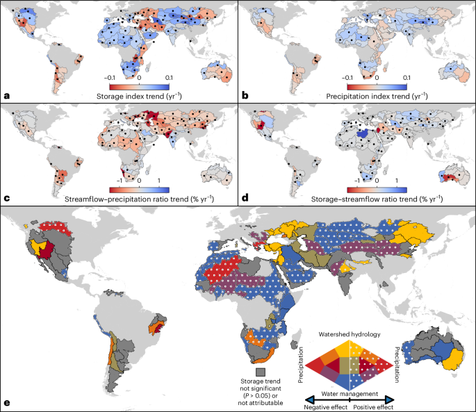
a, Trend in annual SLSI from 1985 to 2020. b, Trend in annual SPI from 1985 to 2020, representing the changes in precipitation. c, Trend in the ratio of streamflow to precipitation from 1985 to 2020, representing the changes in watershed hydrology. d, Trend in the ratio of active storage to streamflow from 1985 to 2020, representing the changes in water management. e, The major causes of surface water storage trend. Here surface water storage trend excludes the impact of new reservoirs. The dark grey colour in e indicates that the basin has an insignificant trend (with non-parametric Mann–Kendall test at a significance level of 0.05) in standardized lake storage index or the trend of standardized lake storage index is not attributable to the three factors (that is, insignificant trends for all factors). White stippling in e indicates that the factors have a positive effect, otherwise they have a negative effect. Detailed attribution information can be found in Supplementary Table 1. Basemaps from World Bank Official Boundaries under a Creative Commons licence CC BY 4.0.
Basins with a significant decreasing trend in surface water storage are mainly affected by watershed hydrology, which decreases streamflow under warming conditions (Fig. 3c,e). In some cases, changes in watershed hydrology are the only major factor (for example, the Murray–Darling River Basin in Australia or basins surrounding the Black Sea) (basin map in Supplementary Fig. 4), whereas in other watersheds, changes in watershed hydrology are observed together with decreasing precipitation (for example, Sao Francisco River Basin in South America) or water management (for example, basins surrounding the Caspian Sea; Supplementary Fig. 5). A unique example is the Colorado River Basin in the United States, where all three factors lead to a reduction in reservoir storage. Conversely, for the Tigris–Euphrates River Basin, decreasing storage is primarily attributable to human water management.
Human water management is probably the primary driver for the 52 basins with increasing active storage (Fig. 3d,e). These basins are clustered in Africa and Central Asia. Taking the Nile River Basin as an example, despite decreasing precipitation and increasing evapotranspiration, surface water storage has increased (0.068 km3 yr−1). This is probably due to improved management of the High Aswan Dam (forming Lake Nasser, the largest reservoir in Africa), especially after the severe drought in 1981–198841. In the arid Tarim River Basin in northwestern China, human water management, along with increasing precipitation (known as the ‘warming–wetting’ trend)42, has offset the impact of increased evapotranspiration and has led to an increase in surface water storage.
We find that human water management can lead to either an increase or a decrease in surface water storage. On one hand, intensive water diversion can exacerbate the warming-induced flow reduction and lead to more water stress. This represents a regional challenge for achieving the United Nation Sustainable Development Goals (for example, goals 6 and 14)43,44,45. Such an effect can be seen, for example, in the Tigris–Euphrates River Basin. On the other hand, more efficient water-resources management can offset the warming effect (although it may not be sufficient to counteract the impact of future warming)46,47. This can be observed, for example, in Spain. To this end, identifying human-induced and climate-induced water scarcity can assist targeted water-resources management, especially in the global drylands, where depletion of non-renewable groundwater has increased the reliance on surface water6.
We note that the result of our qualitative attribution analysis depends on the accuracy of input data, and particularly their trends. For lake storage, our validation (in terms of both variability and trends) has shown that remotely sensed data are sufficiently accurate to represent surface water dynamics. For precipitation, using an ensemble dataset rather than a single source enhances the reliability of trend analysis. The robustness of these two datasets supports our conclusion—the decoupling of lake storage from precipitation. Streamflow, derived from hydrological models, introduces greater uncertainty. Because it is an intermediate variable in the precipitation–streamflow–storage chain, however, this does not affect our main conclusion. Future studies could explore a quantitative attribution by modelling precipitation, streamflow and lake storage in an integrated manner to provide a more comprehensive understanding of the drivers behind changes in lake storage.
Overall, we find that anthropogenic activity, whether directly via flow regulation or indirectly via greenhouse gas emissions that increase temperature and evapotranspiration, has decoupled surface water storage from precipitation in global drylands. This decoupling highlights the emerging roles of global warming and human flow regulation in long-term changes in hydrological processes.
Water-resources management solely based on precipitation is thus likely to over- or under-estimate water availability. Instead, water-resources planning needs to integrate climate, watershed and society information in water-availability assessment. Regions with decreasing storage, and especially those regions exhibiting compound negative effects (for example, Southwestern United States, South America and Central Asia), need particular attention and will necessitate spatially nuanced water-management strategies to safeguard sustainable water access in these dry regions.
Methods
Lakes and reservoirs in global dryland
Global drylands are defined based on the Aridity Index (AI)48, which represents the ratio of precipitation and potential evapotranspiration (Supplementary Fig. 1). The basins from the HydroBASIN Level-3 basins that have an AI value smaller than 0.65 were used in this study and classified into three aridity categories: arid (0 ≤ AI < 0.2), semi-arid (0.2 ≤ AI < 0.5) and dry subhumid (0.5 ≤ AI < 0.65).
All lakes and reservoirs from the HydroLAKES dataset49 that intersect with the selected basins are included in the study, yielding 105,400 lakes and reservoirs. HydroLAKES differentiates lakes and reservoirs according to the GRanD dataset23. However, GRanD contains only 6,715 large artificial reservoirs, and thus, many small- to medium-size reservoirs were labelled incorrectly as lakes in HydroLAKES. Here we further use the GlObal geOreferenced Database of Dams (GOODD)50 dataset to label 7,188 additional artificial reservoirs in global drylands. We define ‘older reservoirs’ as those constructed before 1983, which is two years prior to the period covered in this study, that is, 1985, to consider the impoundment period. The ‘new reservoirs’ are defined as those with a construction in 1983 or later.
Remotely sensed lake hypsometry
The hypsometric curves for each lake were derived using multiple sources of satellite-based products (Supplementary Table 2). The surface water occurrence (SWO) image from the global surface water (GSW)8 dataset was used as the reference map. The SWO image was constructed by stacking historical (March 1984 to December 2020) monthly water classification maps and shows the probability of water coverage (0% to 100%) at each 30-m-by-30-m pixel at the global scale. Compared to a lake bathymetry image, a lake SWO image contains the same spatial pattern but without altitudinal information (Supplementary Fig. 6a). Here we developed a novel and globally applicable approach to convert the probability values from the SWO image to altitudinal values and then derived the hypsometric curves.
The altitude information was extracted and extrapolated based on the elevation information from four global Digital Elevation Model (DEM) maps. These include the NASA Digital Elevation Model (NASADEM), the Advanced Land Observing Satellite (ALOS) World 3D-30m (AW3D30), the Terra Advanced Spaceborne Thermal Emission and Reflection Radiometer (ASTER) Global Digital Elevation Model (ASTGTM), and the Copernicus Digital Elevation Model (COPDEM). These DEM maps were collected using different sensors at various periods ranging from 2000 to 2015 (Supplementary Table 2). Due to the differences of their data collection times, these four DEM maps may have captured different shorelines of the global water bodies due to the dynamics of water levels. This leads to different lake bathymetry exposures at the water body edges. For example, the Nath Sagar Lake, India, has the largest exposure of its bathymetry (that is, lowest water level) from AW3D30 (Supplementary Fig. 6b). However, such bathymetric exposures are insufficient to cover the full range of water dynamics of the SWO image, which is based on monthly area changes from March 1984 to December 2020.
To obtain hypsometric curves for the full dynamic range, we followed these steps:
-
1.
Establish occurrence–elevation relationships. We derived these relationships from the SWO image and each of the four DEM maps, represented by the four coloured lines (in Supplementary Fig. 6c). The horizontal lines indicate the lowest elevation exposed by each DEM.
-
2.
Select the optimal DEM. We identified the DEM with the greatest exposure of lake bathymetry. For Nath Sagar Lake, the AW3D30 DEM was selected.
-
3.
Extrapolate the occurrence–elevation relationship. We extended this relationship to encompass the full range of water occurrence in the SWO image (dashed line in Supplementary Fig. 6c). We retained the exposed bathymetry from AW3D30 and used only the ten highest occurrence values from the occurrence–elevation relationship for linear extrapolation.
-
4.
Reconstruct hypsometric curves. We established the area–elevation–storage relationship (Supplementary Fig. 6d) through the following sub-steps:
-
a.
The area corresponding to each occurrence value was calculated from the SWO image to create the occurrence–area relationship (Supplementary Fig. 6d2).
-
b.
This relationship was then combined with the occurrence–elevation relationship to generate the area–elevation relationship (Supplementary Fig. 6d3).
-
c.
Finally, using the area–elevation relationship as the integrand, we calculated the area–storage relationship through integration (Supplementary Fig. 6d4).
-
a.
Note that the storage value here is referenced to the largest occurrence value (that is, lowest water level during the 37 years from March 1984 to December 2020). Thus, it only shows the storage difference between an actual storage value and the minimum storage value from 1984 to 2020. For example, the largest occurrence value for Nath Sagar Lake is 100%, meaning the pixels with this occurrence value are constantly covered by water during the 37-year period. The storage at this occurrence value thus represents the minimum storage from March 1984 to December 2020. Here we used this minimum storage as the reference (that is, zero) and reported other storage values as the difference between their actual storage and this reference. It is also worth noting that different datums among DEMs (as shown in Supplementary Fig. 6c) do not affect the storage calculation as (1) we chose the optimal DEM rather than merging all DEMs and (2) the calculation of storage relies on the integral of elevation–area relationship (Supplementary Fig. 6d3) and shifts in this relationship—whether upward (lower datum) or downward (higher datum)—do not alter the calculation of integral storage.
The primary uncertainty in using this DEM-based method to derive hypsometric curves stems from the extrapolation of the occurrence–elevation relationship. To illustrate the extent of this extrapolation, we calculated the percentage of the occurrence range exposed by the optimal DEM relative to the entire occurrence range (Supplementary Fig. 7). Overall, the median percentage is 82.3%, indicating that the optimal DEM effectively represents the full dynamic range of lakes and reservoirs. However, lakes in North America, Eastern Europe and Southern Africa exhibit relatively low percentage values, suggesting their hypsometric relationships rely more on extrapolation.
Area, elevation and storage dynamics
The monthly surface area time series were generated based on our previously developed algorithms51,52 and the GSW) dataset8.
The GSW dataset8 offers monthly water coverage at a 30-m resolution globally from 1984 to 2020. However, these monthly water maps are often contaminated by clouds, cloud shadows, terrain shadows and sensor failures, resulting in data gaps (indicated as ‘no data’). Consequently, directly extracting data from GSW to generate area time series may lead to notable underestimations for many months. To mitigate this issue, we developed an image enhancement algorithm capable of automatically repairing contaminated water coverage through shoreline detection52.
Using Nath Sagar Lake (India) in September 2015 as an example, the raw water area shows the water classification result from GSW (Supplementary Fig. 8a). A large area of the reservoir was covered by cloud and cloud shadow and thus was reported as ‘No_data’ pixels in GSW. To correct such contamination issues, we first identified the visible coastline—pixels that are between ‘Water’ and ‘Land’—of the contaminated image (Supplementary Fig. 8b) and then used the SWO (Supplementary Fig. 8c) as the water-level reference map to extend the visible coastline to the cloud-cover area (Supplementary Fig. 8d). By applying this algorithm to each of the contaminated images from GSW from 1985 to 2020 for this reservoir, the ‘Enhanced’ area time series is obtained (Supplementary Fig. 8e). Compared to the ‘Raw’ time series, numerous underestimated area values (due to multi-source contamination) have been corrected.
The water area extraction algorithm was validated using synthetically contaminated images. These images were created by overlaying contaminated pixels from a randomly selected contaminated image onto a ‘true state’ image, which was free of contamination. We then applied our image enhancement algorithm to these synthetically contaminated images to delineate the full water extent. Since the actual water area is known from the ‘true state’ image, we could validate the delineated water area. This process demonstrated an average absolute relative error of 3.7%, indicating the high accuracy of our algorithm.
Using the derived area–elevation (Supplementary Fig. 6d3) and area–storage (Supplementary Fig. 6d4) relationships, the monthly elevation time series and storage time series can then be generated for each lake (Supplementary Fig. 8f).
Elevation and storage validation
We use in situ observed elevation data from multiple sources to validate the performance of our algorithm (Supplementary Fig. 9). We do not rely on the in situ reported storage data due to two critical considerations. First, in situ reported storage data are not from direct measurement. Instead, storage data are typically derived using measured elevation and an estimated elevation–storage relationship, which contains large uncertainties during the bathymetric survey that may not cover the whole range of elevation values. Second, in situ reported storage data are derived based on a certain boundary of the water body. However, for reservoirs that were constructed on rivers, there is no clear cutline to distinguish reservoirs from rivers. Such an issue is further exacerbated by the uncertainty of the HydroLAKES shapefile, which may not cover the entire water body. Thus, we use in situ observed elevation data for the validation of our algorithm because elevation is directly measured at in situ sites, and its uncertainty is irrelevant with the bathymetric survey and defined lake boundary.
The median correlation coefficient is 0.79 for 181 lakes that have more than 20 years of in situ measured elevation data (Supplementary Fig. 9a,b), showing that our algorithm can satisfactorily reproduce the temporal variability of elevational changes. The median root mean square error value is 2.43 m (the median dynamic range of observed elevation change is 12.85 m). The monthly time series for 36 lakes with different sizes, geographical locations, climate regions are shown in Supplementary Fig. 10, Supplementary Fig. 11 and Supplementary Fig. 12 and demonstrate the satisfactory agreement between in situ observed elevation and simulated elevation values. We also validate our storage product with a satellite-based product from Busker et al.9 (Supplementary Fig. 13), which paired satellite altimeter data with Landsat-based area classification. For the 30 lakes, the median correlation coefficient is 0.93, and the relative bias is −11%, indicating good agreement between the two datasets.
Because we primarily relied on storage time series trends for attribution analysis, we further validated the trend of simulated elevation values across 181 lakes (Supplementary Fig. 14). The results show a correlation coefficient of 0.90 and a root mean square error of 0.89 m per decade. Notably, the correlation coefficient for trends exceeds the median correlation coefficient for elevation time series, indicating that our method more accurately captures long-term changes in lake dynamics.
The uncertainty in storage calculation is mainly affected by the accuracy of hypsometry. Using multi-mission DEM data, the uncertainty from each of them can be minimized. In addition, we expect it has a limited impact on the long-term trend of active storage, especially at a basin scale. The long-term trend of active storage can also be affected by sedimentation, which is estimated to be 0.7% of storage capacity based on 21 reservoirs in the Missouri River Basin in the United States53. However, this process mainly affects the inactive storage instead of the active storage of lakes and reservoirs and thus has limited effect on the trend analysis in our work. It is also worth noting that glacier melting may contribute to the increasing trend of storage54. Given that only 18 basins (out of 128) have both glaciers and an increasing trend of storage, this process may have a limited effect on the global attribution analysis.
Calculation of indices and ratios
For a consistent comparison of surface storage change among different regions, and for comparison with precipitation and run-off indices, we convert the active storage time series to the standardized lake storage index (SLSI). The conversion was implemented by converting the empirical cumulative distribution function to a Gaussian distribution using the Probit Function34. It is worth noting that we did not use a specific distribution function (for example, Gamma or logistic distributions) for the active storage values because the spatial heterogeneity precludes the uniformity of such a distribution function.
We use four precipitation datasets to account for the uncertainty of different products (Supplementary Table 3). The precipitation time series for each basin was calculated by averaging the grids that overlap the basin boundary. Then, similar to the calculation of SLSI, the precipitation time series was converted to the standardized precipitation index (SPI), and the storage-to-precipitation ratio (SPR) time series was calculated using active storage divided by the volumetric precipitation (that is, precipitation rate multiplied by the basin area). To account for the hydrological lag between surface water storage and precipitation, we calculate the time lag by optimizing the correlation coefficient between the monthly SLSI and SPI (Supplementary Fig. 15). Then a lagged SPI time series that maximizes the cross-correlation coefficient is used.
For streamflow, we use the Global Flood Awareness System (GloFAS) dataset, which couples the Hydrology Tiled ECMWF Scheme for Surface Exchanges over Land (HTESSEL) land-surface model and the LISFLOOD hydrological model. GloFAS provides daily river discharge at 1/10° spatial resolution from 1979 to the present. The streamflow time series was calculated by summing the flow values at all outlet grids in a basin. Then the volumetric lake evaporation (calculated after Zhao et al.55) was subtracted from the total streamflow. Similar to the calculation of SPR, the streamflow-to-precipitation ratio (FPR) time series was calculated by dividing the streamflow by the volumetric precipitation and the storage-to-streamflow ratio (SFR) time series was calculated by dividing active storage by streamflow. The three ratios (that is, SPR, FPR and SFR) were calculated on an annual basis instead of monthly to reduce the impact of extremely low (for example, zero) precipitation values in certain months and to reduce the impact of temporal autocorrelation and lags.
The GloFAS streamflow data were used to provide a globally consistent framework for analysing long-term hydrological changes, particularly in regions where observational streamflow data are sparse or absent. Uncertainties in the data, arising from the relatively coarse meteorological forcing and model parameterization, may affect the accuracy of streamflow simulations. However, as an intermediate variable in the precipitation–streamflow–storage chain, its uncertainty does not notably affect our main conclusion—the decoupling of storage and precipitation. We note that however, future research needs to focus on improving streamflow simulations (for example, employing ensemble global hydrological models that explicitly simulate lakes and reservoirs) that can enable quantitative, rather than qualitative as in this study, attribution of changes in surface water storage.
Trends in indices and ratios
We calculate the trends for both storage and precipitation by applying robust linear regression on the annual time series of corresponding indices (that is, SLSI and SPI). By using index time series instead of actual time series, the trend quantification can reduce the impact of inter-basin discrepancy and assist comparisons among basins (Fig. 2a).
For trends of ratios (that is, SPR, FPR and SFR), we calculate slope coefficients (that is, b1, b2, b3) for the variable Year by establishing multivariate robust linear regression (equations (1), (2) and (3). Such a regression method can remove the impact of precipitation on SPR and FPR, and the impact of flow on SFR.
where ({a}_{1}), ({a}_{2}), ({a}_{3}) are slope coefficients for precipitation and streamflow; ({b}_{1}), ({b}_{2}), ({b}_{3}) are slope coefficients for year; and c1, c2, c3 are intercept coefficients. Here we take the widely used flow-to-precipitation ratio as an example. Due to increasing marginal return of precipitation, the flow-to-precipitation function generally shows a convex, monotonically increasing curve56. As a result, FPR also increases with precipitation but typically in a linear form (the following paragraph provides more discussion). In such a case, a decreasing FPR is attributable to a decreasing precipitation and/or an increasing evapotranspiration. Here we use the partial slope coefficient for the variable Year excluding the linear effect of precipitation in the trend of FPR. Similarly, we exclude the impact of precipitation on the trend of SPR and the impact of flow on the trend of SFR.
In addition to the multivariate linear regressions in equations (1), (2) and (3), we also tested for non-linear partial relationships between SPR and precipitation, FPR and precipitation and SFR and streamflow. For this, we used Generalized Additive Models57 to refit the three equations using splines and inspected the effective degree of freedom of these three relationships. We used splines with an extra penalty so that the whole partial effect can be shrunk to zero in case it does not add any information to the model58. The results show that the majority of the river basins (that is, 88%, 76% and 79% for the three relationships) have an effective degree of freedom value close to 1 (Supplementary Fig. 16), indicating the validity of the linearity assumption. Examples for the Colorado, Missouri, Tigris–Euphrates, Orange–Senqu and Murray–Darling river basins are shown in Supplementary Figs. 17, 18 and 19. No nonlinearity was detected for any of these five river basins and three relationships.
Ethics and inclusion statement
All collaborators of this study that fulfil authorship criteria required by Nature Portfolio journals have been included as authors. Roles and responsibilities were agreed among collaborators ahead of the research.

Responses