Dephasing enabled fast charging of quantum batteries

Quantum thermodynamics lies at the intersection of fundamental and applied aspects of quantum information science and technology. This is evident from the problem statements in the field which are typically structured around microscopic versions of macroscopic machines like heat engines, refrigerators, batteries, etc. While the practical utility of such quantum thermal machines is still nascent, the fundamental aspects uncovered by studying them are expected to influence the design and optimization of current and future quantum devices¹. In this context, a central goal of the field has been to uncover phenomena that are unique or advantageous in quantum thermal machines such as heat engines, refrigerators, and batteries with no simple counterpart in the classical world^1,2,3. In the specific case of quantum batteries (QBs), which are quantum systems that store energy and are charged by direct parametric driving or via ancillary quantum charger systems, significant effort has been devoted to identifying situations where figures of merit such as the total energy and ergotropy that can be stored, charging and discharging time, and charging power are optimized^{2,4,5,6,7,8,9,10,11,12,13,14,15,16,17,18,19,20,21,22,23,24}.

While early studies of quantum batteries modeled the charging and discharging processes using closed unitary dynamics, there has been a concerted effort recently to extend this paradigm by including dissipative effects^{25,26,27,28,29,30,31,32,33,34,35,36,37,38,39,40,41,42,43,44}. One motivation to include dissipation stems from the recognition that all realistic quantum battery systems will be subject to interactions with their environment and it is imperative to assess and, if possible, mitigate the negative impact of the resulting dissipation on the battery’s performance^{26,27,28,30,34,41,44}. In contrast, viewing dissipation as a resource, recent works^{25,29,33,35,36,37,38,40,42,43,45} have highlighted the possibility of charging advantages for dissipative QBs under restricted settings such as specific models of dissipation^33,37, collective effects^29,36,37,42, control schemes^32,38, or particular choices of battery systems^35,40. Nonetheless a simple strategy to obtain fast and stable charging applicable to a wide variety of systems is missing. Exploring such strategies, especially regarding the limits on the charging time, can also draw from and provide connections to fundamental aspects of quantum dynamics like the quantum speed limit^46,47,48.

Here, we address this challenge by proposing a universal method to obtain fast charging of a quantum battery connected to a driven quantum charger system (shown schematically in Fig. 1) by controlled pure dephasing of the charger. We note that pure dephasing is one of the fundamental decoherence channels for open quantum systems⁴⁹ and involves the damping of off-diagonal elements of the density matrix. Pure dephasing is principally generated by the coupling of an operator that commutes with the system Hamiltonian, often taken to be the Hamiltonian itself, with a noisy environment^50,51,52. At small values of dephasing, as long as the charger-battery system is initialized in any state apart from the eigenstates of the total Hamiltonian, we expect coherent underdamped oscillation of the battery’s energy. In contrast, viewing the pure dephasing process as a continuous measurement of the charger’s energy by the environment, strong dephasing naturally leads to a quantum Zeno freezing of the charger’s energy and consequent suppression of the rate of charging of the battery. Thus for any charger and battery system, at an in-between moderate value of dephasing that provides a balance between the two effects, we expect to see an optimum fast charging of the battery. This is akin to the working of a shock absorber in a car where adding a dissipative element with the appropriate amount of damping ensures a smooth transfer of mechanical impulse. We confirm and illustrate our general strategy of dephasing-enabled fast charging by choosing the battery and charger systems as two-level systems (TLS) here and demonstrate its wider applicability in the Methods section and the Supplementary Material (SM) with quantum harmonic oscillators (HO) and hybrid TLS-HO setups. Moreover, we also find that the dephased charger lends a certain degree of robustness to the charging process when the charger or its driving is detuned with respect to the battery.

Schematic of the setup of a quantum battery B coupled to a quantum charger system C with a coupling constant g. The charger is driven at a strength F and additionally subject to dephasing at the rate γ_C.

Full size image

Setup

We consider a charger-mediated quantum battery setup consisting of a charger system C, and a quantum battery B (see Fig. 1). The Hamiltonian of the total system has the general form: (hat{H}(t)={hat{H}}_{{rm{C}}}+{hat{H}}_{{rm{d}}}(t)+{hat{H}}_{{rm{B}}}+{hat{H}}_{{rm{CB}}}). Here ({hat{H}}_{{rm{C}}}) and ({hat{H}}_{{rm{B}}}) denote the bare Hamiltonians of the charger and battery system respectively, ({hat{H}}_{{rm{d}}}) provides the coherent driving of the charger system that is the energy source, and ({hat{H}}_{{rm{CB}}}) gives the coupling Hamiltonian between the charger and battery that enables the charging process. In addition to the unitary dynamics generated by (hat{H}), the charger system undergoes a pure dephasing process that will be described via a Gorini–Kossakowski–Sudarshan–Lindblad (GKLS) master equation with a hermitian jump operator ({hat{L}}_{{rm{C}}}) that satisfies ([{hat{L}}_{{rm{C}}},{hat{H}}_{{rm{C}}}]=0). Thus the time evolution of the density matrix (hat{rho }) describing the charger and battery system is given by

with γ_C giving the rate of dephasing and { ⋅ , ⋅ } denoting the anticommutator (we take ℏ = 1 throughout). Taking the jump operator as ({hat{L}}_{{rm{C}}}propto {hat{H}}_{{rm{C}}}), allows the interpretation of the pure dephasing process in Eq. (1) as resulting from a continuous weak measurement of the energy^53,54 of the charger system. In Supplementary Section I of the SM, we provide a detailed derivation of the master equation based on this interpretation.

Starting with the charger and battery system in their respective (free) ground states, the evolution generated by Eq. (1) leads to an increase in the energy and ergotropy of the battery system that are defined as ({E}_{{rm{B}}}={{rm{Tr}}}_{{rm{B}}}[{hat{rho }}_{{rm{B}}}{hat{H}}_{{rm{B}}}]) and ({{mathcal{E}}}_{{rm{B}}}={E}_{{rm{B}}}-mathop{min }nolimits_{{hat{U}}_{{rm{B}}}}{{rm{Tr}}}_{{rm{B}}}[{hat{U}}_{{rm{B}}}{hat{rho }}_{{rm{B}}}{hat{U}}_{{rm{B}}}^{dagger }{hat{H}}_{{rm{B}}}]), respectively. Here, ({hat{rho }}_{{rm{B}}}equiv {{rm{Tr}}}_{{rm{C}}}[hat{rho }]) is the reduced density matrix of the battery and the ergotropy is defined by minimization over all possible unitaries ({hat{U}}_{{rm{B}}}) in the battery’s Hilbert space. Apart from the values of energy and ergotropy that serve as the standard figures of merit to describe the charging performance, we are specifically interested in the charging time τ of the battery which we define as

with E_B(∞) denoting the steady state energy of the battery and n > 0 an integer that we can choose. Note that Eq. (2) can in general have multiple solutions. In our considerations henceforth, we will take τ as the last root of Eq. (2) such that ∣E_B(t) − E_B(∞)∣ < e⁻ⁿ∣E_B(0) − E_B(∞)∣ for all t ≥ τ. This ensures that we do not underestimate the charging time. Since achieving the steady state within the GKLS master equation description requires infinite time in principle, our definition of τ in Eq. (2) is one practical way to estimate the charging time as the time scale over which the transient dynamics of the system settles down and the system’s energy approaches the steady state value within some tolerance.

To exemplify our results regarding the charging advantages with a dephased charger, we choose the battery and charger as two-level systems with the Hamiltonian

with ({hat{sigma }}_{{rm{B,C}}}^{-}={({hat{sigma }}_{{rm{B,C}}}^{+})}^{dagger }) representing the Pauli lowering and raising operators, ω_B (ω_C) giving the frequency of the battery (charger), and F, ω_d denoting the strength and frequency of the charger drive. When ω_B = ω_C (resonance), the battery-charger coupling in Eq. (3) commutes with the bare Hamiltonian of the battery and charger ensuring that there is no energetic cost to switch on/off the interaction in the absence of the driving. In addition, the jump operator that gives the pure dephasing in Eq. (1) is taken as ({hat{L}}_{{rm{C}}}={hat{sigma }}_{{rm{C}}}^{+}{hat{sigma }}_{{rm{C}}}^{-}). The energy and ergotropy of the TLS battery can be written as²⁸

and depend directly on the moments of the TLS operators. Hence, we study the dynamics and properties of energy and ergotropy by solving a closed set of equations for the moments (given in the Methods section) that follows from the master equation (1). We begin by considering the resonant case with ω_B = ω_C = ω_d, where we are able to get exact analytical solutions for the energy and ergotropy (see Methods).

Dephasing enabled fast charging

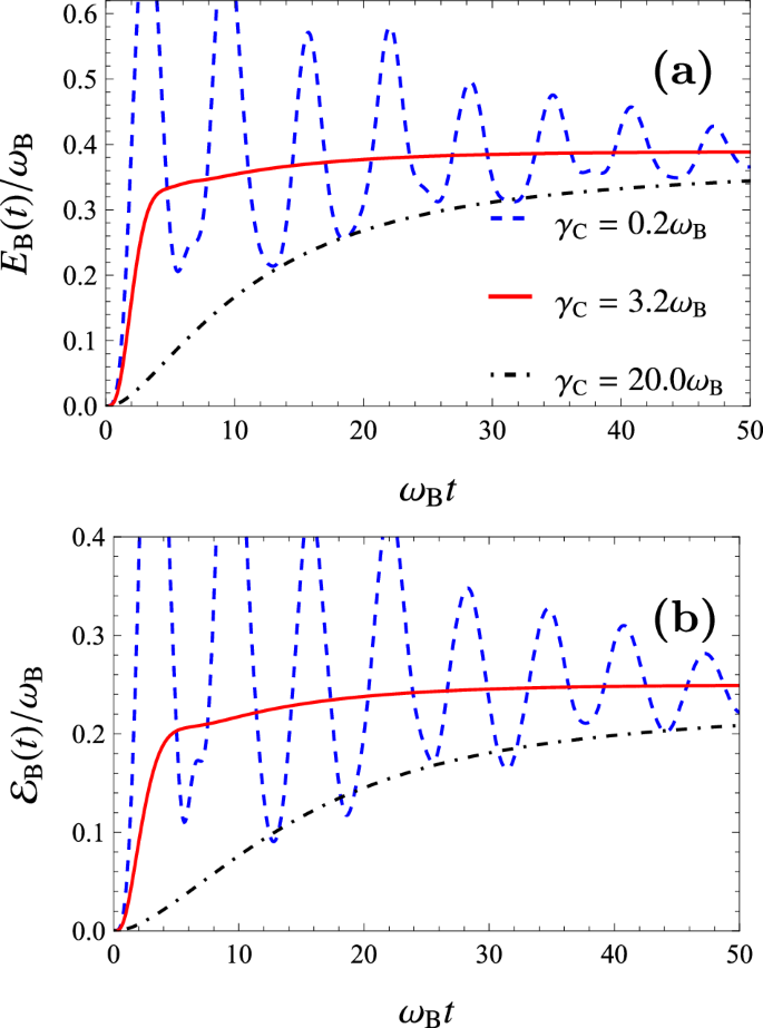
To illustrate our central result, we plot the time evolution of the average energy E_B (a) and ergotropy ({{mathcal{E}}}_{{rm{B}}}) (b) in Fig. 2 for different values of charger dephasing γ_C for a given value of the driving to coupling ratio F/g = 0.5 as an example. As evident from the plot, both ergotropy and average energy display underdamped oscillations for very small γ_C and slow overdamped behavior at very large γ_C. Crucially, at an intermediate optimal value of γ_C where the dynamics transitions from underdamped to overdamped, the ergotropy and average energy reach their steady values in the shortest time. A qualitative way to understand this behavior is to first note that in the limit where the dephasing is smaller than the interaction γ_C ≲ g, the persistent oscillatory exchange of energy between the charger and battery, for our choice of the initial state, dies down slowly leading to slow charging. On the other hand, large dephasing γ_C ≫ g, leads to the charger energy becoming constant due to the quantum Zeno effect. This naturally suppresses the battery charging leading to very slow transfer of energy to the battery. A moderate dephasing rate, as we anticipated, provides a trade-off between the two effects leading to fast charging of the battery. While here we have picked a particular value of F/g for demonstration, this main result holds for any value of F/g as well (see Supplementary Section II of the SM for details).

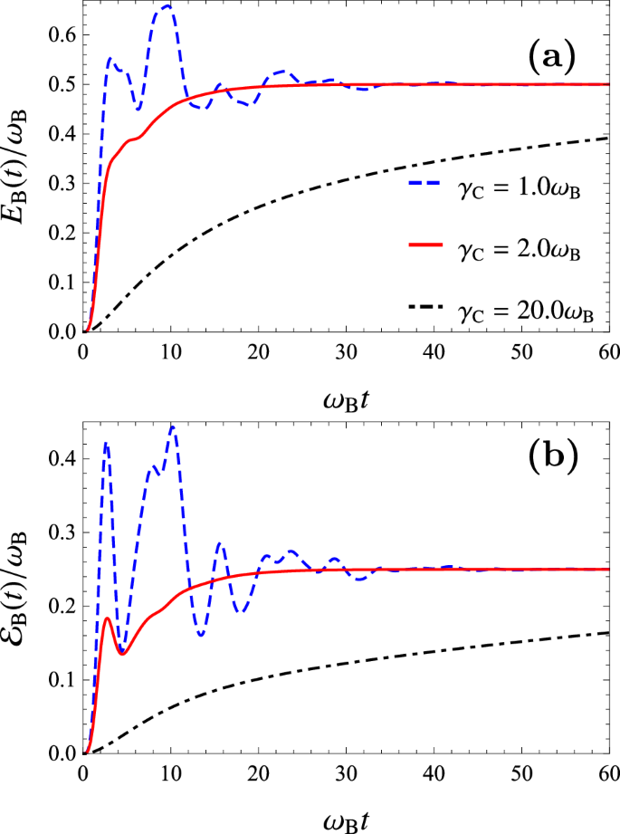
Time evolution of average energy E_B(t) (a) and ergotropy ({{mathcal{E}}}_{{rm{B}}}(t)) (b) of the battery for the two-TLS model for different values of the dephasing rate γ_C. Here, as an example, we show the resonant case, i.e. ω_C = ω_d = ω_B, for the optimal driving with F = 0.5ω_B, and g = 1.0ω_B (F/g = 0.5).

Full size image

Before turning to a detailed analysis of the charging time τ, we first note that for resonant driving the steady state value of the energy is ({E}_{{rm{B}}}(tto infty )/{omega }_{{rm{B}}}=frac{1}{2}) and the same for the ergotropy takes the form ({{mathcal{E}}}_{{rm{B}}}(tto infty )/{omega }_{{rm{B}}}=(F/g)/left(1+4frac{{F}^{2}}{{g}^{2}}right)). From this, it is easy to see that the steady state ergotropy is maximized for the optimal value of driving strength F/g = 0.5 chosen in Fig. 2, similar to previous work reported by Farina et al.²⁸. As evident from Fig. 2, during the transient dynamics the system’s energy can exceed or equal the steady-state values. We find that taking these transient crossings or maxima as charging times is impractical for two reasons. Firstly, the transient nature of the dynamics means that a small perturbation about the identified charging time can lead to much smaller energy values. Secondly, charging the battery to such transient time-instants would require fine tuning of the coupling time between the charger and battery. Moreover, assuming that we can control the coupling time very precisely, quickly removing the coupling between the charger and battery to stop the energy transfer affects the state of the battery, i.e., energy injection/removal by the turning couplings on/off cannot be avoided. Our definition of charging time clearly avoids these issues. As the first step to systematically study the behavior of the charging time and the optimal value of dephasing, we calculate τ by numerically finding roots of Eq. (2). While the typical choice of n = 1 in Eq. (2) describes the convergence of the energy to its steady value to one natural logarithm decade, we find that for scenarios with oscillatory terms of higher amplitude, a larger n gives a smoother variation of charging time as other parameters like the dephasing rate are varied. We plot charging time τ, calculated from Eq. (2) with n = 18, as a function of the dephasing rate γ_C in weak [Fig. 3a], strong [Fig. 3b], and intermediate [Fig. 3c] (which maximizes steady state ergotropy) driving strength regimes, respectively. In all three regimes, we can see that the charging time is minimized at a given optimal value of dephasing, denoted as ({gamma }_{{rm{C}}}^{star }) henceforth, underscoring our central result that moderate dephasing leads to fast charging. Additionally, we note that taking even larger values of n > 18 in the calculation of τ will only make the behavior of the charging time in Fig. 3 smoother but not affect any of the important qualitative features, especially the value of ({gamma }_{{rm{C}}}^{star }) (see in particular Fig. 3c where the scattering of the data points is still discernible).

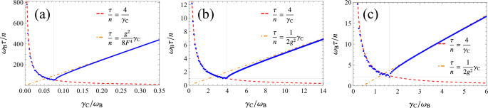
Charging time τ of the battery for the two-TLS model as a function of the charger dephasing rate γ_C for different regimes of the driving strength: a weak driving F = 0.1ω_B, g = ω_B (F/g = 0.1), b strong driving F = 10.0ω_B, g = ω_B (F/g = 10.0), and c optimal driving F = 0.5ω_B, g = ω_B (F/g = 0.5). Here, we show the resonant case, i.e., ω_C = ω_d = ω_B. Gray vertical lines indicate the value, ({gamma }_{{rm{C}}}^{star }), of the optimal dephasing to get the fastest charging time.

Full size image

Exploiting the exact expression for the battery’s average energy, we next obtain analytic expressions for the charging time at large (γ_C ≫ g) and small dephasing (γ_C ≪ g) regimes. This will allow us to also provide explicit analytical estimates for the optimal dephasing rate ({gamma }_{{rm{C}}}^{star }). Leaving the details of the derivation to the Methods section, we note that in the small dephasing limit (γ_C ≪ g) the charging time scales as,

irrespective of the values of F and g. This is neatly illustrated in Fig. 3a–c, where the behavior of the calculated charging time compares well with the red dashed curve representing the scaling given by Eq. (6) at small γ_C. On the other hand, in the large dephasing limit (γ_C ≫ g), we find

This large dephasing scaling is clearly illustrated by the orange dash-dotted lines in Fig. 3a for the weak driving F/g ≪ 1 and Fig. 3b for the strong driving F/g ≫ 1. The scaling of charging time linearly with γ_C in the large dephasing limit also holds for intermediate driving with F ~ g. We show this in Fig. 3c and also determine the pre-factor of the linear scaling using a numerical fit (orange dash-dotted line). The optimum dephasing rate ({gamma }_{{rm{C}}}^{star }) that leads to the fastest charging lies precisely in between the distinct scaling behaviors we have uncovered above for large and small γ_C. As we show in Supplementary Section II of the SM, an accurate estimate for the optimum dephasing rate ({gamma }_{{rm{C}}}^{star }) can be obtained from the value of γ_C for which the average energy’s dynamics shows an underdamped to overdamped transition. From this analysis we find that ({gamma }_{{rm{C}}}^{star } sim 8{F}^{2}/g) for F ≪ g and ({gamma }_{{rm{C}}}^{star } sim 4g) for F ≫ g. We can also arrive approximately at this estimate for ({gamma }_{{rm{C}}}^{star }) by simply equating the charging time in the small γ_C limit Eq. (6) to the ones in the large γ_C case given in Eqs. (7) and (8). Note that one can also define the fastest charging time ({tau }^{star }equiv 4/{gamma }_{{rm{C}}}^{star }) (using Eq. (6) with n = 1) and it takes the value τ^⋆ ~ g/(2F²) and τ^⋆ ~ 1/g for weak and strong driving, respectively.

Robust charging against detuning

Let us now consider the charging behavior when the charger and battery are not at resonance. We first note that our central result of fast charging with moderate dephasing holds for such detuned cases as well. In addition, we want to highlight an additional advantage that emerges in comparison to the case without dephasing. Figure 4a shows the transient dynamics of the average energy E_B(t) of the battery in the weak driving regime F/g = 0.1 for an exemplary case with the battery and charger detuned and the driving resonant with the battery, i.e., ω_B = ω_d ≠ ω_C and Δ_CB = ω_C − ω_B. While the energy of the battery oscillates without damping for the closed (γ_C = 0) case, for the non-zero dephasing case the energy attains the stable value ω_B/2 (with γ_C chosen to minimize the charging time). Remarkably, this steady state value is larger than the oscillating closed-case values. Moreover, we also find that, in the presence of charger dephasing, the battery ergotropy also attains steady state value larger than the (oscillating) ergotropy for the closed case. In this sense we conclude that dephasing can provide a degree of robustness against detuning in terms of charging performance. This robustness is summarized in Fig. 4b, where we compare the energy in the closed and dephased cases as a function of the battery-charger detuning Δ_CB.

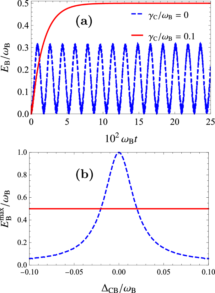
a Transient dynamics of the average energy E_B(t) of the battery in the weak driving regime F/g = 0.1 for the detuned charger-battery case with Δ_CB = 0.03ω_B. b Maximum value of the oscillating energy, ({E}_{{rm{B}}}^{max }), in the closed case (blue dashed line) is compared to the case with dephasing (red line) as function of the charger-battery detuning. Other parameter values are g = ω_B and ω_d = ω_B.

Full size image

Evidently, in the closed case since the drive-charger detuning Δ_Cd is taken equal to the battery-charger detuning Δ_CB (i.e., ω_d = ω_B), the maximum value of the oscillating energy of the battery has a Lorentzian behavior centered at Δ_CB = Δ_Cd = 0 stemming from the reduced polarization of the charger qubit and consequently suppressed energy transfer to the battery when the driving is detuned. In contrast, as shown in Fig. 4b, for the dephased charger the steady-state value of the energy is independent of detuning and becomes greater than the closed case for a wide range of detuning values away from resonance Δ_CB = Δ_Cd = 0. Since dephasing can be thought of as arising from the addition of frequency noise to the charger system (see Supplementary Section I of the SM), the charger has some frequency ‘uncertainty’ or frequency linewidth. This helps it overcome the strict detuning with the battery frequency and enables better transfer of energy than the closed case. Further details, including similar behavior for the ergotropy at weak driving as well as cases with charger driving detuned from the battery are presented in the SM (Supplementary Section II).

In summary, we have demonstrated the advantages of a dephased charger setup for the TLS battery. Our result provides a strategy for the most advantageous way to charge a TLS battery with a charger. To that end, we have to first take the ratio between the driving and coupling strength F/g = 0.5 to obtain the largest steady-state ergotropy of ({{mathcal{E}}}_{{rm{B}}}(tto infty )=0.25{omega }_{{rm{B}}}). To obtain the fastest charging time, notice from Fig. 3c that the optimal dephasing for the moderate driving regime of F/g = 0.5 is given by ({gamma }_{{rm{C}}}^{star }approx 1.15{omega }_{{rm{B}}}=2.3F). Since the charging time scales inversely with ({gamma }_{{rm{C}}}^{star }), we can further get the fastest charging by applying the optimum dephasing ({gamma }_{{rm{C}}}^{star }) with the largest allowed value of F in the particular physical realization. While we have discussed the two-TLS setup extensively here, as shown in the Methods section (see also Supplementary Sections III and IV of the SM), our central result is readily demonstrable for the two-HO and TLS-HO setups, underscoring its wide applicability. In our discussions of battery charging performance, we have focused on the energy and ergotropy as figures of merit. Since we are interested in a dissipative charging scenario, another additional variable of importance is the von Neumann entropy of the battery. We find that in general, for all the different settings we have considered, higher accumulated entropy leads to lower ergotropy as expected. Nonetheless, the steady state ergotropy with dephasing can always be tuned to a significant value by choosing the driving strength F/g appropriately or also by collectively coupling the charger to multiple battery TLSs (see Supplementary Fig. S3 of the SM). Additionally, as we discuss in the SM (Supplementary Section II), for the two-TLS case we can also express the entropy as a simple function of the difference between the energy and ergotropy (({E}_{{rm{B}}}-{{mathcal{E}}}_{{rm{B}}})).

Quantum batteries are energy storage devices that are susceptible to environmental dissipation effects. The natural question, then, is whether one can utilize these dissipative processes to enhance the overall performance of quantum batteries. In this article, we have analyzed a general method to leverage the dephasing of the charger to get fast, stable, and robust charging of a quantum battery. Our strategy, illustrated with TLS and HO models for charger and battery, relies on subjecting the charger to an optimal amount of dephasing that provides the appropriate trade-off between coherent oscillatory dynamics of energy expected at a small dephasing rate and the slow exchange of energy expected from the quantum Zeno effect at a large dephasing rate. Since this competition between coherent exchange and dephasing can occur for a wide variety of quantum systems, our main finding that moderately dephased chargers lead to efficient charging should hold universally. Moreover, for the two-TLS charger-battery setup, the dephasing also provides robustness, in terms of charging energy and ergotropy, to detuning the driving from the charger and battery. Finally, we would like to emphasize that while the focus here has been on steady state charging, in the transient regime the battery can attain values of energy and ergotropy greater than their respective steady state values. Such transient oscillations are especially pronounced for small values of γ_C. Thus, our strategy of moderate dephasing to attain robust and fast charging to a steady state can be complemented by other approaches exploiting this transient advantage, albeit with the additional requirement of precise control in switching the charger-battery coupling.

Our theoretical findings can be readily verified in state-of-the-art quantum technology platforms. For instance, recently experimental implementations of quantum batteries have been achieved with superconducting qubits⁵⁵, NMR⁵⁶, and organic semiconductor microcavity systems³⁶. In all of these realizations, the battery and charger systems are indeed exposed to an environment that can lead to dissipation and decoherence. Moreover, a key feature needed to implement our central idea, namely the ability to control the dephasing strength, has already been demonstrated in the experimental platforms of superconducting qubits⁵⁷ and NMR systems⁵⁶. Finally, while we have considered single-component battery and charger systems here, motivated by the possibility of enhancing the steady-state ergotropy of the battery (see SM), exploring collective battery-charger systems with dephasing can be an interesting future research direction^13,56.

Energy of the TLS battery and charger

The dynamics for the moments of the TLS battery-charger system are conveniently written down by moving to an interaction picture by considering a unitary transformation ({hat{U}}_{{rm{CB}}}=exp (-i[{omega }_{{rm{C}}}{hat{sigma }}_{{rm{C}}}^{+}{hat{sigma }}_{{rm{C}}}^{-}+{omega }_{{rm{B}}}{hat{sigma }}_{{rm{B}}}^{+}{hat{sigma }}_{{rm{B}}}^{-}]t)) resulting in the following Hamiltonian

with the frequency differences Δ_CB = ω_C − ω_B and Δ_Cd = ω_C − ω_d. Since the jump operator ({hat{L}}_{{rm{C}}}={hat{sigma }}_{{rm{C}}}^{+}{hat{sigma }}_{{rm{C}}}^{-}) is invariant under this unitary, the master Eq. (1) in the interaction picture reads

with ({hat{rho }}^{{prime} }={hat{U}}_{{rm{CB}}}^{dagger }hat{rho }{hat{U}}_{{rm{CB}}}). We can write down a closed set of equations for the moments (first and second) of the TLS operators from the master Eq. (10) which read as:

and

Note that the above equations are determined purely by the ratios F/g and γ_C/g in the resonant case with Δ_Cd = Δ_CB = 0. While we have chosen g = ω_B in the results shown in Figs. 2 and 3, the results remain exactly the same for even smaller coupling g, as long as we make a proportional change in F and γ_C keeping the same ratios F/g and γ_C/g. Thus, we can also understand our results as being calculated for small values of g/ω_B. Note that taking g/ω_B to smaller values also leads to smaller values of γ_C/ω_B required to obtain the dephasing enabled charging advantage as per the scaling we described. Viewing our results as being in this regime with weak system-bath (γ_C ≪ ω_B) and charger-battery (g ≪ ω_B) coupling provides additional justification for Eq. (1) as these are precisely the conditions required in standard derivations of a local GKLS master equation⁵⁸. Choosing the density matrix at initial time as ({hat{rho }}^{{prime} }(t=0)=leftvert grightrangle {leftlangle grightvert }_{{rm{B}}}otimes leftvert grightrangle {leftlangle grightvert }_{{rm{C}}}) with ({leftvert grightrangle }_{{rm{B}}}) (({leftvert grightrangle }_{{rm{C}}})) denoting the ground state of the battery (charger), the initial conditions for the moments become:

Solving Eqs. (11) and (12) with initial conditions Eq. (13) and using Eq. (4), we can write down the exact expressions for the average energy of the battery E_B(t) as

with

f₀ = 1/2, (begin{array}{l}{f}_{1}=(1+2{F}^{2}/{g}^{2}-sqrt{1+4{F}^{2}/{g}^{2}})end{array}), and (begin{array}{l}{f}_{2}=(1+2{F}^{2}/{g}^{2}+sqrt{1+4{F}^{2}/{g}^{2}})end{array}). In a similar manner, we can also write down analytical expressions for the ergotropy (see Supplementary Section II of the SM) but the analytical expressions for the ergotropy are too cumbersome to present and do not add insight. Nonetheless, we note that results in Fig. 2 were produced by evaluating the expressions using Mathematica⁵⁹.

Analytical expressions for charging time and optimal dephasing for TLS battery-charger system

Exploiting the exact expression for the battery’s average energy, we can obtain analytic expressions for the charging time at large (γ_C ≫ g) and small dephasing (γ_C ≪ g) regimes. This will allow us to support the analytical estimates for the charging time and optimal dephasing rate ({gamma }_{{rm{C}}}^{star }) presented in the main text. Taking the small dephasing limit (γ_C ≪ g) in the exact expression of the energy, Eq. (2) that determines the charging time takes the form

where the function ϕ(F, g, γ_C, t) can be determined as follows. In the limit of γ_C ≪ g, the hyperbolic trigonometric functions determining the function χ_t(γ_C, g, f_i) in the energy expression (14) will become standard trigonometric functions. The small γ_C ≪ g approximation to χ as (tilde{chi }), i.e., ({chi }_{t}({gamma }_{{rm{C}}},g,{f}_{i})mathop{approx }limits^{{gamma }_{{rm{C}}}ll g}{tilde{chi }}_{t}({gamma }_{{rm{C}}},g,{f}_{i})) takes the form

with i = 0, 1, 2. This leads to the expression for the function ϕ,

which contains only sinusoidal oscillatory terms. As a result, from Eq. (16) it is clear that the exponential term ({e}^{-{gamma }_{{rm{C}}}tau /4}) alone determines the charging time given in Eq. (6). Note that for γ_C ≪ g the charging time is independent of F and g.

Considering now the opposite limit of γ_C ≫ {F, g}, we can make the approximations:

Substituting this into Eq. (14) and keeping terms to order (frac{1}{{gamma }_{{rm{C}}}}), we can reduce the condition (2) to

In contrast to the small dephasing limit, here we have three damping timescales and the charging time will be decided by the slowest scale among them. As we show in more detail in the SM, while for the weak driving F/g ≪ 1 regime the slowest damping scale comes from the second term (4f₁/γ_C), in the strong driving F/g ≫ 1 it is given by the first term (2g²/γ_C). Noting that in the limit of F/g ≪ 1, we have ({f}_{1}=2frac{{F}^{4}}{{g}^{4}}+O({F}^{6}/{g}^{6})), and taking the inverse of the slowest damping timescale in the two regimes immediately leads to the results presented in Eqs. (7) and (8).

Results for two-HO and hybrid TLS-HO systems

To illustrate the generality of the central result presented in the paper, namely that of moderate dephasing leading to fast charging, we present the results with two additional setups. In the first case, the charger and battery are modeled as HOs and the Hamiltonian is given by

with ({hat{a}}_{{rm{B}}}) and ({hat{a}}_{{rm{C}}}) denoting the annihilation operators for the battery and charger HO, respectively. The dephasing operator in Eq. (1) is given by ({hat{L}}_{{rm{C}}}={hat{a}}_{{rm{C}}}^{dagger }{hat{a}}_{{rm{C}}}). While we present a detailed analysis of the dynamics of this setup in Supplementary Section III of the SM, Fig. 5 illustrates how moderate dephasing of the charger HO leads to fast charging for the same parameters as the two-TLS case presented in Fig. 2. Finally, we consider a hybrid setting with a TLS charger and a HO battery with the Hamiltonian

and the dephasing operator ({hat{L}}_{{rm{C}}}={hat{sigma }}_{{rm{C}}}^{+}{hat{sigma }}_{{rm{C}}}^{-}). Figure 6 illustrates our central result of dephasing enabled fast charging for this setup with a moderate driving F/g = 0.5. Similar results also hold for strong and weak driving (see Supplementary Section IV of the SM).

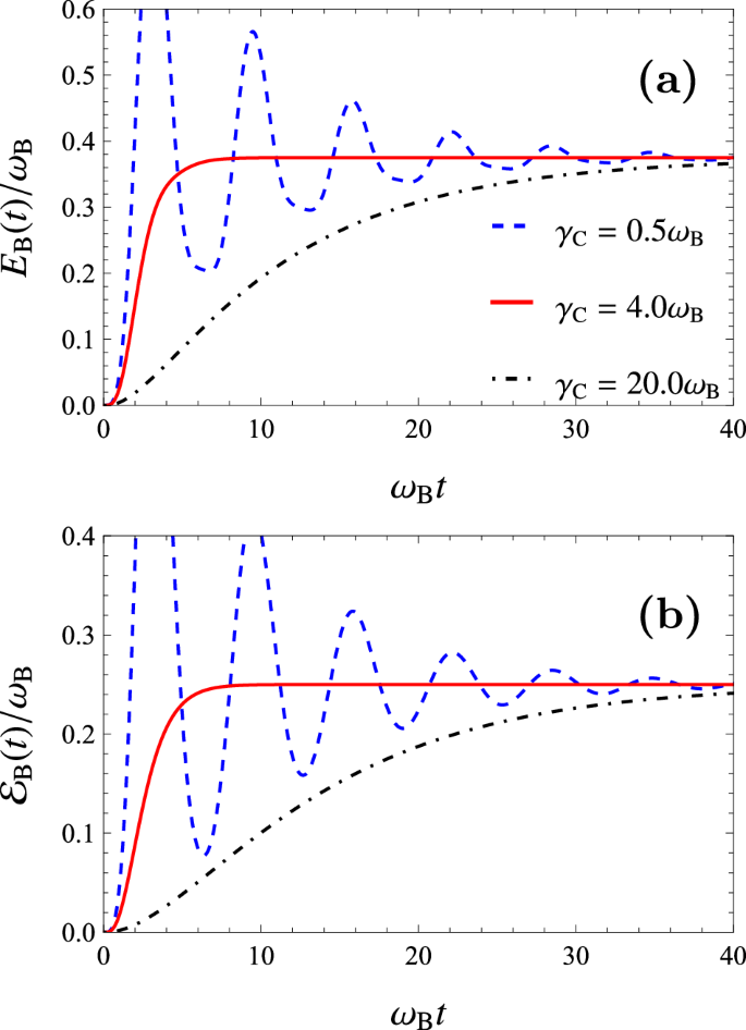
Time evolution of average energy E_B(t) (a) and ergotropy ({{mathcal{E}}}_{{rm{B}}}(t)) (b) of the battery for the two-HO model for different values of the dephasing rate γ_C. We show the resonant case, i.e. ω_C = ω_d = ω_B, for the optimal driving with F = 0.5ω_B, and g = 1.0ω_B (F/g = 0.5).

Full size image

Time evolution of average energy E_B(t) (a) and ergotropy ({{mathcal{E}}}_{{rm{B}}}(t)) (b) of the battery for the TLS (charger)-HO (battery) model for different values of the dephasing rate γ_C. We show the resonant case, i.e. ω_C = ω_d = ω_B, for the optimal driving with F = 0.5ω_B, and g = 1.0ω_B (F/g = 0.5).

Full size image

Supplementary information

In the supplementary material we provide the details regarding the derivation of the GKLS master equation, analytical calculations and dynamics with detuning for the TLS battery-charger setup, and additional details of the results with HO and hybrid TLS-HO setups. It also includes refs. ^{28,44,53,54,60,61,62,63}.