Diffraction minima resolve point scatterers at few hundredths of the wavelength

Main
A prominent question in physics is how small the distance d between two simultaneously scattering point sources can be so that they can still be distinguished using (optical) waves of wavelength λ. Identifying inelastic scatterers and measuring their distance is important in many fields, in particular fluorescence microscopy, which is the most popular imaging modality in the life sciences. Fluorescent molecules (fluorophores) can be regarded as inelastic scatterers because they dissipate a part of the illumination photon energy before emission and annihilate any phase information of the incoming light. The textbook answer is the Rayleigh limit1,2 which states that the distance between the diffraction maxima of the scatterers in an image should be larger than d = 0.61λ/(nsinα), where n and α denote the refractive index of the immersion medium and the half-aperture angle of the lens, respectively. Although it was introduced for widefield microscopy, Rayleigh’s limit also applies to scanning optical microscopy, where the object is scanned with a focused beam and the image is given by the number of photons per scanning position3.
Fluorescence microscopy does not map out the molecules of interest per se, such as the proteins in a cell, but the fluorescent markers that are linked to those molecules as labels. Although disadvantageous at first glance, this aspect is critical in superresolution fluorescence microscopy because these methods manipulate fluorophore states to obtain subdiffraction resolution. Specifically, fluorophores that reside closer than the diffraction barrier are discerned by transiently transferring a fraction of them into a fluorescent state (ON), whereas the remaining fraction is kept in a state that is dark (OFF). Placing fluorophores in different states for a brief period of detection provides separability, rendering separation by focusing obsolete4,5. This ON/OFF state transition is the key to all fluorescence nanoscopy methods known to date, including those called STED, PALM/STORM, and the more recent MINFLUX nanoscopy6 and DNA-PAINT7. Without it, none of them could provide subdiffraction resolution.
Unfortunately, the separation by ON/OFF states comes with limitations that preclude extending superresolution to other types of scattering such as Raman, let alone non-optical approaches. Even within fluorescence microscopy, the ON/OFF principle comes with a major limitation: neighbouring fluorophores are recorded sequentially. This drawback is intolerable if all fluorophores need to be observed simultaneously, as in molecular tracking. Hence, motivated by both fundamental and practical reasons, and the recent success of MINFLUX localization of ON/OFF-switching fluorophores6, we decided to reinvestigate the ability of optical microscopy to resolve scatterers that signal throughout the observation process, that is, are always ON.
Here, we show that scanning with a focused light field having a (central) diffraction minimum—rather than a maximum—allows us to identify and measure the distances between a known number of identical fluorophores down to single-digit nanometres. By colocalizing two fluorophores located only 8 nm (λ/80) apart, we show that Rayleigh’s criterion grossly overestimates the minimal distance at which two scatterers can be resolved. Thus, continuous tracking of two or more fluorophores at nanometre distances becomes viable. We also show that, for a given signal-to-noise ratio (SNR) and background, the separation precision increases with decreasing distance between the scatterers. This arguably surprising outcome also allows us to extend the method to a larger number of scatterers, which holds potential for observing nanometre conformational changes of individual proteins and other (bio)molecules with light.
Results and discussion
The diffraction maxima representing two fluorophores located at distance d < λ/2 overlap considerably in a microscopy image. This holds both for those formed by diffracted fluorescence on a camera and for the maxima gained by scanning a focused excitation beam across the focal plane and registering the emitted photons with a confocal point detector. In any case, the identification of each fluorophore is contingent upon photon noise, which is usually Poissonian (Fig. 1a,b). If the SNR is infinite and the point-spread-function (PSF) of the imaging system is perfectly known, then the fluorophores can always be resolved by deconvolution with the PSF. In practice, however, the knowledge about the PSF is limited and the SNR is too low8,9.

a, When probed with a diffraction maximum of focused illumination light of certain full-width at half-maximum (FWHM), two closely spaced scatterers (illustrated as stars) cannot be resolved for separations below the diffraction limit of (dapprox 1,{rm{FWHM}}approx 280,{rm{nm}}). For separations below this limit, changing the positions of the scatterers only marginally alters the combined scattered signal (note the similarity of the difference images for two separation values ({d}_{1}=0.03) FWHM and ({d}_{2}=0.3) FWHM shown in the panel row below). For each image, (N={10}^{6}) detected photons are considered in the calculation. b, When probed with a minimum, the same disparity in d notably alters the joint signal; note the signal increase (blue shading) in the pertinent difference images. c, One-dimensional (1D) intensity profile of scattered light when illuminating the scatterers with a diffraction maximum. Changing d yields an intensity modulation of the joint signal that remains within the noise band (standard deviation of the Poisson process) of the mean signal for both d: that is, the two sources cannot be resolved amid noise. d, When illuminating the same scatterers with a diffraction minimum, the modulation at the minimum of the resulting signal is outside the noise bands (standard deviation of the Poisson process), allowing separation. Decreasing d results in a deeper minimum of the joint signal. The insets in c and d show the profile of the individual average intensity profiles scattered by each point scatterer as well as their joint signal.
We considered the usual case where the scattered signal is proportional to the illumination intensity. Changing d between two inelastic point scatterers modulates the amplitude and spatial distribution of their joint signal I(d). For overlapping diffraction maxima (Fig. 1c), their noise adds up and the modulation is noticeable only for about (dge lambda /2). Fortunately, the modulation is easier to detect when (I(d)) is contrasted with a zero-signal baseline. Therefore, we investigated the scanning of an excitation beam with a focal intensity distribution having a central point of zero intensity. When the zero-intensity point overlapped with one of the fluorophores, we obtained zero signal from that fluorophore (Fig. 1b). At the same time, the other fluorophore exhibited fluorescence, depending on its distance to the first molecule. In fact, scanning over two scatterers with (d < lambda / 2) also yielded an (I(d)) with a single minimum (Fig. 1d), but this minimum vanished to zero only for (d=0). Hence, unless there was background, any non-zero value of the minimum indicated a finite d.
We first considered a sinusoidal excitation (fringe) pattern that was scanned over two fluorophores at distance d over a full period along the x axis (Fig. 1d). The joint signal is given by (Ileft(d,{phi }right)=) ({a}_{0}+{a}_{1}left({d}right)cos left({phi }-{{phi }}_{0}right)), where ({a}_{0}) denotes an offset and ({a}_{1}) is an amplitude varying with d. The parameter ({{phi }}_{0}) gives the phase difference of the joint signal with respect to the phase ({phi }=4uppi {x}/lambda) of the sinusoidal illumination pattern. The values of ({a}_{0}) and ({a}_{1}) depend on the brightness of the fluorophores, their separation, background and the (finite) fringe contrast of the illumination (Supplementary Information). We also introduce the modulation visibility (nu left({d}right)={a}_{1}left({d}right)/{a}_{0}).
A finite d caused the sinusoidal signals of the individual fluorophores to be shifted with respect to each other, which changed the visibility (nu left({d}right)). In contrast with the case of separation by maxima, reducing d increased (nu left({d}right)), which implies that measuring d with minima actually excels at small d. Because for (d=0) and zero background the joint signal was equal to zero, even tiny d can be measured owing to the intrinsically low noise at the minimum. By contrast, for overlapping maxima at (d=lambda /4), (nu left({d}right)) approached zero and the separation was maximally challenged by maximal values of noise. In any case, sampling (Ileft(d,{phi }right)) at three positions sufficed to determine ({a}_{0},,{a}_{1}) and ({{phi }}_{0}) and to resolve the two fluorophores at d (Supplementary Information).
A lower bound on the precision with which the position of the two emitters can be estimated is provided by the Cramer–Rao bound (CRB)10 which is directly related to the Fisher information (FI). The FI provides a measure of how much information can be inferred about the parameters of a model for (Ileft(d,{phi }right)), including the position of the fluorophores, given a statistical sample of their signal and an (Ileft(d,{phi }right)) model. We regard our signal as an inhomogeneous Poisson process with an underlying mean specified by the convolution of the illumination pattern with the sample density.
For a Poisson process, the FI is proportional to the ratio of the model gradient (squared) (nabla Ileft(d,{phi }right)) and the absolute model value (Ileft(d,{phi }right)), maximizing the FI for photons scattered from the minimum. For two sources with separation d, the CRB as the precision σ of the distance estimate scales approximately as (sigma propto frac{d}{sqrt{N}}) for the minimum and (sigma propto frac{1}{dsqrt{N}}) for the maximum. Consequently, we obtained a constant relative error σ⁄d of the estimate of d for the minimum, but a diverging relative error at small distances for the maximum (Fig. 2a). This holds true in the limit of an infinitesimally small scanning interval (Lto 0) and perfect contrast ({nu }_{0}=1) of the illumination pattern. A larger (finite) scanning range (L > 0) and an imperfect initial contrast ({nu }_{0} < 1) degraded the quality of the estimate (Fig. 2a–c). However, the estimate of d provided by a minimum was at least 100 times more precise compared with that afforded by a maximum (Fig. 2a). We note that this finding is irrespective of the shape of (Ileft(d,{phi }right)) because the decisive element is the minimum of the illumination beam, which, in first approximation, has a quadratic parabolic profile.
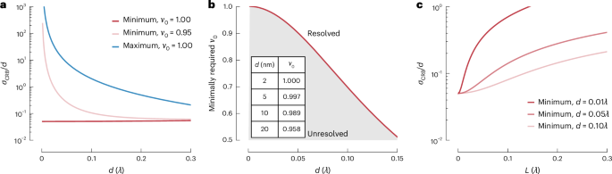
a, CRB divided by separation d, that is, relative CRB (({sigma }_{{rm{CRB}}}/d)), for different initial visibilities ({nu }_{0}). When probing with a minimum, the relative CRB for the resolution remains constant, whereas it diverges for the maximum. Imperfect contrast of the minimum of the illumination light (({nu }_{0}) = 0.95) deteriorates the precision, but the relative CRB is improved by roughly two orders of magnitude over its counterpart employing a maximum. b, Impact of the visibility ({nu }_{0}) on the resolvable distance d. Measuring small distances requires a high contrast of the illumination pattern, that is, a minimum with sufficient ‘depth’. Here, a successful distance measurement (‘resolved’) is required to exhibit a relative ({rm{CRB}}, < 0.5). The inset table provides exemplar values of required minimum visibility to measure d; here, (lambda) = 640 nm. c, Relative CRB with respect to scanning range L (in units of (lambda)) near the minimum of the combined signal, exemplified for various d. The precision improves with decreasing L, which implies that probing as close to the minimum of the joint signal improves the distance estimate.
The CRB does not guarantee the existence of an estimator that attains this precision bound. However, among a range of options (Supplementary Information), we found that a polynomial maximum likelihood estimator of the parameters ({a}_{0},) ({a}_{1}) and ({{phi }}_{0}) was sufficient to retrieve a d estimate from the photons near the minimum with a constant relative error. This advantage also remained amid non-negligible background and non-vanishing intensities at the illumination diffraction minima (Fig. 2b and Supplementary Information).
To measure the minimal distance at which two inelastic scatterers can be distinguished, we placed two fluorophores (Atto647N) at controlled distances 6 nm (< d < ,90) nm that were not resolvable at the given noise level. This sample was realized by attaching the fluorophores to a DNA origami, a so-called nanoruler11, serving as a scaffold for realizing d. Next, we employed a line-shaped interference pattern in a confocal microscope, obtained by illuminating opposing halves of the entrance pupil of a 1.4 numerical aperture oil immersion lens with two interfering 640 nm beams (Fig. 3a). Initially used for fluorophore tracking12, the line-shaped focal interference pattern of this MINFLUX set-up was oriented either in the x direction or the y direction and could be quickly interchanged by changing the x orientation and y orientation of the two beams using an electro-optical device (Fig. 3b). Destructive and constructive interference at the focal point provided a central line-shaped minimum and maximum, respectively. Changing the phase difference between the beams scanned the pattern along the x axis or the y axis (Fig. 3c) so that we could contrast the separation provided by the minimum with that by the maximum. The line scans were repeated for both the x axis and the y axis until both molecules bleached. The stack of all x or y line scans constituted an x trace or a y trace, respectively (Fig. 3d). Each trace allowed us to consider all photons or just those originating near the minimum. For both cases, we determined a projection of the distance between the fluorophores to each axis and calculated d. In addition, we recorded the sudden bleaching of individual fluorophores (Fig. 3e) so that the ensuing shift of the signal centre of mass (COM) allowed us to extract d as well (Fig. 3f–i). Pioneered in camera-based single-molecule localization13, this ON/OFF-based separation provided an independent control.

a, Scanning fluorescence microscope with photon-counting detection (APD) of fluorescence passing the dichroic mirror (DM) and a confocal pinhole (PH). The interference of two beams with adjustable phase difference (phi) entering the pupil of the objective lens creates an illumination intensity pattern in the focal plane featuring x orientated or y oriented line-shaped diffraction minima and maxima (MINFLUX set-up). Two fluorophores are sketched as stars. b, Changing (phi) scans the line-shaped minima in the x direction and y direction. c, Top: line-scan principle: linear ramp of (phi) over (2uppi) shifts the minimum across the scatterers, producing a sinusoidal line profile of fluorescence (or scattered signal). Bottom: the continuous line scan is adequately replaced by probing three points near the scatterers with the minimum (MINFLUX recording). d, Normalized counts measured during repeated line scans. The absolute number of counts decreases over time in a stepwise manner as individual fluorophores bleach. Repeated ramping of (phi) over (2uppi) in the x direction and the y direction across the scatterers yields a line-scan stack. e, Averaged counts per line, normalized over the whole stack. Two bleaching steps are clearly visible, marking transitions from two emitting molecules to one and to zero (background). f, Exemplar lines from two molecules and a single emitting molecule show the sinusoidal profile of the fluorescence counts and the spatial COM shift after the first bleaching step. Each line allowed us to extract information based on the photons just near the minimum, just near the maximum or from the entire line. g, Heat map of localizations of the fluorescence COM for two fluorophores at 20 nm distance. Inset: two clusters of localizations are visible showing the COM shift after one fluorophore was bleached. h, Averaged counts per three points MINFLUX measurement for x axis and y axis normalized over the whole measurement. The bleaching steps and fluctuations in fluorophore brightness are clearly visible. i, Normalized counts for each segment. A second order polynomial fit shows a change of the shape of the parabola after the bleaching step as well as a shift of the position of the minimum. Measurement of d relies only on photons from the first (two molecule) segment; the bleaching steps are considered just for an independent control of measured d.
Source Data
We found that scanning the entire interference pattern over the sample rendered separation inaccurate for d < 30 nm at the given noise levels, whereas selecting photons from a region just near the minimum of a trace resolved the fluorophores down to d = 10 nm. Moreover, the results nicely agree with those from the bleaching control experiment (Extended Data Fig. 1). In accordance with theory, the photons from the minimum excel at resolving at small d. Using additional photons from outside the minimum not only consumes the fluorescence budget and time, but also compromises resolution.
Consequently, we probed the fluorophores just with the excitation minimum. As in previous MINFLUX recordings12, we sampled three positions at ({x}_{-}={x}_{{rm{COM}}}-frac{L}{2},,{x}_{0}={x}_{{rm{COM}}},,{x}_{+}={x}_{{rm{COM}}}+frac{L}{2}) in each axis, whereby the size of L was iteratively reduced. The COM (({x}_{{rm{COM}}})) of the two fluorophores was subsequently estimated using the fluorescence minimum. To estimate d, a number of such triples of positions and counts was combined into a bin of a certain photon number. This procedure allowed us to reach single-digit nanometre accuracy for the d estimate with ~5,000 photons (Fig. 4 and Extended Data Fig. 2). In addition, it paves the way to resolving in dynamic settings, in which distance and location of two fluorophores have to be determined continually.
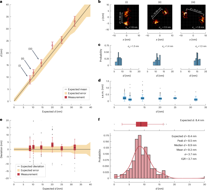
a, Measured distances d with respect to the expected distance (black line as specified by the manufacturer of the DNA nanoruler scaffold). Recording the photons originating near the illumination minimum suffices to separate simultaneously emitting fluorophores down to d = 8.4 nm within the uncertainty specified by the manufacturer (yellow shaded area). Circles indicate the medians of distances; error bars indicate twice the median absolute deviation from the median. Number of independent distance measurements per size of nanoruler (nm) are 8.4: 3,465, 10.2: 2,386, 14.3: 2,016, 20.1: 3,382, 25.0: 380, 31.8: 442. b, Exemplar localizations of two fluorophores attached to individual nanorulers with expected distances 8.4 nm (i), 10.4 nm (ii) and 14.8 nm (iii). The mean distance (d) as well as the average single-molecule localization precision (standard deviation of localizations) ({sigma }_{x,y}) is indicated. c, Corresponding histograms of the distance estimates. The standard deviation is indicated for each nanoruler. d, Box plot of obtained standard error of the mean (s.e.m.) for all nanorulers. The box extends from the lower to the upper quartile values of the data. Error bars mark the interval from the median (black line within box) to the last point within 1.5 × interquartile range (1.5 IQR). Outliers are shown as black dots. The median standard error of the mean is below 0.5 nm for all investigated systems and the 1.5 IQR is always <1 nm. Number of independent measurements are as in a. e, Box plot of the deviations from the expected distances. Number of independent measurements are as specified in a. The box extends from the lower to the upper quartile values of the data. Error bars mark the interval from the median (black line within box) to the last point within 1.5 IQR. Outliers are shown as black dots. f, Histogram of the distances obtained for the 8.4 nm fluorophore separation overlaid with the scaled probability density function (red line). The corresponding box plot from e is shown above. Comparing the total spread of the obtained deviations and the vastly different means of individual nanorulers within a batch indicates that the total spread may be partitioned into low measurement uncertainty and high production variability of the nanorulers (Extended Data Fig. 2 and Extended Data Table 1).
Source Data
To track two moving fluorophores, we translated the sample stage on a defined trajectory. Attached to a nanoruler, each of the fluorophores produced a slightly shifted copy of the trajectory of their counterpart. The distance between the fluorophores was extracted by tracking their COM and evaluating the signal for given time points. Distance estimates for fluorophores at d = 30 nm (moving along a circle with 30 nm of diameter) and at d = 15 nm (moving on a higher-order Lissajous trajectory with 15 nm amplitude) were readily obtained (Fig. 5 and Supplementary Video). Clearly not obtainable with camera-based tracking, these results demonstrate time-resolved distance measurement of identical and constantly emitting fluorophores far below the diffraction barrier. This finding also relaxes the requirements on the fluorophores, as non-switchable and non-blinking fluorophores can be used that generally bring about higher emission rates and budgets. Moreover, individual copies of such fluorophores vary much less in emission, which improves the precision of the distance estimates. Also, the usefulness of ON/OFF-switchable fluorophores in biolabelling is limited because they tend to be hydrophobic. Thus, the wide range of stable hydrophilic dyes is opened for nanoscale investigations.

a, Schematic of the measurement. A nanoruler with two fluorophores was moved on a predefined trajectory (circle) using the microscope stage. The COM of the two fluorophores was tracked with an illumination intensity minimum (dashed red line). Distances ({d}_{2}) were estimated in a bootstrapping approach along the obtained traces. b, The subsequent positions of the fluorophores were calculated relative to the current COM coordinate. This resulted in the trajectories of the individual fluorophores (two yellow circles). c, Exemplar trace of a ({d}_{2}=32) nm nanoruler moving along a circle with ({d}_{1}=30) nm diameter. Time-averaged image of the two fluorophores resulted in two displaced circles. d, Nanoruler with ({d}_{2}=15) nm moving along a Lissajous figure with amplitudes 15 nm and 20 nm in x direction and y direction, respectively. e, The trajectories of the individual fluorophores resulted in shifted copies of the COM movement. f, Exemplar trace of a ({d}_{2}=15) nm nanoruler moving along the Lissajous figure. Time-averaged image of the two fluorophores resulted in two displaced copies of the Lissajous figure. g, Time series of measured distances (thick line). The signal was obtained as a moving mean (36 ms window) on the raw data. Error bands correspond to a moving standard deviation (120 ms window). For each bin, we selected the respective tuples according to their time stamp and estimated the distance and orientation of the fluorophores. h, Histogram of measured distances (no averaging) yielded clearly distinguishable populations for nanorulers of (d=,32,{rm{nm}}) (red) and (d=15,{rm{nm}}) (blue). The histograms are overlaid with the scaled probability density function.
Source Data
As a next step, we investigated whether scanning with a minimum can also identify the position of three or more identical scatterers located in a given constellation and distance (lllambda /2). Hence, we performed measurements with three and four fluorophores arranged on DNA scaffolds either in a line, a triangle or a square. We recovered the expected scaling parameters, such as the length of the edges and distances of the nearest fluorophores (Fig. 6a–f), ranging around 20 nm.

a, Experimental localization of four emitters arranged in a square with 22 nm edge length. b, Three emitters arranged along a line with next neighbour distance 18 nm. c, Three emitters arranged in a triangular shape with 18 nm edge length. Individual fluorophores are clearly distinguishable. d–f, Histograms of all pairwise distances between localizations of individual fluorophores for a square (d), line (e) and triangular arrangement (f). Histograms are overlayed with a Gaussian mixture model fitted to the data. Histograms exhibit either a single mode, as in the case of the triangle, or two modes, as for the square and the line. For the square, the expected modes are d and (dsqrt{2}), whereas the expected modes for the line are d and 2d. Obtained mean distances of the components of the Gaussian mixture model are indicated in the respective panels. g, Numerical simulation. Spatial arrangement of up to m = 5 point scatterers (fluorophores): lines and regular polygon. The scaling parameter d denotes the nearest-neighbour distance between point sources on a line or, in the case of the polygon, the diameter of the circle circumscribing all sources. h, Numerical simulation of the relative distance error (sigma /d={rm{r.m.s.e.}}(leftlangle drightrangle )/d) for the arrangements shown in g (same colour coding). Note that at distances (d < 0.018{lambda }), five scatters in a line could be resolved more precisely than two, which indicates that the resolution favourably depends on the number of scatterers as long as the ensemble does not substantially extend beyond the minimum ((d > 0.02lambda)) of the probing intensity beam (compare the black and yellow lines). In the case of the polygon, adding a scatterer increased the emitter density: that is, it did not change the spatial extent of the ensemble, and hence improved the accuracy of the d estimate at small (d) (compare the red and blue lines). Again, this implies that, over small distances d, for example (d < ,20) nm, localization and measurement of distance between a larger number of scatterers is advantageous over a smaller number. The numerical distance values were obtained for (N=500) detected photons, a realistic probing range of (L=30) nm, an average background emission equivalent to (beta =0.1) emitting molecules in the background and λ = 640 nm.
Source Data
To explore the generality of our concept and not be limited by available samples, we also simulated other constellations of equally bright fluorophores (Fig. 6g,h). The arrangements were parametrized by a single scaling parameter d. For a linear arrangement of scatterers, d corresponded to a nearest-neighbour distance. Alternatively, d was the diameter of the circle circumscribing m scatterers forming a regular polygon. We found that the advantageous scaling of the relative error (sigma /d={rm{r.m.s.e.}}(d)/d), where r.m.s.e. is the root mean square error, remains valid for more than two scatterers. Conceptually, a smaller distance parameter d allowed us to discern a larger number of scatterers. In practice, the precision was lower bounded by experimental imperfections such as finite background, variation of brightness of individual point scatterers and reduced initial contrast of the illumination pattern, that is, a non-zero intensity minimum. Nevertheless, our results show that, for (dll lambda / 2) and commonly encountered SNR, the position of individual inelastic scatterers can be identified for various geometries. For scatterers arranged along a line at a given recurring distance d, the relative error increases with d as the ensemble substantially extends into areas of larger intensity outside the probing minimum. Interestingly, not only linear but also polygonal or grid-like arrangements of a known number of identical scatterers yield their mutual distance with a given number of detected photons.
Altogether, employing scanning diffraction minima allows, in principle, diffraction-unlimited separation of two or more constantly identical incoherent point scatterers, even at finite photon numbers. At scales of a small fraction of the wavelength, scanning MINFLUX nanoscopy does not require ON/OFF transitions for molecular separation. We have shown that this concept is applicable to scenarios involving a known quantity of scatterers constrained within subdiffraction zones at distances d ≪ λ/2, given that the general geometry of the configuration is largely understood. As the structure of many proteins is known by now from X-ray crystallography, nuclear magnetic resonance, cryo-electron microscopy or computational predictions, and as labelling with stable fluorophores is now possible at multiple protein sites, MINFLUX thus presents astonishing opportunities for probing (re)arrangements of proteins. In fact, our method has the potential to quantify the inner mechanics of single proteins using focused light.
The physical reason for this outcome is that scanning an illumination minimum across point scatterers at distance <<λ/2 automatically modulates the signal of each scatterer, so that separation is possible without modulation by a state transition. This modulation is easily detectable because it is expressed in a minimum of the scattered signal, where Poissonian noise levels are inherently low. As the modulation vanishes for larger distances, d > λ/4, our method excels only at small subdiffraction scales, which, for light, happens to be at the size of individual macromolecules (1–50 nm).
Because MINFLUX scanning exclusively relies on the interaction of the patterned illumination light with the scatterer, only their absorption matters; emission is irrelevant. For example, it is irrelevant from which fluorophore a photon actually originated. Energy transfer between fluorophores, frequently occurring at distances <10 nm, does not affect our results, adding to the reasons why our concept is so powerful at nanometre distances. By contrast, in popular camera-based superresolution methods, energy transfer between fluorophores leads to a position misrepresentation. Another aspect is that the spatial intensity profile near the minimum is always parabolic. Hence, aberrations are more easily identified. In comparison, deconvolution approaches employing maxima need to identify PSF aberrations amid large shot noise.
Owing to the wide acceptance of the Rayleigh criterion, the ability of resolving individual point scatterers with propagating waves has been underestimated. We think that this is partially due to the fact that, when employing diffraction maxima, separation becomes increasingly harder with decreasing d, rendering the idea of extracting (dll lambda / 2) futile. However, measuring with a diffraction minimum, as in MINFLUX, instantly opens up a resolution window in the (dll lambda / 2) range, identifying distances between point scatterers down to 1/80 of the wavelength and possibly even smaller in the future.
As there is no fundamental difference between fluorescence and other types of inelastic optical scattering, for example Raman scattering, our results should also be transferable to these important fields of optics. It has also not escaped our attention that our principle should also be applicable to elastic scatterers at small distances, where distance-dependent phase differences between the light scattered by different sources should be negligible. Equally intriguing is the fact that, by avoiding state transitions of the investigated material, our separation with a diffraction minimum should be applicable to any type of point scatterers of any type of propagating wave from microwaves to X-rays or even sound waves, which thus opens up superresolution to many other wave-based imaging modalities.
Methods
Experiments
The measurements were performed on a previously described set-up12 using the interference between two horizontally or vertically displaced laser beams generating an excitation beam profile with a line-shaped minimum oriented in either the x direction or the y direction in the focal plane. This minimum could be moved in the focal plane along the axis of beam separation by electro-optically changing the phase difference between the two beams.
Line-scan measurements
After a coarse prelocalization step of the COM of the linear nanoruler featuring a fluorophore at each end, the illumination pattern was alternately scanned over the nanoruler in the x direction and the y direction. When changing the phase difference linearly, and thus linearly moving the line-shaped minimum across the focal region, the emitter was subjected to a sin2 intensity modulation referred to as ‘line scan’. A full period (320 nm) of the harmonic signal was recorded, and discretized by 160 pixels and a dwell time per pixel of 500 µs. The procedure was repeated 300 times (total scan time of 48 s) at the same position until both molecules bleached. The stack of all 1D line scans of the x axis and the y axis formed the x trace and y trace, respectively. Owing to the short acquisition time, the measurement was not particularly stabilized against mechanical or thermal drift. The laser power during the phase scans was set to 20 µW, which resulted in an average count rate around 70 kHz.
Nanoruler selection
To record individual nanorulers, a 10 × 10 µm2 field of view was scanned with an average continuous-wave laser power of 2 µW. After smoothing the image with a Gaussian kernel, the spots were iteratively selected by fitting a region around the brightest pixel with a Gaussian, subtracting the fit and repeating the procedure until ten spots were found. Those spots were addressed by the galvanometer-scanner to perform the linear phase scans along the x axis or the y axis.
Line-scan analysis
Line-scan traces were composed of 1D line scans in the x axis and the y axis, which we processed independently to obtain a distance estimate in each axis and calculated the final distance as their norm. In the following, we describe the routine for an individual axis. Traces were segmented with a change point detection routine, irrespective of the count rate. (The Python package ruptures14, a piece-wise constant model and a penalized segmentation routine were used to detect a previously unknown number of change points.) The trace was split at the detected change points, and each segment was truncated five lines before and after the bleaching step. Ideally, the trace had three segments. More segments were defined depending on the number of molecules, bleaching steps or marked changes in brightness.
The traces were preselected by eye to discard obviously faulty measurements, for example, as in the case of a bright cluster of molecules or a lack of bleaching steps (only one molecule was present or the two molecules did not bleach during the measurement). Next, we automatically filtered for traces with initially two molecules, two bleaching steps and eventually zero molecules (background). Additional automatic filtering was performed on the segments to restrict the standard deviation of the average counts to less than ten times the expected Poisson noise of the mean value of the line (to filter for short blinking events). The ratio of counts between the two-molecule and the one-molecule segment was allowed to deviate by ±50%. The automatic filter routine had a success rate of 96% on the data that had been preselected by eye.
When the filtering was complete, we transited to the evaluation of the line scans. Because the selected traces had both a two-molecule and a single-molecule trace, we performed a local calibration for each phase scan by estimating the local background from the corresponding background segment of the trace and the quality of the intensity minimum (initial fringe contrast) from the single-molecule segment. This estimate served as calibration for the following evaluation of the two-molecule segment. The two-molecule segment was evaluated in a bootstrapping approach to obtain an estimate of the reduced two-molecule visibility by fitting different models to the data, for example a polynomial ansatz near the minimum or a harmonic model considering all photons of a line (see Supplementary Information for all of the available methods that we tested). The locally calibrated initial visibility and the reduced two-molecule visibility allowed us to calculate the projection of the distance in the respective axis. All analysis routines were implemented in Python.
MINFLUX measurements
We leveraged an iterative MINFLUX scanning approach, that is, scanning with intensity values around the zero point, to sample the two emitters only in a region around the minimum of the illumination pattern. In contrast with a full line scan, this drastically reduced the number of photons collected, increased the speed of the measurement and ensured the collection of the most informative photons. The actual MINFLUX routine consisted of four steps with different L values, laser powers and number of repeats. In each step, the emitter was repeatedly localized by probing at positions (left[-frac{L}{2},0,frac{L}{2}right]) around the current position estimate ({x}_{{rm{est}}}) in first the x direction and then the y direction. Each exposure lasted 158 µs which (together with waiting times for addressing new positions) resulted in a total time of around 1 ms for a complete xy localization. Based on the recorded photons, the position estimate was refined after each localization according to
where (left[{n}_{-},{n}_{0},{n}_{+}right]) represent the photons recorded at (left[-frac{L}{2},0,frac{L}{2}right]), respectively. Localizations were considered as failed if either less than five photons were collected or if (2left({n}_{+}+{n}_{-}-2{n}_{0}right) < left|{n}_{-}-{n}_{+}right|), which limited the allowed corrections to (L/2). Although the position of the COM was estimated and targeted anew after each measurement triple, the probing range L was decreased only when progressing to the next step. The first steps served to quickly localize the COM of the system (position of the minimum) and ‘zoom-in’ with the intensity minimum; only photons of the last iteration were used to estimate the separation of the source. In total, 5,000 localizations were performed resulting in a total measurement time of around 5 s. An overview over the L values, laser power and repeats is given in Supplementary Information.
Analysis of MINFLUX recordings
Measured traces consisted of tuples denoting the probing position of the illumination pattern, time and measured counts. Traces were segmented by means of a change point detection algorithm (Python ruptures). Segments were classified as background, single-molecule traces or two-molecule traces depending on the average count rate of the segment and subsequent bleaching steps before or after the segment. Segments were further treated in a bootstrapping approach to create chunks with a certain photon number, number of measurement tuples or time bins. The mode was chosen depending on the experiment. In the case of static distance measurements, a photon binning was appropriate, whereas dynamic settings required a time binning. Each chunk was fitted with various models, for example a polynomial estimator near the intensity minimum. Failed fits (those that did not converge) were excluded from further analysis.
To calibrate, we calculated the average background counts from the segments containing only background for each measurement batch (for example, size of nanorulers) and in the respective axis. This allowed calculation of the background-corrected single-molecule visibilities ({nu }_{0}) from the fit parameters of the segments containing only single-molecule data. To obtain a calibration value for each batch (size) and in each axis (x,y), we took a ({chi }^{2}) weighted median of the visibilities within each batch and axis. Note that the calibration could also have been performed in a separate measurement and that it characterized a property of the instrument. Last, we calculated the reduced visibilities on the two-molecule segments from the obtained fit parameters on the two-molecule segments. Calibrated by the background-corrected initial visibilities of the batches and in each axis, we calculated the distance projections as well as the norm for each chunk. These norms were the final distance estimates of a nanoruler with respect to the chunk identity (for example, time) and allowed a time-resolved colocalization. All analysis routines were implemented in Python.
Distance measurement by bleaching steps as a control method
Traces that contained at least one bleaching step offered an elegant way to run a control method for the distance estimate on the same data as the estimate with photons from the two-molecule segment only. Because it was unlikely that both molecules bleached at the same time, many traces contained a two-molecule segment as well as a single-molecule segment. Although the minimum of a line scan was located at the COM of the system when both molecules emitted, it jumped to the position of the remaining molecule when the other one had bleached. Hence, observing this COM shift offered an independent control for the distance estimate. By employing a polynomial model that was fitted to the minimum, we extracted the position of the minimum at any given time, averaged over the COM positions of the two-molecule trace and did the same for the single-molecule trace after the first bleaching step. The molecule distance could be estimated as twice the lateral shift of the minimum.
Stage movement for dynamic measurements
To create movements of the nanoruler and hence of the fluorophore, the stage was moved on a Lissajous curve. Therefore, the position of the stage was updated every 10 ms by adding the derivative of the desired trajectory ({mathbf{x}}_{i+1}={mathbf{x}}_{i}+Delta mathbf{x}). We assumed a Lissajous curve of the form
with amplitudes ({A}_{x,y,z}), a period of length T and potential phase shifts ({phi }_{x,y,z}) in each direction. The parameter (nu) controlled the ratio between the modulation frequencies and defined the Lissajous shape. Then, the derivative added to the current position was given by
The Lissajous parameters used in this work are given in Supplementary Information.
Numerical simulations of multi-emitter ensembles
Results for the precision of the d estimate for more than two emitters were obtained by means of a Monte Carlo simulation. We arranged emitters along a line, a regular polygon or a grid-like structure. We then simulated an iterative MINFLUX sequence resulting in a trace of tuples with positions of the illumination pattern and detected photon counts. This trace was chunked in a bootstrapping approach, conditioned to a maximum number of photons N: that is, we combined as many tuples as necessary until the sum of all collected photons reached the required value. The distance parameter d was then estimated on these chunks, and the r.m.s.e. of the estimates was calculated. The relative error was given by the fraction of the r.m.s.e. and the ground truth value of the parameter d.
Sample preparation
Cleaning process of cover slip
To clean the cover slips (170 μm, no. 1.5H, Paul Marienfeld GmbH & Co. KG) measuring 15–18 mm in width, the following procedure was carried out. Initially, they were gently wiped using a lint-free cloth sprayed with acetone. Subsequently, another cloth sprayed with isopropanol was used to wipe them. After rinsing the cover slips with isopropanol, they were dried using a nitrogen flow. Finally, a plasma cleaning process (using oxygen) was carried out for 5 min at 200 W.
Construction of flow chamber
To facilitate the easy exchange of incubation solutions during preparation and buffer changes between experiments, flow chambers were created. This involved attaching two narrow strips of double-sided tape (Scotch double-sided tape, 3M) to a microscope slide, forming a channel approximately 5 mm wide. A cleaned cover slip was then placed on top of the tape and secured by applying gentle pressure.
Preparation of nanorulers
Preparation of the DNA structures (nanorulers, GattaQuant GmbH) was carried out with the following routine (see Supplementary Information for manufacturers of the substances):
-
(1)
Clean cover slip.
-
(2)
Prepare flow channel.
-
(3)
Pipette the following through the flow channel:
-
(a)
200 μl phosphate-buffered saline (PBS) (flushing the flow channel)
-
(b)
15 μl bovine serum albumin-biotin (1:2 in PBS), wait two minutes
-
(c)
200 μl PBS (flushing the flow channel)
-
(d)
15 μl strepatvidin (1:2 in PBS), wait two minutes
-
(e)
200 μl PBS (flushing the flow channel)
-
(f)
15 μl GattaQuant rulers (diluted 1:50 or 1:100 in PBS), wait two minutes
-
(g)
600 μl PBS (flushing the flow channel)
-
(h)
15 μl buffer
-
(i)
seal edges with epoxy
-
(j)
store in fridge.
-
(a)
The buffer consisted of an imaging buffer (IB), methylviologen (MV, 75365-73-0, Sigma Aldrich) and a pyranose oxidase-based enzyme system as specified below. It was prepared by mixing 100 μl IB, 1 μl 0.2M MV and 1 μl of the enzyme system. Reagents for the IB were PBS (basis), 10% glucose (with respect to mass) and 2 mM Trolox (with respect to final concentration in IB). The enzyme system was prepared by mixing 10 mg pyranose oxidase (Pyranose Oxidase (P4234-1KU), Sigma-Aldrich Chemie GmBH), 170 μl PBS and 80 μl catalase (C100-50MG, Sigma-Aldrich Chemie GmbH). Additionally, premounted samples of nanorulers were purchased directly from GattaQuant.

Responses