Direct entanglement detection of quantum systems using machine learning

Introduction
Entanglement plays a crucial role in the development of quantum technologies1. It is an essential resource for simulating many-body physics2,3, investigating quantum advantages in quantum computation, and ensuring the security of quantum communication4,5. Unfortunately, entanglement measures are not physical observables, making detection and quantification extremely challenging6.
In the Noisy Intermediate-Scale Quantum (NISQ) era, new demands for quantum entanglement detection are being put forth. Demand 1: Quantifying entanglement effectively. Although a large number of entanglement witnesses have been constructed7,8,9, some of which only require partial system information10, they only provide a yes or no answer as to whether entanglement exists or not. Accurate quantification of entanglement, such as logarithmic negativity11 and the PT moments12,13, typically requires quantum FST since there are no observables for them. However, due to the exponential increase of the number of measurements with system size, performing FST to measure entanglement will no longer be practical for NISQ devices. In recent years, a large number of methods have been proposed to boost the efficiency of FST14,15,16,17,18,19, including compressed sensing16, FST via local measurements17,18, and neural network FST15, but these methods may not be effective for entanglement measurement since two close states may have significantly different values of entanglement20. Therefore, it is increasingly essential to develop effective entanglement measurement techniques. There have been extensive studies aimed at meeting this need21,22,23,24. The authors use random measurements to measure the second-order Rényi entropy of subsystems24. Demand 2: Detecting entanglement dynamics beyond the measurement time. Non-equilibrium quantum simulations25,26,27, such as quantum thermalization, typically require long-time dynamics, but current NISQ devices still have limited coherence times. This implies that measuring long-time entanglement will be difficult. Several studies have used neural networks to investigate the long-time dynamics of local observables beyond the measurement time28. But it remains an open question whether it is possible to predict long-time entanglement at an unseen future time based on local measurement data in an observable time window.
In this work, we propose a machine learning-assisted detection protocol to determine entanglement from local measurements and validate it by quantifying the entanglement of the ground and dynamical states of the local Hamiltonian. For dynamical states, the entanglement dynamics beyond the measurement time are also accurately predicted from the single-qubit time traces only in the previous time window. Moreover, we implement an experiment to demonstrate the feasibility of our approach. We employ it to measure static entanglement in ground states and entanglement dynamics in dynamical states of a one-dimensional spin chain on the nuclear magnetic resonance (NMR) platform, and two-local measurements provide accurate predictions of static entanglement as a function of system parameters. For the dynamical case, the entanglement dynamics beyond the measurement time are accurately estimated from the single-qubit time traces using our machine learning approach. Our machine learning approach offers a wide variety of applications in the study of quantum many-body entanglement.
Results
The protocol for entanglement detection
The characterization and measurement of quantum entanglement is a crucial task in quantum simulation2,3, which typically prepares the ground state ({mathcal{H}}vert {psi }_{g}rangle ={E}_{g}vert {psi }_{g}rangle) or realizes the dynamical state (vert psi (t)rangle =exp (-i{mathcal{H}}t)vert {psi }_{0}rangle) of a given local Hamiltonian ({mathcal{H}}=mathop{sum }nolimits_{i = 1}^{m}{c}_{i}{B}_{i}) with Pauli basis Bi. Their entanglement can be characterized by measuring the entanglement entropy and PT moment. The entanglement entropy provides information about the entanglement contained in the system. It is calculated using the equation ({{mathcal{S}}}^{(n)}=frac{1}{1-n}log (,{text{tr}},{rho }_{A}^{n})). ρA is the reduced density matrix of the total system ρAB. In particular, ({{mathcal{S}}}^{(2)}) is the second-order Rényi entropy, which has been used to study entanglement growth and thermalization. The PT moment is defined as ({{mathcal{P}}}_{n}=,text{Tr},[{({rho }_{AB}^{{T}_{A}})}^{n}]). ({rho }_{AB}^{{T}_{A}}) is a partial transpose with respect to subsystem A. ({{mathcal{P}}}_{1}=1), ({{mathcal{P}}}_{2}=,{text{Tr}},[{rho }_{AB}^{2}]), and ({{mathcal{P}}}_{3}) is the lowest PT moment that provides information about the entanglement. The first three PT moments have been used to test the bipartite entanglement29. Quantum coherence in many-body simulation embodies the essence of entanglement in the following form of ({mathcal{C}}=S({rho }_{{rm{diag}}})-S(rho ))30,31. ρdiag is the diagonal matrix obtained by removing all off-diagonal elements from ρ. The above set of entanglement quantities ({mathcal{E}}equiv {{{mathcal{S}}}^{(n)},{{mathcal{P}}}_{n},{mathcal{C}}}) commonly requires FST or multi-copy measurements.
To avoid these issues, we use machine learning to directly predict ({mathcal{E}}) from local Pauli measurements ({mathcal{O}}) on the ground state (vert {psi }_{g}rangle) or dynamical state (vert psi (t)rangle) of the local Hamiltonian ({mathcal{H}}). Figure 1 presents the principle of our neural network. The nonlinear relationship between ({mathcal{O}}) and ({mathcal{E}}) can be approximated by a multilayer neural network with a finite number of neurons. This method train a neural network with a large set of known inputs ({mathcal{O}}) and outputs ({mathcal{E}}). Once the models are trained to convergence, they can be used to experimentally predict the unknown ({mathcal{E}}) from the measured ({mathcal{O}}), without quantum FST. For the ground state, the input ({mathcal{O}}={langle {psi }_{g}vert {B}_{i}vert {psi }_{g}rangle ,1leqslant ileqslant m}) is the set of the expectation values of local Pauli operators Bi on the ground state (vert {psi }_{g}rangle) and the output is static entanglement ({mathcal{E}}) of (vert {psi }_{g}rangle). Here, a fully connected neural network (FCNN) is employed to map the relationship between input ({mathcal{O}}) and output ({mathcal{E}}). For the dynamical state, the input ({mathcal{O}}={langle {psi }_{stau }vert {sigma }_{x,y,z}^{(i)}vert {psi }_{stau }rangle ,1le sle S,1le ile N}) is the set of the expectation values of single-qubit Pauli operators of each qubit at each moment sτ. S is the number of sampling points, and τ = Ttra/S is the sampling interval. The measured data at the moment sτ is fed into the s-th long short-term memory (LSTM) cell before using FCNN to decode the data. The dynamical entanglement ({mathcal{E}}(t)) is the output result. More intriguingly, once trained, the trained model is able to predict the long-time entanglement ({mathcal{E}}(t)) in an unseen time window [Ttra, Ttot] based on the measurement ({mathcal{O}}(t)) in [0, Ttra]. This means that our neural network is able to measure the entanglement dynamics beyond the measurement time. We train the neural network using adaptive moment estimation, a well-known optimizer in machine learning. More details about our neural network can be found in Supplemental Information (see the Supplemental Material for details).

a For the ground states (vert {psi }_{g}rangle), local Pauli operators are measured and they are directly used to learn ({mathcal{E}}) via FCNN. b For the dynamical states (vert {psi }_{t}rangle), we only measure and input the expectation values of single-qubit Pauli operators in the range [0, Ttra]. It can predict not only the dynamics of ({mathcal{E}}) during the training window, but also the long-time dynamics of ({mathcal{E}}) at the unseen time [Ttra, Ttot].
Numerical results
To demonstrate the feasibility of our neural network, we first numerically test the following Hamiltonian models.
Model 1
We consider a 6-qubit two-local Hamiltonian ({mathcal{H}}=mathop{sum }nolimits_{i = 1}^{6}{{boldsymbol{omega }}}^{i}cdot {{boldsymbol{sigma }}}^{i}+mathop{sum }nolimits_{j = 1}^{5}{{boldsymbol{sigma }}}^{j}cdot {{boldsymbol{J}}}^{j}cdot {{boldsymbol{sigma }}}^{j+1}) and train a neural network to predict the static ({mathcal{E}}) of the ground states. ({{boldsymbol{sigma }}}^{i}=({sigma }_{x}^{i},{sigma }_{y}^{i},{sigma }_{z}^{i})) is the vector of Pauli matrices. ({{boldsymbol{omega }}}^{i}=({omega }_{x}^{i},{omega }_{y}^{i},{omega }_{z}^{i})) and ({{boldsymbol{J}}}^{j}=({{boldsymbol{J}}}_{xx}^{j},ldots ,{{boldsymbol{J}}}_{zz}^{j})) represent the external magnetic field strength and the coupling tensor, respectively. During training, we generate a large number of ground states (vert {psi }_{g}rangle) by randomly choosing ω, J ∈ [−1, 1], and using ({mathcal{O}}) and ({mathcal{E}}) of the ground states as input and output, respectively. ({mathcal{O}}) is the set of the expectation values of the one and two-body Pauli measurements of the state, which can be easily obtained. The predicted ({mathcal{E}}) includes the entanglement information of the subsystems. We generate 100,000 pairs of such (({mathcal{O}}), ({mathcal{E}})) for training the neural network and then randomly select 500 for testing the performance. In Fig. 2a, we compare the estimation of ({{mathcal{S}}}^{(2)}), ({{mathcal{P}}}_{3}), and ({mathcal{C}}) by our neural network with the traditional FST. To test the feasibility of our machine learning method in large systems, we employ a tensor network-based simulation approach to train our machine learning model for systems with up to 20 spins. Similarly, we consider a 20-qubit two-local Hamiltonian model,
whose parameters are in the range [−1, 1]. This Hamiltonian is modeled on nearest-neighbor interactions, which may result in localization in the presence of strong disorder (see the Supplemental Material for details). Our numerical investigations into the localization behaviors of the Hamiltonians described in Eq. (1) focused on two indicative features: energy spectrum statistics and entanglement signatures. Our findings reveal no noticeable localization when the disorder strength is below 1; however, the system tends towards a localized phase under considerably strong disorder. Specifically, the Hamiltonian induces localization only when the disorder strength exceeds 10. Detailed results of these simulations are available in the Supplemental Information (see the Supplemental Material for details). We employ tensor networks to randomly generate the ground states of 20-spin Hamiltonians for training our neural network. We use tensor network-based simulations for several reasons. Primarily, our simulations require the computation of ground states of Hamiltonians. A 20-spin Hamiltonian forms a matrix of size 220 × 220, rendering direct diagonalization impractical due to the computational intensity. In addition, we simulate the entanglement of ground states to serve as labels for the neural network, which necessitates the use of density matrices instead of state vectors. Consequently, managing a 220 × 220 density matrix is similarly impractical. So the purpose of using tensor networks is to efficiently generate training data for our machine learning model, not limited to 20 spins. The input data set contains the Pauli measurement information of the single-qubit and the nearest two-qubits, and the output data set contains the Rényi entropy of the sequential subsystems (A = 1, 12, 123, 1234, etc.) until the front 10-qubit subsystem. After successfully training the neural network for 20-spin systems, we randomly select 1000 test data set to test the performance of trained neural networks. In Fig. 3, we compared the estimation of Rényi entropy ({{mathcal{S}}}^{(2)}) of the subsystem (1–10 qubits) by our neural network with the traditional quantum state tomography. It clearly shows that our machine learning approach is able to predict the entanglement information of the ground state of the 20-spin Hamiltonian without quantum state tomography. Meanwhile, in contrast to the 410 − 1 (about one million) Pauli measurements that are required in 10-spin subsystem FST, our machine learning method only requires (20 − 1) × 9 + 20 × 3 = 231 single-qubit and the nearest two-qubit Pauli measurements.
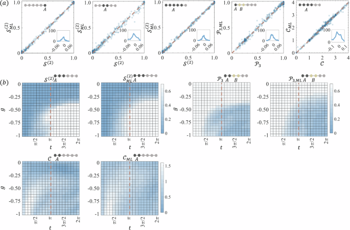
a The correlation figures between the predicted entanglement ({{mathcal{E}}}_{{rm{ML}}}) from 2-local measurements and the theoretical ({mathcal{E}}). The inset figures are the distributions of the difference ({{mathcal{E}}}_{{rm{ML}}}-{mathcal{E}}). b Prediction of entanglement dynamics ({{mathcal{E}}}_{{rm{ML}}}(t)) from single-qubit time traces. In each pair of comparisons, the right column is the prediction result obtained by our machine learning method and the left column is the theoretical values. The input layer contains only the measured single-qubit time traces in [0, π]. The trained model allows us to predict ({{mathcal{E}}}_{{rm{ML}}}(t)) at the unseen time [π, 2π]. The measured subsystems are represented by the gray rounded schematic.
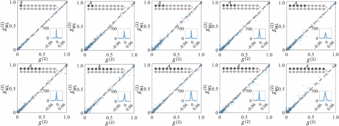
The measured subsystems are represented by the gray rounded schematic. We randomly select 1000 for testing the performance after our neural networks are trained. The inset figures are the distributions of the difference ({{mathcal{S}}}_{{rm{ML}}}^{(2)}-{mathcal{S}}).
Model 2
We train a neural network capable of predicting the entanglement dynamics of the non-equilibrium states. The system starts from (leftvert {psi }_{0}rightrangle ={R}_{z}(pi /8){R}_{y}(pi /8){leftvert 0rightrangle }^{otimes 6}) and evolves into (leftvert {psi }_{t}rightrangle =exp (-i{{mathcal{H}}}_{{rm{d}}}t)leftvert {psi }_{0}rightrangle) under the Hamiltonian ({{mathcal{H}}}_{{rm{d}}}). ({{mathcal{H}}}_{{rm{d}}}) is defined as ({{mathcal{H}}}_{{rm{d}}}=Jmathop{sum }nolimits_{i = 1}^{5}{sigma }_{z}^{i}{sigma }_{z}^{i+1}+gmathop{sum }nolimits_{j = 1}^{6}{sigma }_{x}^{i}), where J and g are adjustable parameters. ({{mathcal{H}}}_{{rm{d}}}) is one of the models used in the study of entanglement dynamics32. We generate various ({{mathcal{H}}}_{{rm{d}}}) by randomly selecting J and g between −1 to 1, allowing the initial state to evolve in various ways to a large number of (leftvert {psi }_{t}rightrangle). The neural network is trained by taking (({mathcal{O}}), ({mathcal{E}})) of each state at a time as input and output. This model differs from the previous one in that we use only single-qubit Pauli measurements. The predicted ({mathcal{E}}) includes the entanglement dynamics of the subsystems. Here, we still use 100,000 data for training the neural network, and we only feed ({mathcal{O}}) in the previous time [0, π] as the input during training. The output is the entanglement dynamics ({mathcal{E}}(t)) in a longer time range [0, 2π]. We set J = −0.5 and divide g from −1 to 0 into 20 parts to generate 20 pieces of data to test our neural network. Figure 2b depicts the predicted ({{mathcal{S}}}^{(2)}(t)), ({{mathcal{P}}}_{3}(t)), and ({mathcal{C}}(t)) for the time interval [0, 2π]. It is shown that ({mathcal{E}}(t)) can be accurately predicted from the single-qubit time traces32.
Extension to other models
More importantly, our machine learning approach can be easily extended to other Hamiltonians, including quantum l-local Hamiltonians, long-range interaction Hamiltonians, 2D Hamiltonian models, molecular systems relevant to quantum chemistry, etc. As a demonstration, we also test the application of our machine learning approach to estimating the entropy of the ground state of a long-range interaction Hamiltonian ({{mathcal{H}}}_{{rm{Long}}}) and a 2D random Heisenberg model ({{mathcal{H}}}_{2D}).
({{mathcal{H}}}_{{rm{Long}}}) is the commonly considered model, such as the works24,29. ({{mathcal{H}}}_{2D}) is a 2D anti-ferromagnetic random Heisenberg model considered in the work33. Here, we consider only n = 6 by exact diagonalization for the demonstration. The results are shown in Fig. 4a. The demonstration on larger models can be obtained using DMRG (Density Matrix Renormalization Group).
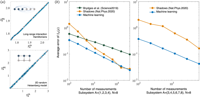
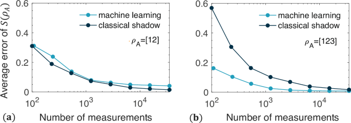
a The applications of our machine learning method in the model ({{mathcal{H}}}_{{rm{Long}}}) and ({{mathcal{H}}}_{2D}). Here, ({S}_{A}^{th}) is the real entropy of the half-length subsystem and ({S}_{A}^{ML}) is the prediction result of our machine learning. b Comparison of our machine learning method with the randomized measurement toolbox proposed by Brydges et al.24 and the classical shadows proposed by Huang et al.22 for predicting second-order entanglement entropy in 8-qubit ground states. Here, we consider the entanglement entropy of the subsystem A = {1, 2, 3, 4} and A = {3, 4, 5, 6, 7, 8}, respectively. It is well-known that machine learning methods fail to achieve 100%-accurate predictions and their accuracy is limited by the machine learning model. Thus, machine learning methods lose their advantage when the number of experiments is infinite, but in practice a finite number of experiments are scheduled.
Numerical comparison with existing methods
A detailed comparison with the existing method is presented here. First, our approach directly predicts the entropy of the subsystem without learning a prior on the classical representation of the quantum system. Current machine learning methods for quantum many-body systems typically learn a classical representation of the quantum system. However, since many measures of entanglement are not continuous, these may be insufficient for predicting entanglement. Namely, even if the learned state is very closely approximated by the actual state, the two may have significantly different values of entanglement. Our direct estimate of the entropy of the system avoids this problem. Second, our method only involves measuring the expectation values of local Pauli operators, which are commonly observed in experiments. Moreover, our approach doesn’t require ancillary qubits or complex controlled operations. There is a typical work that directly predicts entanglement via machine learning23, but it requires measurements of partially transposed moments as input, which is very difficult to implement experimentally. In fact, there are two primary challenges in implementing the technique described. First, partially transposed moments do not correspond to physical observables in experimental setups. While this study offers a solution to this issue, it requires doubling the qubit resources. Second, the technique necessitates controlled operations between two quantum copies. Both factors present substantial challenges for current quantum processors, which are constrained by limited qubit availability, circuit depth, and control accuracy. These limitations render the approach more theoretically viable than practically feasible at this stage.
In addition to machine learning methods, there are some well-known randomized methods for directly predicting the entropy of a system, mainly including the randomized measurement toolbox and classical shadows22,24. It is important to note that these methods have their own strengths and weaknesses. Both the randomized measurement toolbox and the randomized measurement toolbox work for any arbitrary states, but they require exponential measurements in the subsystem size. Our method is applicable for structured quantum states, such as the ground states and the dynamical states of quantum many-body Hamiltonians (a molecular system relevant for quantum chemistry and l-local Hamiltonians), but it only requires polynomial measurements. In this way, they form a complementary relation and are suitable for different applications in measuring the second-order Rényi entropy of subsystems, where our approach would be a better choice for structured quantum states, as it captures the central information and the classical shadows and random measurement toolbox would perform better for arbitrary states. We have performed a comparison between our method, classical shadows, and the randomized measurement toolbox for estimating the second-order Rényi entanglement entropy of subsystems in the ground states. Figure 4b shows the comparison results. The details can be found in the Supplemental Information (see the Supplemental Material for details). This clearly shows that our method requires fewer measurements and that the discrepancy will increase as we require larger sizes. In the comparison, the y-axis represents the average error, which is defined as the mean distance between the actual entropy Sth and the predicted entropy SML,RM,CS. These values are obtained through machine learning, randomized measurements, and classical shadow methods. The average error is calculated as (epsilon =frac{1}{M}mathop{sum }nolimits_{m = 1}^{M}| {S}_{m}^{{rm{th}}}({rho }_{A})-{S}_{m}^{{rm{ML,RM,CS}}}({rho }_{A})|), where M denotes the number of test samples. Besides, we define “one projection measurement” as “one experiment”. Thus, the “number of measurements” (x axis) represents the total number of projection measurements, which corresponds to the measurement cost of obtaining entropy. Machine learning methods generally follow a “train once, use repeatedly” principle. Once trained, the machine learning model can make predictions on new data without requiring further training. Therefore, the x axis in Fig. 4b excludes the training experiments.
Experimental demonstration
We also adopt our neural networks to predict static entanglement ({mathcal{E}}) and non-equilibrium entanglement dynamics ({mathcal{E}}(t)) on a 4-qubit nuclear magnetic resonance (NMR) platform34,35. The used four-qubit sample is 13C-labeled trans-crotonic acid dissolved in d6-acetone, where four 13C nuclear spins are encoded as a 4-qubit quantum processor. The internal Hamiltonian of the system is given by
νi is the chemical shift of each spin, and Jij is the coupling strength between different spins. The spin dynamics is controlled by shaped radio-frequency (rf) pulses36. The molecular structure and the Hamiltonian parameters can be found in the Supplemental Material (see the Supplemental Material for details). All experiments were carried out on a Bruker 600-MHz spectrometer at room temperature.
First, we observe ({mathcal{E}}) in two types of spin-half chains by studying the entanglement of their ground states. Their Hamiltonians are defined as
Their ground states exhibit jump across singularities characterized by sudden entanglement as a function of Δ or hz37,38. Δ is the anisotropic parameter characterizing the magnetic field. In experiments, we prepare 50 ground states by changing Δ and hz from −1 to 1 with a step of 0.04, measure the expectation values of the two-local Pauli operators, and then use our trained neural network in Model 1 to predict the entanglement information of these states. Second, we investigate the non-equilibrium phenomena by characterizing the entanglement evolution ({mathcal{E}}(t)) of the dynamical states of ({{mathcal{H}}}_{{rm{d}}}). Experimentally, we prepare the initial state (leftvert {psi }_{0}rightrangle ={R}_{z}(pi /8){R}_{y}(pi /8){leftvert 0rightrangle }^{otimes 4}) and implement the dynamical evolution of the two Hamiltonians with the parameters J = − 0.5, g = − 0.3 and J = − 0.5, g = −0.75. We then measure the single-qubit time traces and use the trained neural network to predict the entanglement dynamics ({mathcal{E}}(t)). Here we also perform quantum FST on the ground states and dynamical states to provide a comparison with machine learning results. Our experiment consists of the following steps.
-
(i)
Initialization: We first initialize the spins to a pseudo-pure state (PPS) ({leftvert 0rightrangle }^{otimes N}) from the highly mixed state via the selective-transition method39,40,41. Quantum FST was also performed to check the PPS quality. A fidelity of more than 99% provides a reliable initialization for the following experiments.
-
(ii)
Preparing target states: For the ground states of ({{mathcal{H}}}_{{rm{XX}}}) and ({{mathcal{H}}}_{{rm{XXZ}}}), we optimize a 20 ms shaped pulse to drive the system to the target states from ({leftvert 0rightrangle }^{otimes 4}). For the dynamical states of ({{mathcal{H}}}_{{rm{d}}}), we also optimize a 30 ms shaped pulse that realize the evolution (exp (-i{{mathcal{H}}}_{{rm{d}}}t)). All shaped pulses are searched with the gradient ascent pulse engineering (GRAPE) technique42.
-
(iii)
Measuring local information: We measure the expectation values of ({mathcal{O}}). It consists of 39 Pauli measurements (3 × 4 single-qubit Pauli operators {σi}, 3 × 9 two-qubit Pauli operators {σiσi+1}) for the static models ({{mathcal{H}}}_{{rm{XXZ}}}) and ({{mathcal{H}}}_{{rm{XX}}}) (see the Supplemental Material for details). For the dynamical states of ({{mathcal{H}}}_{{rm{d}}}), we measure 50 temporal points from 0 to π with a step of π/50 and measure 3 × 4 single-qubit Pauli operators {σi} each moment. As an ensemble system, NMR can easily measure the expectation value of the Pauli operators.
-
(iv)
Predicting entanglement: We first trained the neural networks with 100,000 numerical training data for both the static and dynamic models. We then feed the measured data in the above experiment step into the trained neural network to predict the entanglement of the target state.
The predictions of entanglement quantities by our neural networks display a singularity jump precisely where the theoretical way occurs. In the left of Fig. 5, we show the static entanglement obtained by theoretical calculation (solid line), quantum FST (red points), and our neural networks (blue points). In the ({{mathcal{H}}}_{{rm{XXZ}}}) model, we set J = − 0.5, and the singular point occurs when the model reverts to an isotropic Heisenberg model (Δ = J). In the ({{mathcal{H}}}_{{rm{XX}}}) model, we set J = −0.3, and we can observe the magnetic critical point where the ground state energy levels cross (({h}_{z}=2Jcos (frac{kpi }{5})), where 1≤k≤4 is an integer)37. In the right of Fig. 5, we show the dynamic nature of the entanglement ({mathcal{E}}(t)) in [0, 2π] using the measured single-qubit time traces. Different dynamic behaviors will be observed in the cases of g < gc and g >gc32. When g = −0.3, the oscillation amplitude of ({mathcal{E}}(t)) (blue line) is modest and close to its initial value, and when g = −0.75, ({mathcal{E}}(t)) (red line) oscillates range is greatly larger (see the Supplemental Material for details).
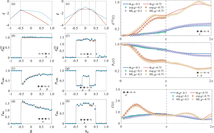
a, e are the ground energy levels (red lines). The energy levels of the first-excited state are also included (blue lines). b–d, f–h show the entanglement ({mathcal{E}}) of the ground states of ({{mathcal{H}}}_{{rm{XXZ}}}) and ({{mathcal{H}}}_{{rm{XX}}}) models, respectively. Theoretical calculation (solid lines), quantum FST (red points), and our neural network results (blue points) are distinguished. The measured subsystems are represented by the gray rounds schematic. Right plot: The dynamical evolution ({{mathcal{S}}}^{(2)}(t)) (the subsystem A = 12), ({{mathcal{P}}}_{3}(t)) (the subsystems A = 1, B = 2), and ({mathcal{C}}(t)) (the subsystem A = 12) for two sets of parameters (i) J = −0.5, g = −0.3 and (ii) J = −0.5, g = −0.75. The input layer only contains the measured single-qubit time traces in [0, π]. The trained model allows us to predict ({mathcal{E}}(t)) in the training window [0, π] and in the unseen future time window [π, 2π]. The theoretical results (solid lines), quantum FST results (square dots), and predicted results (diamond dots), for the two setups, are each represented by a different color of identification line (or dot).
Meanwhile, we also make the comparison with classical shadows using the experimental data, considering that classical shadows might be expected to allow for an arbitrary set of errors, including control and decoherence noise in the real situations. However, The classical shadow method relies on projection measurements, making it unsuitable for NMR platform, which is ensemble-based and cannot perform projection measurements. To apply the classical shadow method to the real errors encountered in NMR experimental data, we simulate projection measurements via Monte Carlo on the reconstructed density matrices from NMR, which contain the real errors. We then compare the performance of our machine learning method with classical shadows in detecting entanglement entropy across different numbers of projection measurements. Figure 6 presents the corresponding results. The results indicate that the machine learning method requires fewer measurements, especially at low sampling rates for large subsystems. This is because classical shadows need exponentially more measurements as subsystem size increases. The difference between them becomes more obvious with larger subsystems (see Fig. 4). However, classical shadows can achieve more accurate entropy estimation with sufficient measurements, as they can manage a broader range of errors. Moreover, there are significant differences between the two methods. First, the machine learning method measures the expectation values of local Pauli operators, making it compatible with all quantum processors. In contrast, classical shadows only work on platforms capable of projection measurements. Second, machine learning methods are typically “once and for all”; once the model is trained, it doesn’t need retraining, allowing for quick predictions on new measurement data. On the other hand, classical shadows require constructing quantum state representations from measurement data and then calculating entropy through summation over ({C}_{M}^{2}) terms (refer to Fig. 1 of the supplemental information for more details). M denotes the number of classical shadows.
It shows no clear advantage for ρA = [12] in a due to the small subsystem size. However, a significant advantage emerges for ρA = [123] in b. The difference becomes more obvious with larger subsystems (see Fig. 4 in the main text). Here, the average error, defined as the mean distance between the real entropy SNMR (obtained through quantum state tomography) and the predicted entropy SML,CS (obtained through machine learning and classical shadow methods), is calculated as (epsilon =frac{1}{M}mathop{sum }nolimits_{m = 1}^{M}| {S}_{m}^{{rm{NMR}}}({rho }_{A})-{S}_{m}^{{rm{ML,CS}}}({rho }_{A})|). M denotes the number of reconstructed density matrices in the experiments.
Discussion
In this section, we primarily discuss the applications of our machine learning method in practical scenarios where the Hamiltonian models may deviate from those used during training, such as instances involving unscrupulous actors generating separable states to deceive the system, or cases with rapidly oscillating entanglement dynamics. Additionally, we explore how the number of training points scales with problem size and identify specific applications where implementing our machine learning method is beneficial.
The robustness against control and decoherence noises
In real-world scenarios, the experimental models may deviate from the Hamiltonian models used during training due to factors like control noise and decoherence in current quantum processors. This issue is common in current machine learning approaches for solving quantum problems. Fortunately, noise sources in quantum systems can typically be described within a consistent mathematical framework. The quantum community has also developed robust and well-validated techniques for noise characterization43,44,45, such as Dynamical Decoupling, Randomized Benchmarking, and Gate Set Tomography. These methods enable accurate characterization of quantum noise models, which can be reliably incorporated into machine learning model training to enhance feasibility on actual quantum devices.
Here, we first analyze the robustness of the machine learning model trained on perfect Hamiltonians against these noises. We simulate the noisy test data using the following steps. Here, we consider there is a control error distribution θ = N(θg, ξ) in the parameterized quantum circuits U(θg) for preparing the perfect ground states (vert {psi }_{g}rangle) of Hamiltonians. It is (vert {psi }_{g}rangle =U({theta }_{g}){vert 0rangle }^{otimes N}). N(θg, ξ) is a Gassuian distribution with the mean value of θg and the standard deviation of ξ. We generate 500 noisy states (vert psi rangle =U(theta ){vert 0rangle }^{otimes N}) incorporating control noise and predict their entropy using the machine learning model trained on perfect Hamiltonians. Figure 7a illustrates the distance between the actual entropy of (vert psi rangle) and the predictions from the machine learning model as a function of control noise strength ξ. The results indicate that the distance does not clearly increase with rising ξ. We also predict the entropy for test data influenced by decoherence, simulated by incorporating decoherence effects in the ground states ({rho }_{g}=vert {psi }_{g}rangle langle {psi }_{g}vert) of Hamiltonians. It is
εi( ⋅ ) represents the decoherence channel of the ith qubit with Kraus operators ({E}_{1}=sqrt{1-gamma }I) and ({E}_{2}=sqrt{gamma }{sigma }_{z}). The decoherence strength is denoted as γ. The corresponding test results are presented in Fig. 7b. As a result, the performance of the machine learning method diminishes as the decoherence parameter γ increases, due to the fact that the perfect Hamiltonian model used for training does not account for the decoherence effect.
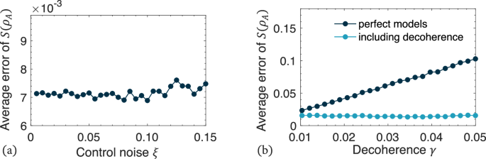
The prediction results for the subsystem entropy (S({rho }_{A})=-log (,text{tr},{rho }_{A}^{2})) of the four-qubit test data are shown under control noise (a) and decoherence noise (b). Each control noise strength ξ and each decoherence strength γ is tested with M = 500 samples. The average error, defined as the average distance between the actual entropy and the predicted entropy, is calculated as (epsilon =frac{1}{3M}mathop{sum }nolimits_{m = 1}^{M}mathop{sum }nolimits_{{rho }_{A} = [1]}^{[123]}| {S}_{m}^{{rm{th}}}({rho }_{A})-{S}_{m}^{{rm{ML}}}({rho }_{A})|).
Then, we outline how to enhance the robustness of the machine learning method against decoherence. A natural approach is to incorporate the decoherence effect into the training models. In this scenario, we create the training data using the following steps: First, we compute the ground states ({rho }_{g}=vert {psi }_{g}rangle langle {psi }_{g}vert) of random Hamiltonians and then obtain the decoherence state ρd using Eq. (5). Next, we calculate single- and two-qubit correlated Pauli expectation values as input data and the subsystem entropy as output data. After training the machine learning model, we use it to predict the entropy of the test data. Figure 7c displays the test results, showing improved robustness against the decoherence effect compared to models trained on perfect Hamiltonians. In a summary, our machine learning method has a good robustness against the control noise in the quantum circuit preparing the states. To improve the practicality of our method in the more noise resources, we can use noisy training data to train the neural networks models instead of perfect Hamiltonian models.
The guard against adversarial situations
Practically, there may be some adversarial situations in which unscrupulous actors produce unentangled (or nearly unentangled) states to deceive us. Here, we test the performance of our machine learning method in two adversarial situations. First, suppose there is an unscrupulous actor who generates separable states (leftvert {psi }_{AB}rightrangle =leftvert {psi }_{A}rightrangle otimes leftvert {psi }_{B}rightrangle) in an attempt to deceive us. These states, (leftvert {psi }_{AB}rightrangle), are the ground states of separable Hamiltonians ({mathcal{H}}={{mathcal{H}}}_{A}otimes {{mathcal{H}}}_{B}), where ({{mathcal{H}}}_{A}) and ({{mathcal{H}}}_{B}) are random Hamiltonians with internal interactions but no interaction between them. In this scenario, there is no entanglement between parts A and B. To verify if our method accurately identifies entanglement between A and B, we randomly generate some states (leftvert {psi }_{AB}rightrangle) with A = [12] and B = [34] and use our machine learning method to measure the second-order Rényi entropy (S({rho }_{A})=-log (,text{tr},{rho }_{A}^{2})). Figure 8 shows our method’s prediction SML(ρA) for 500 test samples of (leftvert {psi }_{AB}rightrangle). The results demonstrate that SML(ρA) is close to the true value Sth(ρA) = 0 for A = [12]. Therefore, our method does not significantly overestimate the entanglement between A and B. Second, we image a scenario where an unscrupulous actor creates fully separable states (leftvert Psi rightrangle ={otimes }_{i = 1}^{N}leftvert {psi }_{i}({theta }_{i},{phi }_{i})rightrangle) to deceive us. The state (leftvert {psi }_{i}({theta }_{i},{phi }_{i})rightrangle ={R}_{z}({theta }_{i}){R}_{y}({phi }_{i}){leftvert 0rightrangle }^{otimes N}) is a random state on the Bloch sphere. (leftvert Psi rightrangle) is an unentangled state with zero entropy across all subsystems. We then apply our machine learning method to determine the entropy SML(ρA) for A = [1], [12], [123] in 500 four-qubit states (leftvert Psi rightrangle). The test results, presented in Fig. 8b, show that the predicted entropies SML(ρA) closely match the true value of Sth(ρA) = 0. Therefore, we can establish an entanglement threshold to guard against unscrupulous actors. If the predicted entanglement by the machine learning model falls below a threshold, say 5 × 10⁻³, we consider the state to be either unentangled or nearly unentangled. Of course, our method is primarily designed to detect entanglement in states prepared in our own trusted and controlled laboratory (nonadversarial situations). While detecting entanglement in adversarial situations is a valuable research direction for the future, it is beyond the scope of our current work.
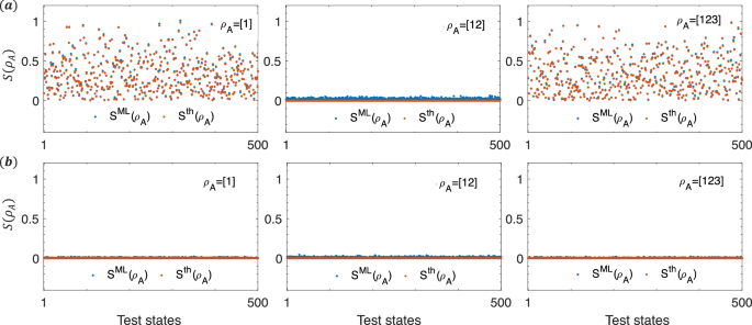
a The predicted entropies of the separable Hamiltonians ground states. b The predicted entropies of the fully separable states. For each adversarial situation, we tested M = 500 samples. The red points represent the actual entropy of the subsystem, while the blue points indicate the predictions made by our machine learning method.
The predictions for oscillating rapidly entanglement dynamics
Our idea of predicting entanglement behavior after the training period was inspired by our previous work, which aimed to learn Hamiltonians from single-qubit time traces alone, without quantum process tomography46. If single-qubit time traces during the training period suffice to determine the Hamiltonian model, the dynamics governed by this model should also be predictable, even after the training period. It inspired us to predict entanglement behavior using only single-qubit time traces from the training period. Our numerical and experimental results confirm that this idea is feasible in some contexts. In the previous text, we chose specific Hamiltonian parameters (J = −0.5, g = −0.3) and (J = −0.5, g = −0.75) to exhibit dynamical quantum phase transitions for the model ({{mathcal{H}}}_{d}=Jmathop{sum }nolimits_{i = 1}^{4}{sigma }_{z}^{i}{sigma }_{z}^{i+1}+gmathop{sum }nolimits_{i = 1}^{4}{sigma }_{x}^{i}), such that changes in entanglement primarily occur during the training period. To further validate the feasibility of our method in extreme situations, we have also tested 100 Hamiltonian ({{mathcal{H}}}_{d}) with random J and g, as shown in Fig. 9a, b. Figure 9c presents some results of extreme test samples, whose entanglement dynamics oscillate rapidly over the unmeasured time window [π, 2π], even after the training period [0, π]. It is important to emphasize that our work requires time-independent Hamiltonians. If the Hamiltonian models are time-dependent, predicting entanglement dynamics after the training period becomes essentially impossible because the Hamiltonians after the training period are different from that in the training period.
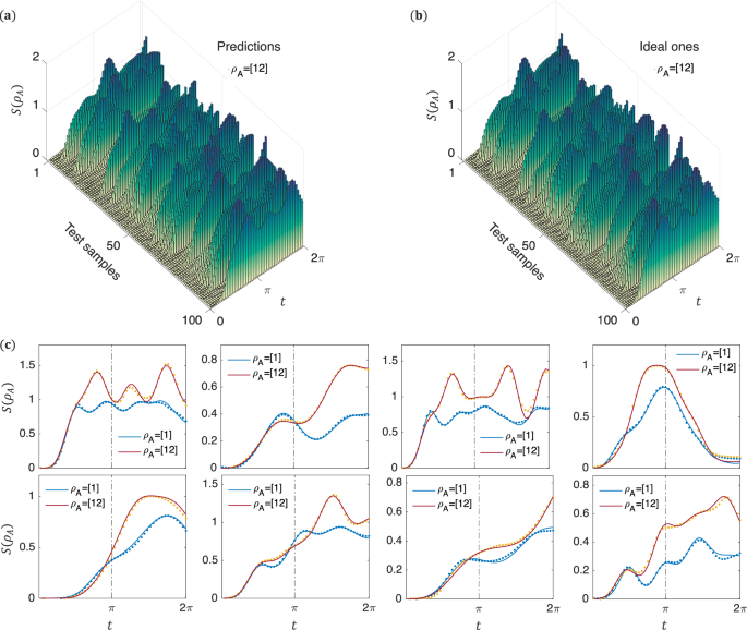
a, b We present a comparison between the machine learning predictions SML(ρA) and the theoretical values Sth(ρA) for subsystem ρA = [12]. c Showcases test samples that exhibit rapidly oscillating entanglement dynamics following the training period [0, π]. The lines represent the theoretical values, while the points indicate predictions made by the machine learning model. This model uses only the single-qubit time traces from the training period [0, π] as inputs and predicts the entanglement dynamics throughout the entire time window [0, 2π].
The scaling of training points as qubits
The number of training points is a crucial parameter for our machine learning method. In this section, we both qualitatively and quantitatively analyze the required number of training points. The number of training points depends on the complexity of the Hamiltonian models. In our study, we consider N-qubit random two-local Hamiltonians with polynomial degrees of freedom in terms of magnetic field strength and coupling. Generally, a polynomial amount of training data, O(Nc), with a constant c, is usually required to train machine learning models. We also numerically trained and tested different machine learning models with varying numbers of training points and qubits. Here, we considered one-dimensional random Hamiltonians ({mathcal{H}}) described in Eq. (1), which contain 12N − 9 free parameters. The performance of the trained neural networks was measured using the average error (epsilon =frac{1}{M(N-1)}mathop{sum }nolimits_{m = 1}^{M}mathop{sum }nolimits_{{rho }_{A} = [1]}^{[123..]}| {S}_{m}^{{rm{th}}}({rho }_{A})-{S}_{m}^{{rm{ML}}}({rho }_{A})|), which represents the average distance between the theoretical entanglement ({S}_{m}^{{rm{th}}}) and the prediction results ({S}_{m}^{{rm{ML}}}) of the neural networks. M denotes the number of test data points. Figure 10a shows the average error ϵ as a function of the number of qubits and the number of training points. The results indicate that 100,000 training points are sufficient for most examples in our work, and even fewer points, like 60,000, can be used for 6-qubit. The blue line with ϵ ~0.01 demonstrates that the number of training points scales favorably with system size.
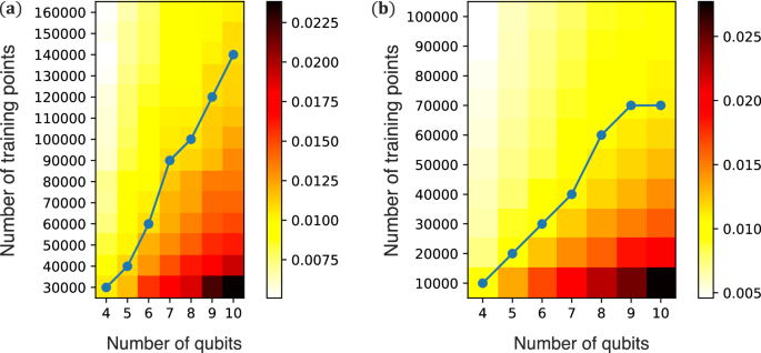
a Test results for Hamiltonian ({mathcal{H}}) described in Eq. (1). b Test results for Hamiltonian ({{mathcal{H}}}_{{rm{XY; Z}}}). The blue line is plotted where ϵ is around 0.01. ϵ is defined as (frac{1}{M(N-1)}mathop{sum }nolimits_{m = 1}^{M}mathop{sum }nolimits_{{rho }_{A} = [1]}^{[123]..}| {S}_{m}^{{rm{th}}}({rho }_{A})-{S}_{m}^{{rm{ML}}}({rho }_{A})|).
If the number of free parameters in the Hamiltonian model is limited, even independent of system size, the number of training points will scale more favorably with the problem size. For instance, a recently related work used only 300 training points to train the 64 × 64 lattice model because its Hamiltonian model had only two free parameters47. We also trained and tested a simpler Hamiltonian model, the XYZ spin chain Hamiltonian
which has 6N − 3 free parameters. Figure 10b shows the average error ϵ as a function of the number of qubits and the number of training points. Only 70,000 training points were sufficient to make ϵ around 0.01 for 10-qubit.
Our machine learning models are trained using classical simulations. Concerns may arise regarding the feasibility of experimental training and the scalability of classical training. First, it is well-known that the purpose of using machine learning techniques is to address challenging problems in quantum physics. Supervised machine learning generally involves training neural networks on training data with well-defined labels (such as entanglement detection, as in our study). If we require neural networks to be trained in experiments, then the labels must be easily measurable and identifiable in experiments, which contradicts the intent of using machine learning to predict physical quantities that are difficult to measure experimentally. For example, there are some studies also conducted training via classical simulations before directly predicting labels that are hard to measure in experiments48,49,50. Second, it remains feasible to simulate larger systems with over a hundred qubits using tensor network techniques. Currently, most quantum processors, including superconducting circuits, ion traps, quantum dots, and cold atoms, can control dozens to hundreds of qubits. At this scale, classical computers can still simulate their quantum circuits and dynamics with the help of tensor network techniques, but it is nearly impossible to measure entanglement through quantum state tomography for more than ten qubits. Previous experiments indicate that ten-qubit quantum state tomography takes about five days, while 20-qubit tomography would take ninety years51.
To demonstrate the feasibility of training models with more qubits, we trained machine learning models for Hamiltonians with 100 qubits, using various training data sizes, which were simulated and generated using tensor network techniques. Figure 11 shows the corresponding test results, indicating that 400,000 training points suffice to train a machine learning model for 100-qubit Hamiltonian ({{mathcal{H}}}_{{rm{XY; Z}}}). Hence, our machine learning method provides a promising approach for measuring entanglement in systems with dozens to hundreds of qubits. This approach represents the fundamental motivation behind using supervised machine learning to tackle challenging problems in quantum physics today.
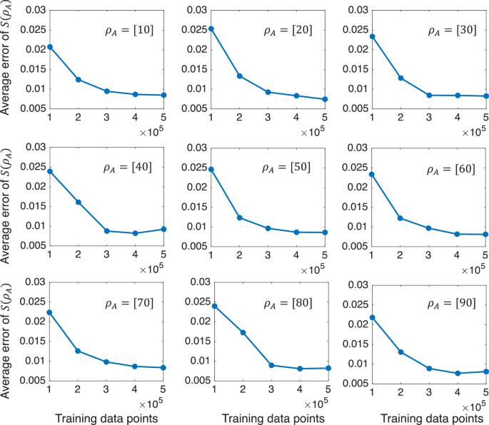
ϵ is defined as (epsilon =frac{1}{M}mathop{sum }nolimits_{m = 1}^{M}| {S}_{m}^{{rm{th}}}({rho }_{A})-{S}_{m}^{{rm{ML}}}({rho }_{A})|). ρA = [n] denote the subsystems of the first n qubits of 100-qubit.
In summary, we have developed a machine learning-assisted strategy to infer entanglement information from local measurements across both ground and dynamical states, effectively bypassing the need for quantum full-state tomography (FST), which typically requires an exponential number of measurements. Our method demonstrates robustness against control noise in quantum circuits used for state preparation. In addition, by incorporating noise into the training data rather than relying on ideal Hamiltonian models, we enhance the robustness against decoherence. The models are also equipped to guard against potential manipulation by unscrupulous actors who might introduce unentangled (or nearly unentangled) states to deceive the system. The number of training points varies with the complexity of the Hamiltonian models; for Hamiltonians with polynomial degrees of freedom, the scaling of training points with system size is favorable. Moreover, for dynamical states, our neural networks are capable of monitoring long-term entanglement dynamics, even those that oscillate rapidly, for future times unseen. We have further validated the practicality of our approach in 4-qubit NMR experiments. These results enhance the feasibility and reliability of our machine learning method in real-world applications, offering a promising method for experimentally measuring entanglement in systems ranging from dozens to hundreds of qubits.
Our approach directly measures the expectation value of the local Pauli operator, which is very easy to implement experimentally, while typical work that directly predicts entanglement via machine learning requires measurements of partially transposed moments as input, which is very difficult to implement23. Classical shadows and the randomized measurement toolbox are two well-known methods for estimating entropy that work for arbitrary states22,24, and they achieve more accurate entropy estimation with sufficient measurements, as they can manage a broader range of errors, but they require exponential measurements in the subsystem size. Our approach is applicable to structured quantum states, such as ground states and dynamical states of quantum many-body Hamiltonians, but requires only polynomial measurements. In this way, they constitute complementary relations and are suitable for different applications in measuring entropy. Our numerical experiments on the ground state clearly show that our method requires fewer measurements than them, and the discrepancy increases as we require larger sizes (see the Supplemental Material for details).
Our neural network strategy has the following extensions and future applications. The previous research has demonstrated that some quantum states can be determined using compressing sensing52,53, direct estimation54, and the UD-property (Uniquely Determined, UD)17. These techniques normally measure random or fixed Pauli measurements. This means that by creating a nonlinear map with quantities like local expectation and entanglement, we can extend our framework to various types of quantum states, such as UD-property quantum states55. Second, our framework will have wide applications in studying the intriguing equilibrium and non-equilibrium phenomena56, because the entanglement entropy is an essential quantify that diagnoses and characterizes QPTs57, quantum thermalization26, and quantum MBL58.
Methods
The construction of neural networks
In this section, we provide a detailed description of the neural network model training and testing scheme. Neural networks are based on a collection of connected units, or nodes, called artificial neurons, that can learn the input-output mapping relation of a data set. For a single neuron, the received input signals are combined linearly, and then the combined signals are further processed by a nonlinear operator (activation function) which can improve the nonlinear learning ability of the neural network. There are various state-of-the-art neural network models devised by combing neurons with different techniques, e.g., fully connected neural networks, convolutional neural networks, residual neural networks, recurrent neural networks, and attention mechanisms.
We will focus on the following three tasks. The first is to predict the static entanglement quantities ({mathcal{E}}) from the measure data ({mathcal{O}}) on ground states, the second is to predict the corresponding entanglement information ({mathcal{E}}(t)) from the measured data ({mathcal{O}}(t)) on dynamical states, and the third is to extrapolate the entanglement entropy at subsequent moments from the data in the previous moments. Thus, we need to prepare two different types of training/testing sets. The first kind of data set is static data, and the index of the input tensor is X = [M, Din], where M is the number of data in the data set, and Din is the dimension of the input. Similarly, the output tensor is Y = [M, Dout], where Dout is the dimension of the output. The second type of data set is dynamic data, the input tensor is X = [M, Din, T], where T is the number of time steps, and the output tensor is Y = [M, Dout, T].
Fully connected neural networks, also known as multilayer perceptrons, are multilayer neuronal architectures composed mainly of input, hidden, and output layers. Mathematically, the calculation of the l layer with nl neurons, g( ⋅ ), can be expressed as follows:
where ({{bf{x}}}^{(l)}in {{mathbb{R}}}^{{n}_{l}}) is the output of the l-th layer and also is the input of the l + 1 layer, ({{bf{x}}}^{(l-1)}in {{mathbb{R}}}^{{n}_{l-1}}) is the input of the l-th layer, ({{bf{A}}}^{(l)}in {{mathbb{R}}}^{{n}_{l}times {n}_{l-1}}) is the weight matrix which is consisted of nl ⋅ nl−1 training parameters θ, ({{bf{b}}}^{(l)}in {{mathbb{R}}}^{{n}_{l}}) is the bias which consists of nl training parameters θ and f(⋅) refers to the activation function. Thus, an FCNN with L layers can be given as:
where yout is the output of FCNN, xin is the feature of data.
Long Short-Term Memory (LSTM) is a form of recurrent neural network (RNN) with internal states (memory) to learn the serial correlation of data. It has been widely used for time series forecasting and has been shown to perform well for both long-term and short-term forecasting. While fully connected networks are state-of-the-art in many problem scenarios, they do not handle complex time series problems well. Unlike FCNN, which cannot receive the outputs of previous time steps and use them as inputs for the current time step, LSTM networks can encode information from previous moments in the internal state. An LSTM consists of a chain of repeated neural network blocks called LSTM Cells. Therefore, LSTM has been widely used in various time series analysis tasks in the quantum domain, such as natural language processing, quantum control, and quantum process tomography. For the tth time step LSTM computation, it can be expressed as follows:
where ht is the output of the tth LSTM cell which is also called the short-term state, ct is the cell state of the tth LSTM cell, and xt is the input at time t and F (⋅) is the essential part of the LSTM called LSTM cell. The LSTM cell consists of a long-term memory structure called cell state c which encodes the information in neural network, and three control gates, forget gate f(⋅), input gate i(⋅) and output gate o(⋅), to control cell state updates and output. Denote that × as a point-wise dot, + as a point-wise add, σ as the sigmoid activation function and tanh as the tanh activation function. Mathematically, we can formulate the three control gates as follows.
-
(1)
the forget gate is given as
$$f({h}_{t-1},{{bf{x}}}_{t})=sigma left({Theta }_{g}cdot left[{{bf{h}}}_{t-1},{{bf{x}}}_{t}right]+{b}_{g}right)$$
which determines how much information about the current inputs xt and the memory information ht−1 provided in the previous step should remain. Here and in the following, the tensors Θ and b are the weight and bias parameters of the LSTM cell, respectively. We label their corresponding gates with different subscripts.
-
(2)
the input gate is given as
$$i({{bf{h}}}_{t-1},{{bf{x}}}_{t})=sigma ({Theta }_{i}cdot [{{bf{h}}}_{t-1},{{bf{x}}}_{t}]+{b}_{i})$$
which indicates how much input information should be received in the current LSTM cell.
-
(3)
the output gate is given as
$$o({{bf{h}}}_{t-1},{{bf{x}}}_{t})=sigma left({Theta }_{o}cdot left[{{bf{h}}}_{t-1},{{bf{x}}}_{t}right]+{b}_{o}right).$$
This determines which information should be kept and passed to the output. With the above three control gates, the entire LSTM cellular information processing flow can be written as follows. First, the current input xt and the memory information ht−1 provided in the previous step are encoded into the candidate cell state (widetilde{{{bf{c}}}_{t}}) by the tanh activation function.
Then, candidate cells are then complemented with forgetting and input gates to update them to a new cell state. ct.
Finally, short-term state ht is output by combining output gate and cell state
Thus, LSTM output is (widetilde{{{bf{y}}}_{t}}) as follows:
In order to predict the corresponding entanglement entropy through the input time series data and extrapolate the entanglement entropy at the subsequent time. Since the error in the extrapolated part is larger than the error in the first half, the error gap between the two parts is too large. It is difficult to use the mean squared error as a loss function to train a network model for entanglement entropy estimation and extrapolation. The task is split into two, the first is to extrapolate the second half of the observations from the first half, and the second is to estimate the entanglement entropy by feeding in all observations. Thus, we need to train two LSTM-based encoder-decoder network models separately. The first network needs to output the estimated last half of the observations by inputting the first half of the timestep, which is called the extrapolation network. The second network, where the input is all observations and the output is the estimated entanglement entropy, is called the estimation network.
Training neural networks
Mean square error (MSE) is widely used to evaluate the accuracy of the models. The MSE represents the difference between the predicted value and the actual value.
By calculating the MSE between the estimated result of the neural network and the entanglement entropy of the training sample data, and using this as the loss function, the gradient algorithm is used to optimize the weighted network parameters, so as to learn the mapping relationship between the observation and the entanglement entropy.
The most common way to train a neural network is a supervised learning algorithm based on the gradient descent algorithm, such as stochastic gradient descent (SGD), momentum SGD, root mean square prop (rmsprop), adaptive moment estimation (ADAM), etc. Due to the nested layer-by-layer nature of deep networks, when computing the gradient of an objective function of a deep network, the parameters can be updated more quickly by using backpropagation to compute and update the parameters backward from deep to shallow layers. To explain how the neural network is optimized, we assume that the SGD algorithm is the optimizer, and then for a neural network, the weight parameter is Θ, and the loss function is L. So the kth optimization iteration can be written as
where M is the size of the batch, and α is the learning rate. Moreover, in order to smooth the training and improve the robustness of the model, it is necessary to perform weight decay on the loss function, also known as L2 regularization, which is a regularization technique applied to the weights of a neural network. By weight decay, we write the final loss function as follows.
where λ is a value determining the strength of the penalty. In this paper, ADAM is the best algorithm for training a neural network. Compared to the SGD algorithm, it converges faster and adaptively adjusts the learning rate. After training, the neural network model is saved and the test set is used to test the accuracy of the estimated entanglement entropy and the robustness of the neural network.
Experimental setup
In order to implement entanglement measures using our neural networks in real physical systems, we conduct a series of experiments. All experiments were implemented on a Bruker AVANCE 600 MHz spectrometer at room temperature (298 K). We chose 13C-labeled crotonic acid as the four-qubit quantum processor, consisting of four isotope carbon atoms as spin qubits. The internal Hamiltonian of this sample is,
where ωi is the chemical shift and J is the J-coupling strength. Among the molecule, the four 13C atoms C1, C2, C3, and C4 are corresponded to four qubits of the 4-qubit quantum processor. The structure and parameters of the molecule are shown in Fig. 12. Single-qubit quantum gates are implemented using radio-frequency (RF) pulses of specified shapes, while two-qubit quantum gates are realized through the coupling between qubits. To prepare the ground states and dynamical states used in our experiments, we optimize shaped pulses using gradient ascent pulse engineering. By detecting the free induction decay signal of the final states, we can extract the expectation values of single-qubit and two-qubit Pauli operators, which are used as inputs for our neural networks.
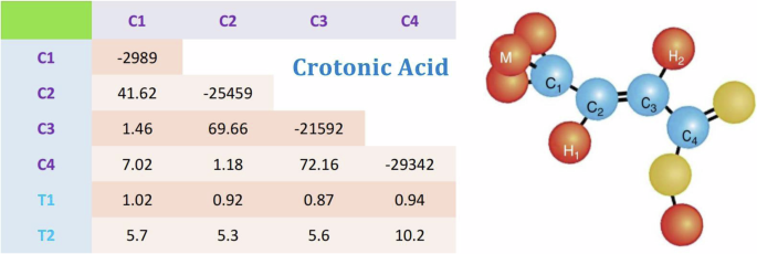
In experiments, C1, C2, C3 and C4 form a 4-qubit quantum processor. In this table, the chemical shifts with respect to the Larmor frequency 150 MHz and J-couplings (in Hz) are given as the diagonal and off-diagonal elements, respectively. The methyl group M, H1 and H2 were decoupled throughout all experiments.
Responses