Discovering dominant dynamics for nonlinear continuum robot control

Introduction
In an era where the convergence of robotics and the natural world is set to redefine the boundaries of exploration, interaction, and intervention, our endeavor to engineer robots capable of navigating and manipulating their environment with the grace of living organisms has never been more pertinent. At the forefront of this challenge is the field of continuum robotics, which, by emulating the fluid movements of biological systems, presents unprecedented opportunities for innovation across a broad range of applications-from the unexplored depths of our oceans to the boundless expanses of space.
Unlike their rigid counterparts, continuum robots are characterized by their ability to assume an infinite range of shapes and movements within the bounds of their design. This unique characteristic affords them numerous advantages over their rigid counterparts, namely dexterous manipulation and locomotion, flexibility, and physical compliance. These advantages are ideal in various applications spanning multiple disciplines, as shown in Fig. 1. For example, soft surgical robots provide unparalleled precision and safety in navigating the complex and constrained environments of the human body1. In deep-sea exploration, soft robotic fish exhibit pressure resilience allowing scientists to push the boundaries of scientific discovery and explore the deepest parts of our oceans2. Space satellites equipped with deformable manipulators will allow for more precise space debris removal and satellite servicing operations3,4, while continuum robots will enable us to explore internal and enclosed dynamic terrain structures of scientific interest on Mars and Enceladus5. In all these applications, the robots must operate safely with precision under computational constraints.

a Phase portrait and 1-dimensional invariant manifold of a damped pendulum. b Origami-inspired artificial muscles as a deployable structure for on-orbit rendezvous operations. (PNAS60). c Electrically-driven bionic trunk made out of shape memory alloy with potential application to minimally invasive surgery (Wiley61). d A pressure-resilient, soft robot fish that can operate in deep sea trenches. e Illustration of the eigenvalues of the linear part of the high-dimensional system, with the dominant modes being the eigenvalues closest to the imaginary axis. The SSM is parameterized by these slow modes and carries the dominant dynamics of the system.
The distinctive characteristics that grant continuum robots their flexibility and dexterity also present significant challenges in their modeling and control. Their compliance and intricate motion capabilities lead to complex dynamics, driven by both geometric and material nonlinearities6,7 as well as nonlinear resonances. Accurately capturing these dynamics typically requires high-dimensional, nonlinear models which in turn poses computational challenges for real-time control. Moreover, the inherent deformability of these robots complicates the design of effective sensing systems to detect and measure their dynamic behavior8. Despite these challenges, there is hope to tractably model these systems for control. Continuum robots are highly dissipative, thus despite their high dimensionality, their high-frequency degrees of freedom rapidly synchronize with the robots’ low-dimensional, persisting dynamics, i.edominant dynamics. Additionally, by carefully choosing the robot’s sensor modality and arrangement, one can uncover these dominant dynamics from observed measurement transitions. The emergence of machine learning (ML) carries the promise of unveiling these dynamics from data at great fidelity.
This work addresses the task of achieving precise and safe control of continuum robots under computational constraints. To this end, we seek the following desiderata to learning dynamics for model-based control:
-
1.
Faithful models: The algorithm should learn highly predictive models that generalize across different operating regimes, enabling precise control across a variety of tasks.
-
2.
Low model complexity: The model should be sufficiently low-dimensional to enable real-time control in resource and compute-constrained hardware.
-
3.
Data efficiency: The learning algorithm should require a small, yet sufficient sample size to extract a performant model, making it feasible to train models with limited real-world data.
-
4.
Sensor efficiency: To facilitate observability, the learning methodology should be able to incorporate data from as many sensors as available on the robot without increasing the model’s complexity.
-
5.
Safety constraints: The control scheme should be able to handle state and actuation constraints, allowing the system to operate in safety-critical settings.
Existing methodologies have yet to satisfy these desiderata, largely due to their inability to discern the dominant dynamics governing continuum robot behavior in a mathematically precise fashion. These methodologies typically divide into two camps: those that learn a direct control policy and those that create a surrogate model for control.
Model-free reinforcement learning (RL) is an approach where the robot learns to make decisions by taking actions in its environment to maximize some notion of cumulative reward. Since continuum robots have intricate dynamics and are high-dimensional in nature, these approaches have gained traction in the literature9 as they bypass the necessity to explicitly model these complexities. Model-free RL has proven effective across various robot designs and control tasks, ranging from real-time control of dynamic maneuvers10 to locomotion in soft robotic fish11. Despite these successes, model-free RL lacks inherent safety guarantees during the exploration phase in which agents may take unsafe actions while learning. While some methods have been developed to address these safety concerns12, they often increase the computational complexity and require more conservative exploration strategies, which may limit generalizability and data-efficiency. This limits the practicality of applying RL to continuum robots operating in safety-critical environments.
As a result, much of the continuum robot literature leverages data-driven methods to infer the dynamic models of continuum robots for control. One strategy involves using data to find an optimal compression of the robot’s finite-element model to a lower-dimensional representation13,14,15. However, this often results in reduced models that remain too large for real-time MPC on embedded systems with longer prediction horizons and higher control frequencies. This can make controllers less robust to model mismatch and overly focused on short-term actions, leading the system into states where it cannot effectively handle constraints. Furthermore, the development of high-fidelity analytical governing equations for compression is a cumbersome and ad-hoc process. As an alternative to this hybrid approach, learning the dynamics from time-series data of observed measurements using neural networks (NN) has become popular16,17,18,19. Despite their success in closed-loop control, these methods share the data inefficiency and generalization challenges seen in RL20. Another promising avenue in data-driven control involves systems-theoretic approaches. These leverage the Fundamental Lemma from behavioral systems theory to predict input-output trajectories directly from data while offering rigorous guarantees on stability, robustness, and constraint satisfaction21,22. Such approaches, however, typically require sufficiently rich data encoded in large data matrices to ensure accurate predictions, which can render them computationally intractable for real-time control23. Moreover, their effectiveness has yet to be demonstrated on the complex, high-dimensional dynamics of continuum robots.
Alternatively, data-driven modeling approaches grounded in Koopman operator theory24 have been demonstrated to achieve notable performance on various soft robot applications25,26,27. Approaches like Dynamic Mode Decomposition (DMD)28 and Extended DMD (EDMD)29 can be interpreted as approximations to an infinite-dimensional operator that linearly represents the system dynamics through observable functions in a function space. These methods yield linear models conducive to fast and efficient control design and boast greater data efficiency than NNs25. However, a major pitfall with these linear procedures is their reliance on finite-dimensional approximations to an inherently infinite-dimensional operator. For these methods to generalize, the chosen observables must span a finite-dimensional Koopman-invariant subspace, which occurs with probability zero, even for generic observables30. While one might hope to overcome this limitation by enlarging the dimension of observables, such enlargements often require hundreds or thousands of dimensions. This can lead to overfitting, where the model fits training data well but struggles to generalize to unseen trajectories31,32,33,34. Furthermore, the dimensionality of these linear models scales exponentially with the number of observables and basis functions. These limitations are fundamentally at odds: increasing the expressivity of the model to better capture the nonlinear dynamics leads to an exponential increase in model dimension. Not only does this restrict robot design and sensing capabilities, it also fundamentally limits the model’s accuracy because onboard compute constraints prevent the deployment of such large models.
To overcome these challenges, we leverage Spectral Submanifold Reduction (SSMR)35, an emerging modeling paradigm that was developed less than a decade ago and only recently introduced to the field of ML36,37. Originally conceived to model non-linearizable phenomena in engineering applications38,39,40, SSMR’s application to control was recently established41,42,43,44 due to two key model features: high predictive capability and low dimensionality. Spectral Submanifolds (SSMs) are attracting invariant manifolds residing in the robots’ phase space and learning the internal dynamics of these structures leads to faithful, low-dimensional models because all nearby trajectories converge to these dynamics exponentially fast. Consequently, the low-dimensional dynamics on SSMs are the de facto dominant dynamics that can efficiently be leveraged for real-time control of the robot. SSMs have also been shown to vary smoothly with respect to general control forces45, which makes the inclusion of control in the SSM-reduced dynamics possible.
In this work, we present a model-based control methodology based on SSMR which satisfy the aforementioned desiderata and advance earlier results42,43 towards,
-
(a)
making the procedure for learning dominant dynamics with arbitrary observables more rigorous and practical,
-
(b)
evaluating our proposed models on different robot morphologies in both high-fidelity simulation and hardware platforms,
-
(c)
aggregating these results to provide a novel methodology to address control of continuum robots.
Our method consistently improves the state-of-the-art along multiple dimensions including model accuracy by up to a factor of 6 and tracking performance by up to a factor of 150. Furthermore, our methods exhibit Pareto dominance with respect to baseline methods along both accuracy and computational efficiency. These previously unattainable results highlight the importance of inferring dominant dynamics for effective model-based control. Critically, in contrast to other data-driven methods which fit to individual trajectories, SSMR discovers robust (i.e structurally stable) phase space structures, and uncovers their internal dynamics with high accuracy. This advancement brings us closer to deploying highly adaptive, efficient, and safe continuum robots across various application domains.
Results
In this section, we present our approach to modeling and controlling nonlinear, continuum robots with limited training data and computational resources. We first address the practical challenges of limited sensor measurements and propose a solution that allows us to leverage the dominant dynamics for control. We then conduct a thorough comparison with current state-of-the-art methods, including a robustness study to assess the generalization capability of each model to trajectories well outside the training distribution. Our evaluation focuses on the predictive accuracy over a finite horizon as well as closed-loop performance, both with and without constraints. We conduct a Pareto analysis to assess the tradeoff between tracking error and solve time, evaluating the real-time feasiblity of each model.
Our baselines include the trajectory piecewise linearization (TPWL) model reduction approach13, DMD46, Koopman (often referring to EDMD)26, and the recent Koopman static pregain method25. We learned DMD and Koopman models using a modified version of26 and TPWL models using13. Since the performance of DMD and Koopman is sensitive to the user-specified regularization and model dimension, we learned multiple models corresponding to different parameters. We then chose models that achieved the best tracking performance on slow, i.e quasi-static control tasks, while still being computationally tractable. In TPWL, the model dimension is determined by the subspace to which we project the high-dimensional finite-element model. We find the optimal dimension by conducting singular value decomposition (SVD) on training trajectories and retaining the singular values which explain over 99.99% of variance in the dataset. The models deployed in simulation and hardware are outlined in Table 1.
We validate our findings through high-fidelity finite-element simulations on a diamond-shaped soft robot with 9768 dimensions and an elephant-inspired trunk robot with 4254 dimensions47. These differing robot morphologies are shown in Fig. 2a. Additionally, we conduct real-world experiments on a physical realization of the diamond robot for both unconstrained and constrained control tasks. The simulated and experimental diamond robots are made of soft silicone and actuated by motors which pull on cables attached to the robot’s four elbows. The addition of cable tension controls the robot’s deformation, allowing it to move continuously within its workspace. The trunk robot is also made of soft silicone but is controlled by eight cables, four of which terminate at the midpoint of its structure with the other four terminating at the endpoint. The robot is actuated by motors which pull on the cables, allowing it to assume a variety of geometries to navigate its workspace.
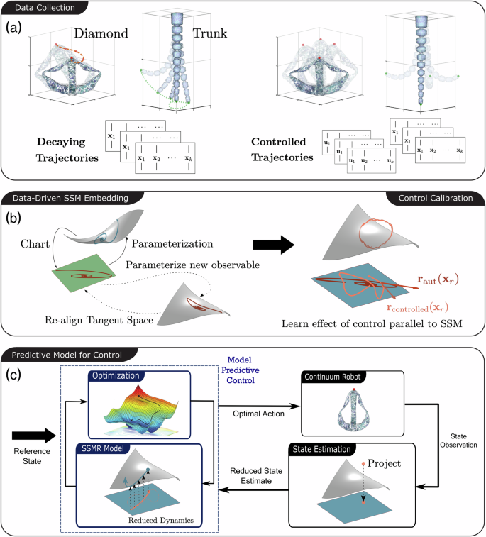
a Collect decaying and controlled trajectories of the continuum robot. The decaying trajectories are truncated to remove initial transients, ensuring the data is close to the slow, attracting SSM of preselected dimension. Critically, the decaying trajectories will characterize the structure of the autonomous SSM while controlled trajectories will calibrate the internal dynamics of this invariant manifold as it smoothly deforms under control. b Use SSMLearn36 to extract the dominant dynamics of the continuum robot on the autonomous SSM. Optionally, we can reparameterize the SSM to obtain a model with observables more favorable for control. Lastly, the calibration step learns the effect of control parallel to the autonomous manifold. c The SSMR-based, control-oriented model is used in a model predictive control scheme where planning and control is conducted in the reduced coordinates that parameterize the SSM.
Spectral Submanifold reduction for optimal control
To achieve precise, real-time control of nonlinear continuum robots, we uncover their inherently low-dimensional dynamics on SSMs. These SSMs are invariant manifolds that carry the robots’ dominant dynamics. Intuitively, there are two types of SSMs: autonomous SSMs, fixed at an equilibrium of the uncontrolled system, and non-autonomous SSMs, which evolve over time with the controlled system. Based on rigorous mathematical results from45, we approximate the dominant dynamics associated with the true, non-autonomous SSM by training on generic measurement data taken near an autonomous SSM. While in practice our data will almost never lie exactly on the primary SSM, it will lie with probability one on a nearby invariant manifold (i.e secondary SSM), of which infinitely many exist and whose Taylor expansion has the same leading order terms48. Subsequently, we identify the impact of control on the SSM-reduced dynamics via calibration. This procedure is summarized in Fig. 2.
First, we collect data tailored to approximate the autonomous SSM, as shown in Fig. 2a. This approach requires two datasets: a collection of decaying trajectories from different initial conditions and a collection of controlled trajectories. The decaying trajectory data are collected through a series of training experiments, performed by randomly applying constant control inputs to the robot and then removing the control input to allow the robot to decay to its rest state. The controlled trajectory datasets are collected by applying a random sequence of smooth inputs to the robot in open-loop. The training process is sample efficient requiring similar or less amount of data to infer a performant model compared to data-efficient baselines, as shown in Table 1.
The observables we use to infer the dominant dynamics of the robot are time-delayed measurements of the x–y–z position of the tracking markers placed on the end-effectors of each robot. In this way, we target the slowest 6D SSM of the system to capture the slowest oscillatory dynamics in the 3D space. In general, the desired dimension of the SSM-based model equals the dimension of the slowest spectral subspace corresponding to the dominant modes of the linearized system. We infer this dimension via an SVD of the decaying trajectories dataset (i.e principal component analysis)36,49 by retaining the top six modes which capture more than 95% of the variance in the data. We stress that although this procedure is presented for a specific set of robots with measurements taken at their end-effectors, our approach applies to generic control systems42,45.
Second, to extract dominant dynamics on the SSM, we must uncover the SSM’s chart and parameterization map, along with its calibrated internal dynamics, as shown in Fig. 2b. The chart map (i.e encoder) is inferred via singular value decomposition on the training set of decaying trajectories. The parameterization map (i.e decoder) and internal dynamics are fit using a monomial basis and by minimizing reconstruction error and prediction, respectively. Models with nonlinear (i.e 2nd order terms or higher) maps and dynamics are referred to as SSMR models, while those with only linear terms are referred to as Spectral Subspace Reduction (SSSR) models. In the latter, rather than fit a manifold, we fit a linear subspace with linear internal dynamics. Overall, we obtain a low-dimensional dynamics model and an output map which relates the reduced coordinates to our desired observables.
Finally, we design a Model Predictive Control (MPC) scheme (as shown in Fig. 2c), which predicts the future states of the robot using our SSMR-based model to optimize control actions in real-time, while considering safety constraints. In summary, our MPC scheme plans in a drastically reduced space, then maps these predictions into our desired measurements on which we evaluate our cost function and state constraints. The receding horizon nature of MPC provides closed-loop feedback that robustly handles the uncertainties in our model. As the optimal control problem is non-convex, we approximate it as a series of convex problems50 making it tractable by using reliable convex optimization solvers. Given that the control scheme exploits the low-dimensionality of our model, we benefit from low computational overhead, which in turn enables real-time, safe control.
Practical challenges with time delays
Numerous factors, including cost, power, and geometric constraints, may limit the number of sensors we can place on our system. Despite these limitations, time-delayed measurements allow us to uncover the dominant dynamics from observed data. This is because with enough delays, embedding theorems51,52 guarantee that we can detect the dominant dynamics from measured transitions.
As the dimension of the SSM increases, the increased time delay requirements imposed by these theorems result in filtering of non-autonomous, controlled behaviors. We refer to this filtering phenomenon due to increased time delays as the “curse of delays.”
Recall that SSMR projects the delayed observables onto the leading singular vectors resulting from the SVD of the decaying trajectory dataset. These leading modes can be interpreted as principal component trajectories (PCT)53 which represent the dominant patterns of decay and capture the most significant modes of change in the system’s dynamics over time. The challenge is that for an increased number of delays, the decaying PCTs are less capable of representing transient trajectories. This is because projection to the PCTs effectively acts like a bandpass filter with respect to the frequencies of the PCTs, with decreasing bandwidth as the delays increase.
To overcome these practical challenges, we can reparameterize the time-delayed model to other observables (e.g. using fewer time delays) as long as the dimension of the observables is at least the same as the SSM. Section 4.3 gives more details on how to conduct such a procedure. To evaluate this claim, we learn two SSM models: one purely parameterized by nd ∈ {4, 10, 15, 20} delays and the other which reparameterizes the original nd model to a single delay observable. We then pass the figure-eight trajectory of the simulated diamond robot through the chart and parameterization maps of the two models at nd to evaluate its reconstruction accuracy. Since this trajectory is sampled every 10 ms, the delays correspond to the past Td ∈ {40, 100, 150, 200} ms (simulation time) of end-effector measurements.
Figure 3 shows that models featuring many time delays have low reconstruction accuracy. As suggested, reparameterizing the model to a single time delay results in almost constant reconstruction accuracy, despite the base model being of higher nd delays. Interestingly, we observed that both models exhibit good reconstruction accuracy for uncontrolled, decaying trajectories. This suggests that increased delays act as a bandpass filter with decreased passband about the frequencies of the principal modes detected in the decaying trajectories. Thus, if the desired control trajectory has a frequency different from the principal modes, increasing the number of delays will filter out important transients that characterize this trajectory. Thus, we adopt this reparameterization trick to construct SSMR and SSSR models with a single time delay, thereby avoiding the curse of delays.
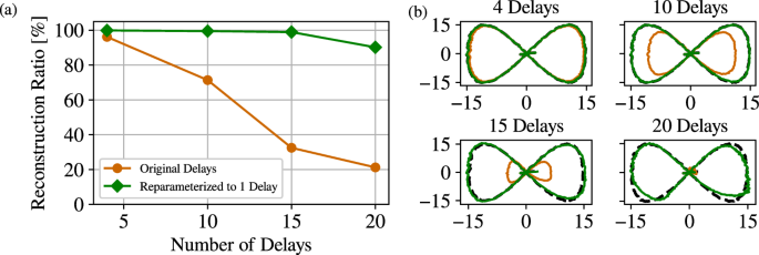
a Percent reconstruction of controlled trajectories of the diamond robot’s end-effector as a function of the number of delays in the model. The 0.744762,0.317516,0.028023orange plot shows the figure-eight’s reconstruction from a model with increasing time delays without reparameterization. The 0.054870,0.440281,0.010655green plot represents reconstruction for a model that is reparameterized to single time delay. b Qualitative depiction of the reconstruction of the figure-eight trajectory along the x–y plane for the original and reparameterized models.
Simulation open-loop prediction accuracy
In this section, we compare the predictive accuracy of our SSMR model against SSSR and established baselines in the literature. To conduct this evaluation, we explore the actuation space of the robot using a randomly sampled input sequence different from the ones used to learn both the SSMR and baseline models. We record the resulting open-loop trajectory and corresponding inputs, and at random, chose n = 500 points {p1, . . . , pn} along this trajectory. Starting from each point pi as an initial state, we roll out the system’s trajectory over the next five time steps using the respective segment of the original input sequence. We quantify predictive accuracy by calculating the Root Mean Square Error (RMSE) between the predicted and actual trajectories for each pi over a 50 ms horizon. By replicating this finite-horizon prediction process across all selected points, we achieve a comprehensive evaluation of our model’s accuracy throughout the robot’s configuration space. To provide further context on the dynamics of the trajectories, the average speed of the reference trajectory for the diamond robot was 74.7 mm/s, while that of the trunk robot was 30.3 mm/s.
Figures 4,5 show the simulation open-loop evaluations for the diamond and trunk robot, respectively. SSMR models achieve excellent predictive performance for both robots. Intuitively, this means that we approximate the 6D autonomous SSM well and that trajectories of the full system indeed synchronize fast with our model, which approximates the internal dynamics of the SSM. This results if the control minimally excites the outer modes, or if the effect of outer modes are insignificant due to large timescale difference between the dominant and off-manifold dynamics. In both cases, the off-manifold transients only occur momentarily and the dominant dynamics capture most of the robot’s behavior. In general, the SSMR models’ prediction accuracy degrades as the end-effector moves further from the robot’s uncontrolled, resting point. This is because our model includes only a first-order correction to the uncontrolled dynamics. To improve accuracy at positions further from the origin, we would need to include higher-order corrections.
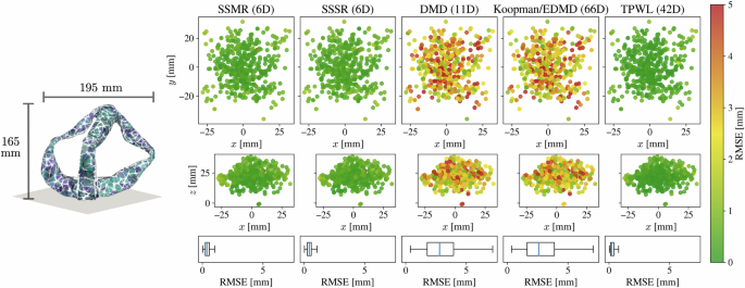
Open-loop performance of diamond robot models over a 50 ms horizon and evaluated across 500 different points along a given trajectory. The box spans the middle 50% of the data, with whiskers extending to the smallest and largest values within 1.5 times the interquartile range, and points outside the whiskers indicating outliers. The best performing model is TPWL with an RMSE of 0.317 mm. SSMR and SSSR give comparable performance at 0.492 mm and 0.457 mm, respectively. DMD and Koopman/EDMD give the worst average RMSE at 3.104 mm and 2.962 mm, respectively.
For the diamond robot, TPWL outperforms all other models in this evaluation but degrades in accuracy for the trunk robot. This indicates that the diamond robot’s behavior near this trajectory is close to linear. On the other hand, Koopman/EDMD and DMD exhibit the worst performance among all models. As expected, the Koopman/EDMD and DMD models in Figs. 4 and 5 exhibit no clear pattern in model accuracy with respect to the configuration of the robot. Since Koopman/EDMD and DMD will learn a Koopman-invariant subspace with probability zero, the Koopman/EDMD and DMD models overfit to their training data and do not generalize well to the evaluation dataset.
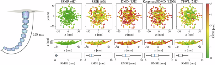
Open-loop performance of trunk robot models over a 50 ms horizon, evaluated across 500 different points along a given trajectory. The box spans the middle 50% of the data, with whiskers extending to the smallest and largest values within 1.5 times the interquartile range, and points outside the whiskers indicating outliers. The best performing model is SSMR with an average RMSE of 0.54 mm. TPWL comes next at 1.90 mm, while SSSR gives an average RMSE of 2.60 mm. DMD and Koopman/EDMD give the worst performance at 4.24 mm and 3.68 mm average RMSE, respectively.
Interestingly, SSMR only slightly outperforms the SSSR models on the diamond robot evaluations, indicating that the diamond robot’s behavior in this open-loop trajectory is nearly linear. This can be attributed to the robot’s truss-like structure, where most of the motion occurs at virtual hinges, leading to mostly linear behaviors. Furthermore, SSSR outperforms Koopman/EDMD and DMD on both robots, highlighting that our model discovery approach infers the underlying linear dynamics from data more accurately than fundamentally linear methods which attempt to approximate the Koopman operator. However, the SSSR model’s predictive accuracy deteriorates quickly further away from the robot’s resting position and, hence, performs worse overall than the SSMR models. This is clearly visible for the simulated trunk robot whose end-effector was made to follow trajectories further from its equilibrium position.
Simulated closed-loop trajectory-tracking performance
We now evaluate the closed-loop performance of the models on a variety of trajectory-tracking tasks. For these evaluations, the end-effectors of the robots were commanded to trace out various dynamic trajectories with a control frequency of 50 Hz and an MPC horizon of 100 ms. We evaluate trajectory tracking accuracy using the Integrated Squared Error (ISE) which sums the squares of the error over time. Like RMSE, it heavily penalizes larger errors, but it does so over the integral of the control process. For the diamond robot, we consider two 10 second long trajectories: a slow figure-eight trajectory at an average speed of 4.5 mm/s and a fast figure-eight at an average speed of 89.4 mm/s, both in the x–y plane. The results are shown in Fig. 6. For the trunk robot, we commanded its tip to follow two 10 second 2D trajectories in the x–y plane: one tracing the “ASL” symbol at an average speed of 11.9 mm/s, and the other tracing a Pacman symbol at 4.6 mm/s. The results for the trunk are shown in Fig. 7.
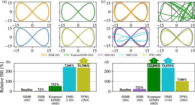
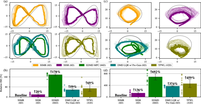
a Closed-loop trajectory for the slow figure-eight trajectory in the x–y plane with b Relative tracking ISE of SSMR for the slow figure-eight compared to the other models. SSMR and SSSR perform similarly while Koopman/EDMD performs noticeably worse. DMD and TPWL perform significantly worse than SSMR. c Closed-loop trajectory for the fast figure-eight trajectory in the x–y plane with d Relative tracking ISE of SSMR for the fast figure-eight. This desired trajectory is far from the training distribution and SSMR and SSSR are the only models that remain robust to this out-of-distribution task.
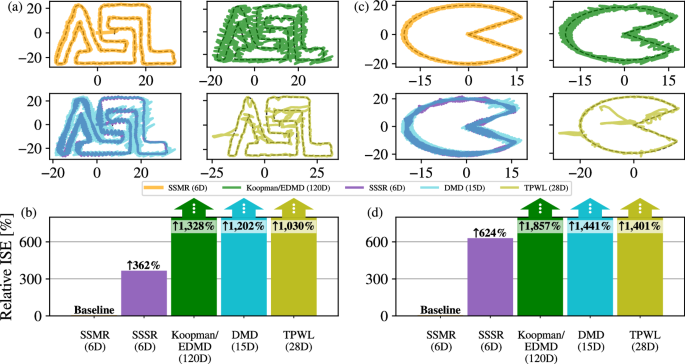
a Closed-loop trajectory for the slow ASL trajectory in the x–y plane. b Relative tracking ISE of SSMR compared to the other models for the ASL trajectory. c Closed-loop trajectory for the slow pacman trajectory in the x–y plane. d Relative tracking ISE of SSMR for the pacman trajectory. Overall, SSMR outperforms all other models with respect to tracking performance. While SSSR still outperforms all other baselines, it is performs significantly worse than SSMR due to its inability to capture the inherent geometric nonlinearities of the robot.
SSMR and SSSR consistently outperform the baseline models across all control tasks for both robots. In the case of the diamond robot, both methods effectively capture the dynamics of slow and fast trajectories, with SSMR achieving the best closed-loop performance. The performance gap between SSMR and SSSR substantially widens for the fast figure-eight task, likely due to near-resonant behavior increasing nonlinearity. For the trunk robot, SSMR models surpass all other models, including SSSR, indicating that the trunk robot’s significant geometric nonlinearities are better handled by nonlinear models. The enhanced relative performance of SSMR over SSSR across different robot morphologies and control tasks underscores the necessity for nonlinear models to improve performance in tasks that induce nonlinear behaviors.
Our results underscore two additional observations, highlighting the efficacy of our approach compared to the state-of-the-art. First, both Koopman/EDMD and DMD perform reasonably for the slow figure-eight but poorly on the fast counterpart, with Koopman/EDMD faring worse than DMD by over a factor of 20. Second, SSSR significantly outperforms both despite it extracting a simpler linear model. The former further suggests that these methods overfit to the training data, which consists of trajectories slower than the desired fast figure-eight trajectory. It is then unsurprising that Koopman/EDMD performs the worst because it has nonlinear features which pick up quasi-random variations in the data rather than learn the underlying dynamics. The latter, on the other hand, results from the fact that we are explicitly targeting resilient structures in the robots’ phase space. This allows us to uncover even linear models which generalize to control tasks well outside of its training distribution. This resilience stems from the fact that SSMs and their associated spectral subspaces persist under perturbation, e.g. due to actuation and noise35.
Trade-off between accuracy and computational complexity
To rigorously compare the models, we evaluate their performance along two dimensions: ISE and time to solve the optimal control problem. Figure 8 shows the Pareto log-plot comparing SSMR and SSSR against the baseline methods for the simulated diamond and trunk robot. Each point represents a time-discretized model in Δt = 0.02 s, which is commensurate with its control period. Since each model’s dimension is fixed, the solve time to control period ratio is the time to solve a single optimization problem divided by the time-discretization, Δt. Any model to the right of unit 1 on the solve time to control ratio axis is not real-time capable. In addition to the control tasks considered in Figs. 6, 7, we evaluate the tradeoff on an additional control task for each robot. For the diamond robot, we consider a fast circle trajectory where the diamond’s end-effector is required to track a circle in the y–z plane (e.g., see Fig. 10b). For the trunk robot, we consider the task of tracking the Stanford symbol in the x–y plane (e.g. see Fig. 10c).
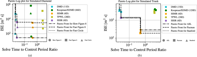
Pareto fronts for minimizing absolute ISE and MPC solve time to control period ratio for time-discretized models of Δt = 0.02 s. a Pareto Log-plot for models of the simulated diamond robot for various control tasks. While SSMR, SSSR, and DMD exhibit Pareto dominance, DMD has consistently higher ISE. b Pareto Log-plot for models of the trunk robot for various control tasks. SSMR, SSSR, and DMD are Pareto-dominant, with SSMR exhibiting the lowest ISE.
Overall, SSSR and SSMR demonstrate Pareto dominance across various robot morphologies. Both robots lie on the Pareto front, with SSMR exhibiting the lowest tracking error. While DMD also lies on the Pareto front, it has a higher ISE than both SSSR and SSMR. Koopman/EDMD and TPWL are Pareto-dominated by DMD, SSSR, and SSMR, and none of the TPWL models are real-time compatible. Although SSMR, SSSR, and DMD lie on the Pareto curve, they do not perform equally well. Generally, we aim for minimal error while maintaining real-time computation. Critically, Fig. 8 shows that with a slight increase in computation time (still real-time), SSMR and SSSR achieve superior tracking performance with reasonable qualitative behavior, as shown in Figs. 6, 7. We observe a similar tradeoff between SSMR and SSSR for the trunk robot in Fig. 8b.
While SSMR and SSSR are both 6D, the jump in computationally complexity for SSMR stems from the fact that the majority of the MPC computation for the SSMR models results from computing the Jacobians at each timestep in the MPC horizon. Fortunately, the computational complexity of SSMR-based MPC does not scale with the observables, whereas for Koopman-based MPC this complexity scales exponentially. This is seen in the trunk robot, where the number of states in the Koopman/EDMD model is more than 100 and the MPC solve time grows rapidly. The TPWL models are relatively high-dimensional for both robots, also leading to large solve times. Thus, the high computational complexity of these models result in the loss of real-time control capability, as shown in Fig. 8.
Constrained control for simulated trunk
We now compare the closed-loop performance of each model on the trunk robot in an obstacle avoidance setting to evaluate their ability to achieve precise control while remain safe. Specifically, the trunk’s tip is made to follow a 2D projection of the “ETH” symbol on the x–y plane with 20 circular obstacles at varying radii. The period of the trajectory is 10 seconds and we evaluate each model’s closed-loop tracking performance over 100 randomly generated obstacles. We consider only the single time-delayed tip positions for the SSMR model and seek to evaluate each model’s performance based on their ability to track the trajectory (i.e low RMSE) while minimizing the amount of constraint violations (i.e low violation ratio). Should it violate the constraints, the method should minimize the constraint violation (i.e low max violation).
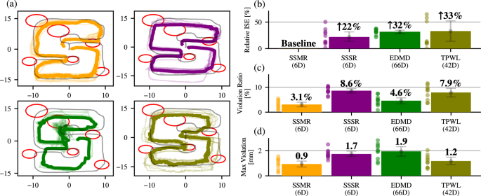
The results of this evaluation are shown in Fig. 9. The planning horizon for all models is 60 ms, which is myopic and leads to abrupt changes in the control strategy near the boundary of a constraint. Furthermore, the density of obstacles results in narrow free space, which causes these abrupt changes to happen frequently throughout the control task. These abrupt control changes result in discontinuous behavior which poses a challenge for all methods. For example, the Koopman/EDMD model fails to generalize to these behaviors, leading to erratic and unsafe behavior. While SSSR outperforms Koopman/EDMD, geometric nonlinearities induced by this trajectory coupled with the discontinuous behavior near constraint boundaries drive the linear model out of its region of validity, leading to worse performance than SSMR. Lastly, TPWL does slightly better than SSSR, likely due to its piecewise linear models providing a degree of robustness at the discontinuities.
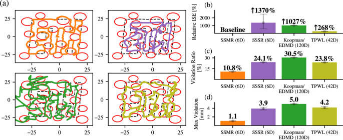
a Trajectory of most accurate tracking of “ETH” symbol among the 100 simulations for each model. b Statistics for tracking performance (ISE). c Statistics for how often the robot violated constraints (violation ratio). d Statistics for how much the robot violated the constraints (max violation). SSMR outperforms all models in terms of precision and safety.
Overall, the SSMR model effectively handles these abrupt behaviors near the constraint allowing it to outperform all other models in terms of tracking accuracy and safety. Recent results54 show that data-driven approximation of a non-smooth SSM carrying the discontinuous trajectory is justified as long as the discontinuity is moderate (i.e the two dynamical systems on both sides of the discontinuity do not differ significantly). Analogously, the SSMR procedure in Fig. 2 approximates the flow of the system on a non-smooth SSM induced by the abrupt control inputs. These results highlight that this smooth approximation is effective and useful when dealing with constraints, but compute constraints limit the planning horizon.
Hardware Experimental Validation
We now evaluate each model’s closed-loop performance on a hardware platform of the diamond robot. We expect that the hardware platform will exhibit more nonlinearity than the simulation due to unmodeled boundary conditions (e.g. imperfect fixation at the base, unmodeled friction at the interface, etc), viscoelasticity, manufacturing imperfections, and actuator hysteresis. Our experimental setup and the control tasks are shown in Fig. 10. In this evaluation, we run 10 closed-loop experiments across various tasks including a 2D figure eight in the x–y plane, a 2D Stanford symbol with obstacles in the x–y plane, and a slow circle trajectory in the y–z plane. The control frequencies for each model were chosen for real-time control: 20 Hz for the SSMR and SSSR models, 10 Hz for the Koopman/EDMD model, 50 Hz for the DMD-based LQR model, and 2.5 Hz for the TPWL model.
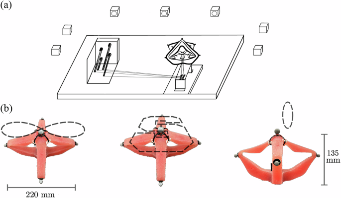
a Actuation and sensing setup for control of the real-world diamond robot. b Diamond robot and its three control tasks: (from left to right) quasi-static figure eight in x–y, “Stanford” symbol with obstacles, and quasi-static circle in y–z.
For the unconstrained figure eight and circle control tasks, we baseline against the Koopman static pregain method25, which is essentially DMD-based LQR, augmented with a feedforward control term. This method amounts to computing a linear inverse kinematic map which is used in a feedforward fashion to track a desired trajectory. Intuitively, this feedforward term controls the robot close to the reference trajectory, while the feedback term is used to correct small deviations from the trajectory. Following25, we collect training data by commanding random step inputs and partitioning them into dynamic and static components to learn the DMD model and linear feedforward term, respectively. For TPWL, we calibrate the dynamic response of the model from the finite-element simulator to align it with our hardware platform.
The results for the unconstrained control tasks are reported in Fig. 11 while those of the constrained tasks are shown in Fig. 12. Overall, SSMR outperforms all baseline models in terms of closed-loop tracking performance and safety across all the control tasks. Furthermore, although SSSR is a 6D linear model, it outperforms the more complex Koopman/EDMD and TPWL baselines in terms of tracking performance across all tasks. Despite the fact that we derive the TPWL model from a high-fidelity simulator calibrated for the real robot, its performance still suffers due to the sim-to-real gap. This highlights the appeal of data-driven methods due to their flexibility in learning the dynamics of the actual system directly from real-world data. Interestingly, while Koopman/EDMD is trained on data from the real robot, its MPC variant performs worse than TPWL in tracking performance for unconstrained tasks and comparably to TPWL for constrained tasks. This suggests that the Koopman/EDMD model overfits to the training data and does not learn the underlying dynamics of the robot. When we opt for an LQR controller and add the pregain term, DMD outperforms TPWL but falls short of our SSMR model’s performance. These results reaffirm the efficacy of our approach to learning dominant dynamics useful for real-time, predictive control.
Ten closed-loop experiments were conducted for each model. The bar plots and displayed values represent the average ISE for each model while the error bars represent 95% confidence intervals. The distribution of data points is shown to the left of each bar plot. a Qualitative performance of each model on quasi-static figure eight task in x–y. b ISE statistics of all models for figure eight trajectory. c Qualitative performance of each model on quasi-static circle task in y–z. d ISE statistics of all models for circle trajectory. Bolded trajectory represents the trajectory with best tracking performance. SSMR and SSSR outperform the baselines on both control tasks.
a Trajectory of most accurate tracking of “Stanford” symbol among the ten experiments for each model. b Statistics for tracking performance (ISE). c Statistics for how often the robot violated constraints (violation ratio). d Statistics of how much the robot violated the constraints (max violation). The bar plots and displayed values represent the average value of each metric while the error bars represent the 95% confidence interval. SSMR outperforms all models in terms of precision and safety.
Discussion
We have introduced SSMR, a data-driven methodology to model and control continuum robots. We leverage the recently developed SSM theory from dynamical systems to infer low-dimensional, yet faithful models of the robots’ dominant dynamics from numerical and experimental data. This low-dimensionality affords computational efficiency, allowing us to design an MPC scheme that provides closed-loop control in real-time while enforcing safety constraints. Using a model learning algorithm that is theoretically justified, we obtain models that are simple yet generalizable across robot morphologies and control tasks. Furthermore, our models are simple (requiring only 6-dimensions and no more than third-order polynomials) and do not require significant amounts of training data. Despite this simplicity, we demonstrate that SSMR exceeds the performance of other available data-driven modeling methods in prediction accuracy, trajectory tracking, and safety.
Our zeroth-order approximation of the time-varying SSM amounts to assuming that the desired trajectory of the robot remains close to the origin and hence, can be modeled by the SSM computed at the origin. Although the trajectories considered in the previous sections are not particularly close to the origin, this approximation still provides an SSM-reduced model that outperforms other approaches when used in MPC. The robustness of SSMR confirms that we should infer the dominant dynamics of System 1 by learning persistent attracting structures in the phase space rather than model inherently non-robust individual trajectories. While here we take a coarse approximation to minimize computational complexity, an important next step will be to efficiently compute the full SSM structure along the desired orbit up to higher orders. This will be crucial to maintaining precision during more dynamic tasks that involve larger control inputs.
Additionally, while SSMR scales independently of the number of measurements and hence allows for more complex sensor arrangements, we have simplified our study here by using only a single sensor to measure the robot’s end-effector position. Since different sets of observables might further improve the parameterization for the SSM, our future work will explore more complex sensor configurations. Another important direction for future work is addressing complex real-world dynamics, such as mechanical instabilities (e.g. buckling) and significant discontinuities like contact or fluid-structure interactions. Recent advances in SSM theory45 also apply to systems with fixed points of varying stability, offering a promising approach to controlling structural buckling. To handle discontinuities, future work can extend non-smooth SSM modeling techniques from54 and55 to enhance SSMR-based models in contact-rich environments. These controllers will be particularly useful for applications such as soft robotic fish operating in flow-disturbed environments, such as deep sea trenches (as depicted in Fig. 1d) where strong currents interact with complex geological structures.
Finally, we plan to compare our approach with methods based on first principles, such as the Cosserat rod dynamics presented in56, to further motivate the practical advantages of data-driven models.
SSMR’s flexibility coupled with its low computational cost and data efficiency makes it a promising choice for safely deploying continuum robots in high-stakes and resource-constrained environments. While the present work focuses on applications to continuum robots, our approach is independent of the specifics of the robots considered here and hence is generally applicable across robotics. Thus, we believe that our approach has the potential to enable safe and efficient control for emerging classes of autonomous systems across a spectrum of operating environments.
Methods
Spectral Submanifold theory
SSMR: Spectral Submanifold Reduction
Inspired by recent advances in nonlinear dynamics35,36,45,48, our work aims to identify the dominant dynamics of continuum robots from data for efficient model-based control. Throughout this work, we consider robots as control-affine, dynamical systems of the form
where ({bf{x}},in ,{{mathbb{R}}}^{{n}_{f}}) represents a state in the high-dimensional state space of the robot, ({bf{u}}in {{mathbb{R}}}^{m}) is the control input, ({bf{y}}in {{mathbb{R}}}^{o}) are the observed states, and Eq. (1) is locally asymptotically stable at x = 0. Note that the finite-dimensional system in Eq. (1), can be seen as the result of a spatial discretization of the underlying PDE which govern the robot’s continuum dynamics.
The success of data-driven modeling is typically attributed to the manifold hypothesis: that data sets lie along a low-dimensional submanifold, allowing for their parsimonious representation. In the context of time series, this submanifold is an attractor representing the set of states (or points in the phase space) towards which a system tends to evolve, regardless of its initial conditions. In other words, if the manifold hypothesis holds, it suggests that the dynamics of the data-generating process are confined to a low-dimensional attractor. This means that even though the time series data exist in a high-dimensional space, the process’ behavior and evolution are governed by a simpler, lower-dimensional structure. Recent results in dynamical systems confirm the existence and uniqueness of these attracting structures for dissipative systems, called Spectral Submanifolds (SSMs)35, under a set of well-defined mathematical conditions that we now review.
Consider the linearized dynamics (dot{{bf{x}}}={bf{A}}{bf{x}}) with A: = Df(0) being the Jacobian of f at x = 0 and one of its spectral subspaces,
where ({E}_{{j}_{k}}) denotes the real eigenspace corresponding to an eigenvalue ({lambda }_{{j}_{k}}) of A. Let ΛE be the set of eigenvalues related to E and Λout be the eigenvalues not related to E. If (mathop{max }nolimits_{lambda in {Lambda }_{{rm{out}}}}text{Re}(lambda ), < ,mathop{min }nolimits_{lambda in {Lambda }_{E}}text{Re},(lambda ), < ,0), then E is a slow spectral subspace corresponding to the n slowest decay modes. Based on SSM theory, for u(t) = 0, the uncontrolled System 1 admits infinitely many invariant manifolds of the same dimension as E35. These manifolds are tangent to E at the origin and attract all trajectories in the domain of attraction of x = 0 at exponential rates faster than their internal decay rates. If there are no resonances between eigenvalues in ΛE and Λout, then precisely one of those invariant manifolds is as smooth as the original dynamical System 1. The internal dynamics of this special invariant manifold serve as the de facto reduced-order model with which nearby trajectories converge to exponentially fast. This smoothest invariant manifold, denoted ({{mathcal{W}}}_{0}(E)), is called the (primary) SSM fixed to the origin of the uncontrolled system. The internal dynamics is the observed dominant dynamics of System 1 for u(t) = 0 within the domain of attraction of the origin. For typical continuum robots, the entire range of movements and configurations they are designed to perform falls within domain of attraction of ({{mathcal{W}}}_{0}(E)). The autonomous SSM, which represents the primary behavior of the uncontrolled system, effectively describes the main dynamics observed across all the robot’s intended operations.
When u(t) ≠ 0, then recent results by45 guarantee the survival of a time-dependent SSM, ({{mathcal{W}}}_{{bf{u}}(t)}(E,t)), in the controlled system, as long as either (Vert {bf{g}}({bf{x}}){bf{u}}(t)Vert) is a small perturbation to f(x) or (Vert {{bf{D}}}_{t}{bf{g}}({bf{x}}){bf{u}}(t)Vert) is small relative to (leftVert frac{d}{dt}{bf{f}}({bf{x}})rightVert). The latter condition is arguably satisfied in our setting because the intended trajectories result in control actions that do not vary faster than the time scales of the robot’s internal structural vibrations. In this setting45, calls ({{mathcal{W}}}_{{bf{u}}(t)}(E,t)) an adiabatic SSM, showing that it varies slowly along a unique anchor trajectory that has the same stability type as the uncontrolled x = 0 fixed point of System 1. In our setting, this anchor trajectory is the desired trajectory of the robot.
In the present study, we use the zeroth-order approximation (({{mathcal{W}}}_{{bf{u}}(t)}(E,t)approx {{mathcal{W}}}_{0}(E))), i.e we globally approximate the time-dependent SSM with the autonomous SSM anchored at the origin. To approximate the actual dominant dynamics within ({{mathcal{W}}}_{{bf{u}}(t)}(E,t)), we include the first-order correction to the uncontrolled dynamics, which turns out to be simply the projection of B(x)u(t) onto the spectral subspace E along the direction of fast eigenspaces outside E45. To avoid the costly identification of those fast modes, here we simply take the projection onto E to be orthogonal, as is generally assumed by the simplest variant of the SSMLearn algorithm we use here from36.
Data-driven computations of SSMs from experimental data were recently developed and successfully applied to model complex, real-world systems36,37. The practicality of these methods stem from Whitney’s embedding theorem51 which guarantees that almost all smooth maps, h, will embed an n-dimensional SSM in an o-dimensional observable space if o ≥ 2n + 1. In case we do not have enough observables, Takens’ embedding theorem52 asserts that delay-embeddings of smaller sets of measurements allow one to reconstruct the dynamics on an SSM. As long as the observables are generic49, this theorem guarantees that an n-dimensional attractor of Equation (1) can be smoothly embedded in an observable space of dimension o ≥ 2n + 1. Intuitively, this means that as long as we choose our sensor arrangement to sufficiently characterize the robots’ n mode shapes, we detect its dominant dynamics from transitions in the observables. To do this one can increase the number of sensors along the robot’s structure to obtain finer measurements of its geometric configuration. As a simplification, we only measure the x, y, and z positions of the end effectors in both the diamond and trunk robots, as shown in Fig. 2. This approach is sufficient for the considered control tasks, hence, we relegate more complex sensor arrangements to future work, as discussed in Section 3. We then take appropriate time-delayed measurements of the end-effector to achieve the dimensionality required by the Takens embedding theorem. For more details on observables and their genericity, we refer the reader to49.
SSMR for control
Combining our discussion in Section 4.1 with the SSMLearn algorithm of36, dynamics in Eq. (1) of continuum robots by learning the dynamics on the autonomous SSM anchored at the robot’s resting position. We then calibrate a control vector field which aligns these reduced dynamics with those on the time-varying SSM. Specifically, we aim to learn the parameterization map, w, and reduced dynamics, r, of the following form
where y denotes the observable vector in Eq. (1), ({bf{z}}in {{mathbb{R}}}^{n}) is the reduced coordinate vector which parameterizes the SSM, ({{mathcal{W}}}_{0}(E)), and ({{bf{z}}}^{c:{n}_{w}}) represent monomials of z from order c to order nw. The coefficient matrices ({{bf{U}}}_{n}in {{mathbb{R}}}^{otimes n}) and ({bf{W}}in {{mathbb{R}}}^{otimes q}) are the linear and nonlinear parts of the parameterization map, where (q=left(begin{array}{c}n+{n}_{w}\ nend{array}right)-n), ({{bf{U}}}_{n}^{top }{{bf{U}}}_{n}={{bf{I}}}_{ntimes n}), and ({{bf{U}}}_{n}^{top }{bf{W}}={bf{0}}). For the reduced dynamics, ({bf{R}}in {{mathbb{R}}}^{ntimes r}) is the coefficient of the drift (i.e autonomous) term, while ({{bf{b}}}_{r}:{{mathbb{R}}}^{n}to {{mathbb{R}}}^{ntimes m}) is the reduced state control input matrix. This procedure is fully data-driven and conducted with limited sensor measurements. Since the resulting model is low-dimensional, we can formulate a receding-horizon optimal control problem within ({{mathcal{W}}}_{0}(E)) (as shown in Section 4.4) which can be solved in real-time.
Specifically, we tailor our sensor arrangement, data collection, and learning algorithm to infer the unknown coefficients in Eq. (3). First, we arrange sensors on the robot so that our observable measurements are generic49 and produce feature-rich training data. Intuitively, genericity suggests that choosing a comprehensive sensor arrangement capable of detecting the robots’ primary modes which span its expected operating configurations enables us to accurately model the SSM and its dynamics.
We then collect two training datasets: one consists of decaying trajectories from a collection of initial conditions, denoted Y, and the other consists of controlled trajectories, denoted Yu. To learn an approximation of the dominant dynamics, we follow a three-step process.
-
1.
We conduct SVD on the decaying trajectory dataset, ({bf{Y}}in {{mathbb{R}}}^{otimes {N}_{{rm{traj}}}}), to approximate the tangent space of the SSM i.e
$${bf{Y}}={bf{U}}{mathbf{Sigma }}{{bf{V}}}^{top },$$(4)where Ntraj represents the number of training trajectories and Un represents the leading n columns of U, which are a good estimate of the tangent space of the n-dimensional SSM49.
-
2.
To infer the unknown coefficients in the parameterization and autonomous dynamics of the SSM in Eq. (3), we solve the optimization problems
$$begin{array}{l}{bf{W}},=arg mathop{min }limits_{{bf{W}}}leftVert {bf{Y}}-{{bf{U}}}_{n}{bf{Z}}-{bf{W}}{{bf{Z}}}^{2:{n}_{w}}rightVert ,\ {bf{R}};,=arg mathop{min }limits_{{bf{R}}}leftVert dot{{bf{Z}}}-{bf{R}}{{bf{Z}}}^{1:{n}_{r}}rightVert ,end{array}$$(5)where ({bf{Z}}={{bf{U}}}_{n}^{top }{bf{Y}}) encodes the training decay data matrix into reduced coordinates and the derivatives are comuted via numerical differentiation.
-
3.
We approximate the dominant dynamics on the approximating SSM, ({{mathcal{W}}}_{0}(E)), via calibration that amends the autonomous SSM dynamics learned from decaying trajectories with the time-varying SSM dynamics of the controlled system. If br(z) is a smooth function of z, then this calibration amounts to solving the optimization problem
$$({bf{B}},{{bf{B}}}_{r})=arg mathop{min }limits_{{bf{B}},{{bf{B}}}_{r}}{leftVert {dot{{bf{Z}}}}_{{rm{u}}}-{bf{R}}{{bf{Z}}}_{{rm{u}}}^{1:{n}_{r}}-{bf{B}}{bf{U}}-{{bf{B}}}_{r}{{bf{Z}}}_{{rm{u}}}^{1:{n}_{u}},{otimes }_{c},{bf{U}}rightVert }_{F}^{2}.$$(6)Here, ({bf{X}},{otimes }_{c},{bf{U}}:=left[{{bf{X}}}_{cdot ,1}otimes {{bf{U}}}_{cdot ,1},ldots ,{{bf{X}}}_{cdot ,N}otimes {{bf{U}}}_{cdot ,N}right]) is the Kronecker product applied columnwise, ({{bf{Z}}}_{u}={{bf{U}}}_{n}^{top }{{bf{Y}}}_{u}) encodes the controlled training data matrix into reduced coordinates, and the control vector field is given by
$${{bf{b}}}_{bf{r}}({bf{z}})({bf{u}}),:!={bf{B}}{bf{u}}+{{bf{B}}}_{r}left({{bf{z}}}^{1:{n}_{u}}otimes {bf{u}}right).$$(7)
Our SSMR algorithm operates under the assumption that the control effort is sufficiently small, allowing the leading-order component tangential to the SSM to serve as an adequate approximation. In practice, we observe that the excitation of outer modes due to orthogonal control components lead to fast transients back to the manifold. Thus, the effect of excited external modes are short lived and our approximation is justified.
Reparameterizing the SSM for control
We avoid excessive time delays in the control loop by reparameterizing the SSM with a different set of control observables, thereby mitigating the curse of delays. At a high level, we detect the dominant dynamics from sufficiently time-delayed decay data, then embed the SSM in our chosen control observable space. In this section, we simplify notation by reusing the variable y to refer to our new control observable.
To detect the dominant dynamics, we first need to embed the SSM in an appropriate observable space. By following Step 1 in Section 4.2, we obtain a projection onto the reduced coordinates, z, which parameterizes the SSM within the observable space. This allows us to infer reduced coordinates whose dynamics approximate the dominant dynamics. These reduced coordinates are valid because the SSM is guaranteed to be embedded in ({{mathbb{R}}}^{o}) and SVD of the observables’ decaying trajectories in this space is a good approximation of the SSM’s spectral subspace. To avoid the curse of delays, we then reparameterize the SSM in the new observable space, by finding a parameterization map, ({bf{w}}:{{mathbb{R}}}^{n}to {{mathbb{R}}}^{p}), and chart map, ({bf{v}}:{{mathbb{R}}}^{p}to {{mathbb{R}}}^{n}), commensurate with our control observable, ({bf{y}}in {{mathbb{R}}}^{p}),
such that v ∘ w = In × n and p ≥ n. Since we have inferred valid reduced coordinates, fitting a parameterization map of the SSM on an observable space, ({{mathbb{R}}}^{p}), of at least the same dimension as the SSM is theoretically justified.
Given the decay data matrix in reduced coordinates, Z obtained from Step 1 in Section 4.2, we parameterize to the new observables by solving the following optimization problem
where our chart map is given by ({bf{z}}={bf{v}}({bf{y}})={{bf{V}}}_{n}^{top }{bf{y}}). We then carry out Steps 2 and 3 in Section 4.2 to obtain our control-calibrated reduced dynamics, which we can then use for efficient control synthesis. To solve the constrained optimization problem in Eq. (9), we restrict Vn to lie on the Steifel manifold of orthonormal matrices57. We can then use existing software packages58,59 to numerically solve for the unknown coefficients.
In this work, we adopt a simpler approach, bypassing the need to formulate a manifold optimization problem. Let us denote (bar{{bf{z}}}in {{mathbb{R}}}^{n}) as the reduced coordinates inferred from decaying trajectories of the potentially many time delayed measurements in ({{mathbb{R}}}^{o}).
-
1.
We fit a parameterization map between our new control observable y and (bar{{bf{z}}}) by solving the following unconstrained problem
$${bar{{bf{V}}}}_{n},bar{{bf{W}}}=arg mathop{min }limits_{{bar{{bf{V}}}}_{n},bar{{bf{W}}}}leftVert {bf{Y}}-{bar{{bf{V}}}}_{n}bar{{bf{Z}}}-bar{{bf{W}}}{bar{{bf{Z}}}}^{2:{n}_{w}}rightVert ,$$(10)where Y is the decay data matrix of the new control observables and (bar{{bf{Z}}}) is the reduced coordinate data matrix computed in Step 1 of Section 4.2.
-
2.
Since Eq. (10) is unconstrained, ({bar{{bf{V}}}}_{n}) need not be orthonormal. Thus, we scale and rotate (bar{{bf{Z}}}) to obtain the new reduced coordinates ({bf{Z}}={{bf{V}}}_{n}^{top }{bar{{bf{V}}}}_{n}bar{{bf{Z}}}), where the orthonormal matrix ({{bf{V}}}_{n}in {{mathbb{R}}}^{ntimes p}) is obtained by orthonormalizing ({bar{{bf{V}}}}_{n}) via Gram-Schmidt and defines the chart map, v, in Eq. (8).
-
3.
This chart map allows us to define a graph-style parameterization between the new reduced coordinates, z and the control observables, y, satisfying the orthogonality constraints in Eq. (9). Specifically, we solve another unconstrained optimization problem
$${{bf{V}}}_{n},{bf{W}}=arg mathop{min }limits_{{{bf{V}}}_{n},{bf{W}}}leftVert {bf{Y}}-{{bf{V}}}_{n}{bf{Z}}-{bf{W}}{{bf{Z}}}^{2:{n}_{w}}rightVert ,$$(11)where ({{bf{V}}}_{n}^{top }{{bf{V}}}_{n}={{bf{I}}}_{ntimes n}). The solved coefficients define the parameterization map, w, in Eq. (8) between the reduced coordinates and our control observable.
We complete the procedure by conducting Steps 2 and 3 in Section 4.2 to fit the calibrated reduced dynamics in the new reduced coordinates, z. By using this reparameterization trick, we can approximate the dominant dynamics while overcoming the curse of delays during control operation.
SSMR-based model predictive control
Model predictive control (MPC) is a modern control strategy based on optimization that has widespread applications in both industry and academic settings. Its core concept involves continuously solving finite-horizon, open-loop control problems in real-time. Feedback is implicitly generated through the application of the initial segment of the optimized control sequence, followed by the repetition of the real-time optimization process at subsequent time steps. The advantages of MPC are threefold: (1) optimization of performance criteria; (2) handles state and input constraints; (3) applicable to general nonlinear systems.
MPC is amenable for precise, real-time control when the prediction model is accurate and sufficiently low-dimensional. By approximating the dominant dynamics of Eq. (1), SSMR generates faithful, low-dimensional models that enable real-time MPC designs. To design the MPC, we discretize Eq. (3) in time and, with slight abuse of notation, formulate the optimal control problem,
where ({hat{{bf{y}}}}_{k}) is the reference state at time k, (Nin {mathbb{Z}}) is the prediction horizon, Q, Qf are positive semi-definite matrices which represent the observed state and terminal costs, while R is a positive-definite matrix that penalizes control input. The sets ({mathcal{Y}}) and ({mathcal{U}}) represent state and input constraints, respectively, that are potentially non-convex.
Intuitively, our MPC makes predictions on the approximated, low-dimensional SSM. It first infers the reduced state, zk, from the observed state, yk, at each time-step k via a state estimation step. Then, it predicts the evolution of the system in the reduced space (i.e tangent space) over the next N time-steps, and maps back to the approximate manifold to obtain the observables’ evolution. While (12) is non-convex, we use sequential convex programming (SCP) to transform the MPC into a sequence of quadratic programs, which is solved iteratively until convergence. While SCP has been shown to be useful in for nonlinear MPC, the computational burden of computing Jacobians at each solve step necessitates low-dimensional models. Fortunately, the reduced states in SSMR are low-dimensional, making (3) possible to solve in real-time. Our SSMR-based MPC scheme is outlined in Fig. 2c.


Responses