Diversity of biomass usage pathways to achieve emissions targets in the European energy system

Biomass is a diverse and versatile renewable energy source that can be used for various purposes^1,2,3. In the electricity system, it can complement the variable renewable energy (VRE) sources of solar and wind power^4,5,6,7 and provide dispatchable (firm) generation to meet demand even in periods of supply shortage in a VRE-based energy system^8,9. If used for combined heat and power (CHP), it can provide flexible energy, which may be especially important during so called cold–dark doldrums, when space heat demand is high and electricity supply from wind and solar is low^10,11. Biomass can also supply hydrocarbons to sectors that are challenging to electrify and where renewable alternatives are scarce, such as aviation and marine transport^12,13,14, or plastics and high-value chemicals^15,16,17. Also, it can be used to provide process heat for industry^18,19. All of these options can to some extent be combined with carbon capture (BECC) to provide carbon for further usage (BECCU), or negative emissions through geological sequestration (BECCS)^4,6,18,19. In contrast to direct air capture (DAC), which requires a substantial electricity and heat input to extract CO₂ from the atmosphere²⁰, BECC captures more concentrated CO₂ in exhaust and waste streams and provides net energy output along with the carbon capture.

The European Union and United Kingdom have adopted targets of net-zero greenhouse gas (GHG) emissions for all sectors to comply with the Paris Agreement targets^21,22. To achieve such targets, residual emissions, such as methane emissions in agriculture, need to be offset by carbon dioxide removal (CDR) from the atmosphere, where BECCS and DACCS emerge as key options for technical CDR^23,24,25.

Biomass is a limited resource and its use for energy can be associated with a range of positive and negative environmental, social and economic effects that are context specific and depend on land type and climatic region, prior land use and how bioenergy feedstock and management regimes are shaped^{26,27,28,29,30,31,32,33}. Due to concerns about possible environmental impacts, insufficient emissions reductions and competition with the food sector, EU policy has capped biofuels from food and feed crops and increasingly emphasizes lignocellulosic biomass, especially residues and waste^34,35, and prioritizes the biomass usage to energy applications where other alternatives are currently difficult to find or considered to be too costly.

All of the possible biomass usage options face competition from electricity-derived energy carriers and fossil fuels (Extended Data Fig. 1). A full systems analysis of biomass allocation to different energy uses therefore requires broad coverage of options and sectors. Such analyses have been carried out with global integrated assessment models (IAMs), with a large variety in results, but with biomass in the longer term generally ending up being used for electricity and/or liquid fuels production³⁶, coupled with carbon capture and storage (CCS)^37,38. The potential value of negative emissions from BECCS has been found to be very high, enabling the achievement of more ambitious climate targets^37,39,40,41 or delayed phase-out of fossil fuels if temperature overshoot is permitted^40,41. The latter raises concerns over risks in relying on future technology deployment to compensate for earlier emissions and over intergenerational equity^42,43,44,45.

However, IAMs lack the spatio-temporal detail needed to capture the variability of, for instance, VRE and electrolysis, and the interplay of these technologies with biomass options, such as dispatchable bioelectricity. In addition, the costs of VRE have often been overestimated in IAM-based analyses^46,47 and carbon sequestration capacities may be more limited than what has been assumed^48,49; both of these factors risk exaggerating the role of CCS for meeting climate targets^48,50. Moreover, IAMs have until now not included carbon capture and utilization (CCU) or electrofuels^11,47, leaving biofuels as the only non-fossil-fuel option, and until recently also not included DAC as an alternative CDR option^47,51,52. Most or all of these limitations apply also to previous IAM analyses focusing specifically on biomass and/or BECCS^{36,37,39,40,41,53,54,55,56,57,58,59}, leading to potential biases in the cost effectiveness of biomass usage, BECCS and different biomass utilization pathways.

Energy system models (ESMs) on the other hand commonly represent VRE explicitly, with a high spatial and temporal resolution, and some ESMs have recently been enhanced to encompass all energy sectors simultaneously^60,61. This enables a sector-coupled analysis of biomass usage for energy across all sectors and of interactions with competing fuel options that can be produced from VRE sources, such as hydrogen and electrofuels. However these models usually include a restricted selection of biomass applications and, in contrast to IAMs, only a few studies based on sector-coupled ESMs have focused explicitly on biomass, bioenergy and/or BECC^11,62, and a thorough assessment of biomass usage including BECCUS across usage options is still lacking. Further, combining bioenergy processes with conventional carbon capture results in higher costs for the additional capture and heat infrastructure and energy penalties to provide the substantial process heat needed to regenerate solvents. Such details have, to date, not been included in analyses with sector-coupled ESMs but are also lacking in many IAMs (Extended Data Table 1).

IAM and ESM studies commonly focus on the single cost-optimal solution, complemented with some sensitivity analyses. However, social planning projects are subject to a plurality of economic and socio-political objectives^63,64, and uncertainties and objectively irreconcilable trade-offs at different levels regarding future energy systems⁶⁵ and biomass use^66,67,68 are so-called wicked facets of their planning⁶⁹. The sector-coupled energy system involves diverse stakeholders with conflicting non-economic objectives and risk perceptions, and past energy transitions have been found not to follow cost-optimal paths in hindsight⁷⁰. There is therefore a value in exploring the diversity of near-optimal solutions for the energy system in general and for biomass usage in particular, to provide insights for policy about the flexibility of solutions⁷¹. Recent analyses have shown that the technology mix variety of near-optimal solutions, when allowing a small system cost increase, can be distinctly different from the single least-cost solution, in heat supply⁷², the power system^73,74,75,76, in integrated assessments⁷⁷ and in a sector-coupled European energy system^61,64. The available amount of biomass has been found to affect the manoeuvring space substantially⁶¹, calling for a thorough assessment of near-optimal solution spaces for biomass usage in the energy system. Also, whereas net-negative emissions trajectories have been assessed widely with IAMs, few net-negative analyses have been performed with ESMs^11,78.

This study addresses this gap by using a sector-coupled ESM, with a more comprehensive coverage of bioenergy technologies and BECC than in similar modelling studies (Extended Data Table 1). The overarching goal of the study is to analyse effects on the system cost of broad ranges of biomass supply and biomass technology deployment in a European energy system adhering to stringent emissions targets. This is done through a detailed exploration of the near-optimal solution space for biomass usage options, within the sector-coupled European energy system optimization model PyPSA-Eur-Sec. The effects of different deployment levels for wind power, solar PV and electrolysers on biomass usage, and vice versa, are also assessed. More specifically, we analyse the solution space around the least-cost optimum, for system cost increases of 1%, 5%, 10%, through to 25%.

Scenarios with net-negative (−110%) and net-zero CO₂ emissions compared with 1990 levels are assessed. No explicit target year is modelled, as focus is on how these targets can be met cost effectively, rather than on pathways leading there. European policies prioritize emissions reductions over compensation of emissions through CDR^{22,44,79,80,81,82}. Also, although theoretical geological storage capacities are vast, investable potentials and CO₂ injection rates as indicated by historical fossil extraction may be limited⁴⁸. Reflecting these aspects, in the main scenarios, we assess an energy system where only very little compensation of concurrent fossil fuel usage through negative emissions is permissible by setting carbon sequestration capacities near the limit for what is necessary to achieve the respective emissions targets, while also offsetting process emissions considered to be unavoidable, for instance, from cement production (Extended Data Fig. 2; 600 Mt CO₂ per year for net-negative (−110%) and 140 Mt CO₂ per year for net-zero, thus allowing the same slack for fossil fuel usage in both cases). The effect of higher assumed carbon sequestration capacities is analysed and discussed in a sensitivity analysis.

Reflecting current EU policy direction, bioenergy feedstock is assumed to consist of residues, with a domestic supply potential corresponding to the medium level in the JRC ENSPRESO database⁸³. Import of non-digestible biomass represents a complementary, but more expensive, feedstock source¹¹ (Extended Data Fig. 3). The effect of variations to these assumptions is assessed in sensitivity analyses.

We find that provision of biogenic carbon for negative emissions and utilization has a higher value than bioenergy provision. Energy system costs increase by 20% if biomass is excluded at a net-negative (−110%) emissions target. Dispatchable bioelectricity covering ~1% of total electricity generation strengthens supply reliability. Otherwise, it matters less whether biomass is used for combined heat and power, liquid fuel production or industrial process heat, as long as the carbon content is utilized to a high extent, as facilitated through carbon capture to provide renewable carbon for negative emissions or for production of fuels for further use in the energy system.

In the cost-optimal solution for the net-negative scenario, wind (54%), solar photovoltaics (PV) (40%) and hydropower (5%) supply 99% of the whole electricity demand at 9,250 TWh (Extended Data Fig. 4), which is almost three times the electricity demand in 2021^84,85. Biomass is mainly used to complement the supply of fuels and chemicals for industry, aviation and shipping, but a small share is also used to supply dispatchable electricity (Extended Data Fig. 4). Some 637 TWh biogas and 2,896 TWh solid biomass (2,172 TWh imported) are used, corresponding to 29% of the annual primary energy consumption at 13 PWh. Solid biomass usage amounts to about two times the 1,290 TWh used in 2021, when overall bioenergy usage was at 1,937 TWh (refs. ^84,85). Around 87% of biomass usage is combined with carbon capture, with the exception being dispatchable biomethane applications. The total annual system cost amounts to €822 billion.

If overall biomass usage is restricted to current usage levels, the system cost ends up ~5% higher than without restrictions. If all biomass (except mandatory incineration of municipal solid waste) is excluded, it leads to a 20% higher system cost (Fig. 1a), or an additional cost of €169 billion annually, roughly corresponding to European defence expenses⁸⁶. This is twice as much as the cost of excluding solar power and similar to the cost of excluding wind power, despite both of them cost optimally providing more primary energy (Fig. 2d,e). Excluding any of these primary energy sources thus leads to much higher costs. Wind and solar power are more readily interchangeable whereas the substitution of biomass is much more expensive because biomass provides non-fossil carbon in addition to energy, for which the substitute, DAC, coupled with a necessary expansion of additional energy provision, ends up much more expensive. Wind and solar power cannot be excluded simultaneously even at a 25% system cost increase (Fig. 2f).

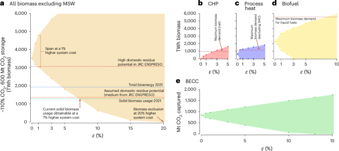
The respective options are minimized and maximized to map out the space of feasible solutions (shaded area) for a given allowed system cost increase ε (percent deviation from the total system cost). a,e, The solution space when varying the amount of biomass (except municipal solid waste) (a) and the solution space when varying bioenergy with carbon capture deployment (e). In a, solid biomass usage in 2021^84,85 is shown and is similar to the assumed medium domestic residue potential, in contrast to the high potential, both from JRC ENSPRESO⁸³. Total bioenergy in 2021^84,85 includes biomass residues and agricultural crops. b–d, Horizontal lines show biomass demands if the full demand for district heat (b), industrial process heat (c) and liquid fuels (d) would be fulfilled by solid biomass. The heat demand for CHP can be expanded to supply thermal storage and the industrial process heat demand can be used to supply DAC heat demand. MSW, incineration of municipal solid waste, which is set to be compulsory.

Full size image

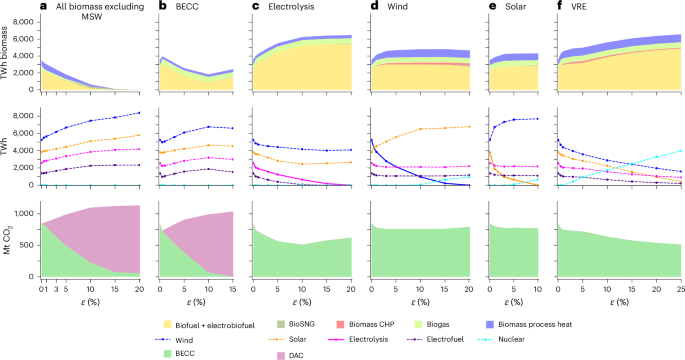
Upper panels show biomass usage (TWh biomass), the middle panels show other energy technologies (TWh) and the lower panels show carbon capture (Mt CO₂ for BECC (bioenergy with carbon capture) and DAC (direct air carbon capture)). a, For example, total biomass (excluding mandatory waste incineration) is the objective function, which is minimized. In the upper panel the effect on biomass usage can be observed as total biomass use decreases. In the middle panel the effect on other energy technologies such as wind power can be observed as total biomass use decreases, and in the lower panel the effect on carbon capture is shown. b–e, BECC is minimized as shown in the lower panel (b), whereas for electrolysis (c), wind power (d) and solar PV (e), the minimized technology is shown as a solid line in the middle panels. f, The results when minimizing variable renewables (solar PV and wind power). BioSNG, biogenic synthetic natural gas.

Full size image

The assumed biomass availability determines both relative and absolute costs of excluding biomass. If biomass imports are not included as an option, excluding biomass altogether results in a 9% higher system cost. If the high domestic residue potential estimate from JRC ENSPRESO is used instead of the medium potential, and biomass imports are included as an option, the system cost increases 29% when excluding biomass altogether. Excluding biomass imports results in substantially higher solid biomass and CO₂ prices (Table 1), indicating a high system pressure for increasing biomass supply.

Substantial flexible dispatchable methane-based power capacities emerge in the net-negative scenario (521 GW_el open-cycle gas turbines and gas CHPs), on par with the inflexible electricity demand peak of 526 GW (base-load household, commercial and industrial electricity demand, excluding heat). This flexible power capacity is seldom used, with capacity factors of 28% (Fig. 3), which renders the addition of costly carbon capture to these power plants prohibitively expensive. For carbon capture to be cost effective for a particular technology, high utilization rates are needed due to the high investment cost of the additional infrastructure.

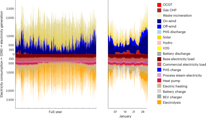
Electricity generation and consumption for achieving net-negative (−110%) emissions over the full year and for January. 521 GW_el dispatchable firm generation capacity emerges (open-cycle gas turbines (OCGT) and gas CHPs), on par with the inflexible electricity demand peak of 526 GW (base-load household, commercial and industrial electricity demand, excluding heat), but capacity factors are low, at 2% and 8%, respectively. Electricity generation and consumption are shown above and below the zero line, respectively. BEV, battery electric vehicle; PHS, pumped hydro storage; V2G, vehicle-to-grid.

Full size image

Although only 225 TWh (bio)methane is used to flexibly supplement variable renewable electricity supply (covering 1% of total generation), this option is the most costly to replace and remains longest when biomass usage is minimized (Fig. 2a). Different to studies limited to the power system only, which indicate a substantially larger firm generation energy requirement⁸, or IAM studies, which often obtain substantial biomass use for electricity production³⁶, this study finds lower levels of bioelectricity use because the sector-coupled model entails large flexible demand capacities such as electrolysers, heat storage, batteries and electric vehicles, which handle most of the variability in the power system and thus support high VRE shares (Fig. 3).

System flexibility from sector coupling, energy storage and transmission reduces the dependency on biomass. With lower assumed flexibility, the system cost of excluding biomass increases from 20% to 23% (Table 1). Similar amounts of biomass are used for flexible bioelectricity, but least-cost biomass usage shifts from fuel production to heat generation.

Excluding biomass in the net-zero scenario increases system costs by 14%, substantially less than the 20% increase in the net-negative scenario. The cost-optimal biomass use (Fig. 4) is 36% lower than in the net-negative scenario and within the range of the European Commission net-zero scenarios (2,200–2,900 TWh) (ref. ⁸⁷). Biomass usage is still cost optimally coupled with carbon capture, and solution spaces for individual options are rather similar to the net-negative scenario.

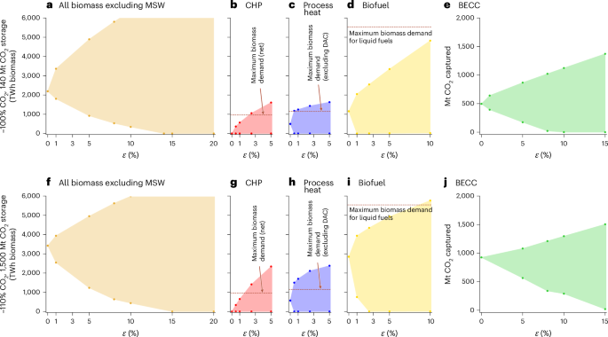
a–e, In a net-zero scenario with carbon sequestration capacity set to 140 Mt CO₂ per year, close to what is necessary to achieve the target (a–e), and a net-negative (−110%) emissions scenarios with an allowed carbon sequestration potential of 1,500 Mt CO₂ per year (900 Mt CO₂ per year more than in the base case) (f–i). The respective options are minimized and maximized to map out the space of feasible solutions (shaded area) for a given allowed system cost increase ε (percent deviation from the least-cost objective value). a,f, Solution spaces when varying the amount of biomass (except municipal solid waste) in the net-zero scenario (a) and in the net-negative scenario with higher carbon sequestration potential (f). b,g, Solution spaces when varying solid biomass use for combined heat and power in the net-zero (b) and net-negative (g) scenarios. c,h, Solution spaces when varying solid biomass use for industrial process heat in the net-zero (c) and net-negative (h) scenarios. d,i, Solution spaces when varying solid biomass use for liquid fuel and chemical production in the net-zero (d) and net-negative (i) scenarios. e,j, Solution spaces when varying bioenergy with carbon capture deployment in the net-zero (e) and net-negative (j) scenarios. b–d,g–i, Horizontal lines show biomass demands if the full demand for district heat (b,g), industrial process heat (c,h) and liquid fuels (d,i) would be fulfilled by solid biomass. The heat demand for CHP can be expanded to supply thermal storage, and the industrial process heat demand can be used to supply DAC heat demand.

Full size image

For the net-negative scenario, 87% of biomass use is cost optimally combined with carbon capture, providing 0.84 Gt biogenic CO₂ annually, corresponding to ~21% of total regional GHG emissions in 2021, at 4 Gt CO₂-equivalent (ref. ⁸⁸). The captured amount falls within projected feasible CCS growth already for 2040, of 1–4.3 Gt per year globally⁴⁹, but would require a ramp-up of BECC from currently near-zero commercial capacity to covering almost all biomass conversion.

Renewable carbon provision is the key system service of biomass, more so than the energy provided. The only other alternative for non-fossil carbon provision is DAC, which is substantially less cost competitive than the available alternative energy provision options. The value of biogenic carbon is estimated to be up to over three times higher than the value of the primary energy provision at low biomass usage levels in a renewable energy system, in both the net-negative (Fig. 5a) and net-zero scenarios (Fig. 5c). When a higher carbon sequestration allowance permits a larger amount of fossil fuels to be offset by the sequestration of biogenic CO₂, the value of the biogenic carbon is up to two times higher (Fig. 5b). With varying amounts of biomass in the system, CO₂ and solid biomass prices are strongly and similarly affected, whereas the hydrogen price is substantially less affected.

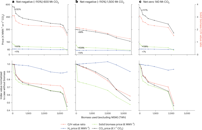
H₂ is assumed as the reference for biomass energy, with prices consumption weighted over all regions and time steps. Upper panels show resulting shadow prices (left y axis) and the carbon/hydrogen value ratio of solid biomass (right y axis). Lower panels show the prices normalized to the value when biomass is excluded. a,b, Net-negative (−110%) scenarios with carbon sequestration capacity limited to 600 (a) and 1,500 Mt CO₂ (b). c, A net-zero scenario with carbon sequestration capacity limited to 140 Mt CO₂. Solid biomass is assumed to generate 0.3667 t CO₂ MWh⁻¹ at combustion.

Full size image

BECC can be excluded at a 13% system cost increase (Fig. 1e), with mainly biofuel production decreasing whereas biogas and biomass usage for process heat and flexible bioelectricity remain cost effective also without BECC (Fig. 2b). If BECC is removed, biomass can be excluded within a 6% cost increase (Table 1), substantially less than with BECC. Capturing biogenic CO₂ emissions enhances carbon utilization, enabling scarce renewable carbon to be used multiple times and to provide negative emissions. As BECC is decreased, biomass usage also decreases, and DAC increases to provide both the necessary negative emissions and carbon for the production of electrofuels, resulting in higher total carbon capture deployment (Fig. 2b).

In the least-cost case, the shadow price (marginal price of an additional MWh) of solid biomass amounts to €54 MWh⁻¹ (as determined by the import biomass price) and €135 MWh⁻¹ if biomass is excluded (Fig. 5a and Table 1). This is substantially higher than the cost of domestic residue supply (Extended Data Fig. 3 and Extended Data Table 2) or 2020 wood chip prices at €20–25 MWh⁻¹ (ref. ⁸⁹). The resulting CO₂ price (marginal cost of CO₂ emissions) amounts to ~€260 t⁻¹ CO₂ in the cost-optimal case but increases to €591 t⁻¹ CO₂ if biomass is excluded (Fig. 5a and Table 1), indicating a high value of biomass resources to achieve emissions targets.

Solid biomass is cost optimally used for biofuel production and process heat (Extended Data Fig. 4), but a large range of near-optimal solutions for different usage options exist (Fig. 1b–d). Thus, even though it is costly to exclude overall biomass usage, it is not so important in which sectors biomass is used.

District heat is cost optimally covered by a mix of excess heat from biofuel production and electrolysers, waste incineration, electric boilers and some (bio)methane-fuelled CHP (Extended Data Fig. 4). Whereas absent in the cost-optimal solution, solid biomass CHP can cover up to 50% of district heat demand within a 1% system cost increase (corresponding to 16% of district heat cost and thus not increasing the sectoral costs substantially; Fig. 1b). These CHP plants are invariably equipped with carbon capture, which increases capital cost substantially (Extended Data Table 1), and they are therefore run with high capacity factors (>90%), coupled with heat storage, highlighting the priority of carbon capture over additional variation management supporting wind and solar feed-in.

Solid biomass competes with hydrogen and (bio)methane for process heat supply in the medium-temperature range and mainly with electricity for process steam production. It can cover a span of 0–100% in these sub-sectors within the range of a 0.5% system cost increase (7% of costs in these sectors; Fig. 1c). Thus, a very diverse set of alternative options exists within a small cost span.

Biofuels cover a span of 20–61% of liquid fuel demand for aviation, shipping and chemicals already within the range of a 1% system cost increase (Fig. 1d). A wide near-optimal range for fuel supply appears: direct biomass usage for liquid fuel production can be excluded at a 3% system cost increase (8% of liquid fuel supply cost), while covering the full liquid fuel demand with only biofuels can be done at an 8% system cost increase (resulting in more than a doubling of biomass imports).

When biomass use is decreased from the cost-optimal amount, the primary change occurs in the production of liquids used as fuels in aviation and shipping and as feedstock for chemicals, where bioliquids are replaced by electrofuels. Electricity generation from wind and solar power increases more than the usage of bioenergy decreases due to the increasing electricity demand for electrolysis and DAC to supply hydrogen and carbon for electrofuel production (Fig. 2a).

The cost-optimal results depend on a large expansion of solar and onshore wind power and even more so if biomass is excluded (Fig. 2a and Extended Data Table 3). Achieving these VRE capacities requires an unprecedented capacity growth at the European scale, which might be hindered, for instance, by industry scale-up inertia and local opposition where wind and solar projects are planned^{5,90,91,92,93,94}. When VRE is restricted to a level below the least-cost case, a decrease in total electricity generation and hydrogen electrolysis to supply electrofuel production is observed, whereas biomass use increases to supply more biofuel production and process heat (Fig. 2f).

Results also depend on a large capacity expansion of hydrogen electrolysis, which similarly requires an unprecedented scale-up (Extended Data Table 3). The cost-optimal electrolysis capacity is more than two times projected feasible capacity growth by 2050 for the European Union and covering a substantial share of projected global capacities⁹⁵ and again even more so if biomass is excluded (Extended Data Table 3). Decreasing electrolysis from cost-optimal levels leads to a corresponding reduction in electricity consumption and a decrease in electrofuel production, which is again balanced by an expansion of biomass use to supply biofuel production. Electrolysis can be excluded at an ~20% system cost increase, at which point biomass use is almost doubled compared to cost-optimal levels (Fig. 2c). A similar magnitude of biomass usage emerges when VRE is minimized within the same system cost increase (Fig. 2f).

Thus VRE or electrolyser expansion inertia primarily affects liquid fuel supply and leads to a much higher demand for biomass if emission targets are to be achieved. Vice versa, a shortage of biomass increases the value of electrofuels.

Domestic biomass resources are limited to residues, which have a lower risk of indirect emissions compared to dedicated energy crops, but residue extraction can cause soil carbon losses and impact soil health^{96,97,98,99,100}, which in turn can impact yield levels, potentially leading to indirect emissions if production is expanded elsewhere to compensate for declining harvest levels. In addition, biomass imported into Europe may be associated with GHG emissions along the supply chain.

European policies can restrict imports of high GHG biomass and require domestic residue extraction to follow best-management practices to minimize soil impacts. Supply chain emissions can be expected to decrease if other regions also adopt stringent emissions targets, and residual emissions can be offset through CDR. However, whereas innovation and changes in land-management practices can lead to dramatic emissions reductions, implementation may be a multi-decadal process^{23,101,102,103,104} and biomass supply may still be associated with emissions due to weak compliance and leakage effects^105,106. Furthermore, CDR implementation could offset emissions associated with other activities if it is not needed to offset residual emissions from the biomass supply chain.

Assuming biomass imports to entail upstream emissions can have a strong influence on biomass usage in the energy system, depending on the assumed allowed carbon sequestration potential (Fig 6). A higher allowed annual carbon sequestration potential beyond the restrictive 600 Mt CO₂ per year limit results in similar but somewhat wider solution spaces for all biomass usage options (Fig. 4), as there is room for using more fossil fuels if emissions are captured and stored or counterbalanced by negative emissions.

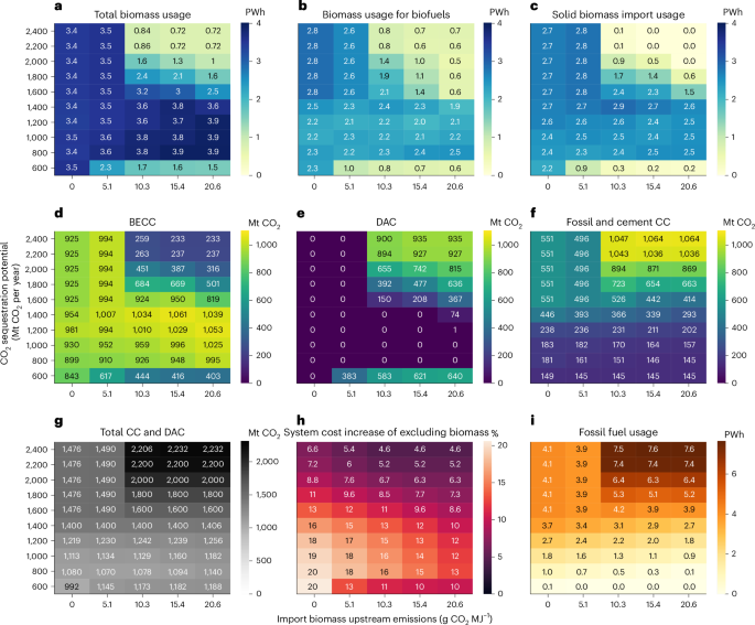
Heat maps show cost-optimal configurations for achieving a net-negative (−110%) emissions target when varying upstream emissions of biomass imports (x axis) and allowed annual carbon sequestration potentials (y axis). Upstream emissions equivalent to 10% of the biomass CO₂ emissions at full combustion corresponds to 10.3 g CO₂ MJ⁻¹. For reference, estimated nitrous oxide emissions from fertilization correspond to 0.4–14 g CO₂equivalent MJ⁻¹ for poplar or willow depending on yields and soil conditions, and, for example, substantially more for rape seed¹⁴⁷. Fossil fuels in this analysis are not assumed to entail upstream emissions, which presents an optimistic case for their performance. a,c, Total (a) and imported (c) biomass usage. b, Biomass usage for biofuels. d–g, Least-cost deployment of BECC (d), DAC (e), fossil and cement carbon capture (CC) (f) and total carbon capture and DAC (g). h, The system cost increase of excluding biomass (except municipal solid waste) compared to the least-cost solution for all combinations of carbon sequestration capacity and upstream emissions of biomass imports. i, Fossil fuel usage.

Full size image

If biomass imports are assumed to be carbon neutral (that is, without upstream emissions), least-cost biomass usage amounts are stable across a wide range of carbon sequestration allowances (Fig. 6a). However, the cost to exclude biomass decreases substantially with increasing allowed carbon sequestration potential (Fig. 6h), as it opens up for using fossil fuels (Fig. 6i) combined with CCS, which decreases the cost effectiveness of CCU (Fig. 6f,g).

However, already when assuming upstream emissions for biomass imports of 10.3 g CO₂ MJ⁻¹, results depend heavily on the allowed carbon sequestration potential. At a low carbon sequestration potential, only marginal amounts of additional upstream emissions from biomass usage can be accommodated (Fig. 6c), and the system cost of excluding biomass altogether decreases substantially from 20% to 11% (Fig. 6e). In this case, especially, biofuel production decreases (Fig. 6b), and DAC is preferred to supply carbon for electrofuel production (Fig. 6d). At allowed carbon sequestration potentials of 800–1,600 Mt CO₂, there is room for more upstream emissions as they can be compensated for by using more biomass (Fig. 6a) and BECC (Fig. 6d). Higher carbon sequestration potentials allow for increasing use of fossil CCS (Fig. 6f,i) combined with negative emissions, which are then provided by DAC rather than BECC if biomass entails upstream emissions (Fig. 6e).

DAC can decrease system reliance on biomass, but BECC is more competitive than DAC for delivering renewable carbon and negative emissions across a large span of biomass import prices (Fig. 7) and capture rates (Extended Data Fig. 5). Only if DAC capital costs are assumed to be below about €200 t⁻¹ CO₂ per year does DAC become competitive at an import price of €72 MWh⁻¹ (3–3.5 times 2020 wood chip prices) or at carbon capture rates of 75% and below. However, there is a strong cost incentive for achieving high capture rates to reduce expensive primary carbon input (Extended Data Fig. 5a,b) and as long as costs for biomass residue collection and transport and so on are covered, biomass can remain profitable at substantially lower biomass prices. DAC then serves rather as a backstop technology to prevent high scarcity prices for biomass and renewable carbon as raw material and enables the achievement of emissions targets if biomass is too scarce¹⁰⁷.

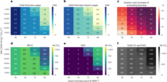
Heat maps of cost-optimal configurations for achieving a net-negative (−110%) emissions target when varying the price of biomass imports (x axis) and DAC capital expenditure (y axis). For comparison between different used metrics in literature: DAC capital costs (CAPEX) of €1,500–7,000 kg⁻¹ CO₂ h⁻¹ correspond to €171–800 t⁻¹ CO₂ per year at a full utilization rate or a capital cost of €16–75 t⁻¹ CO₂ (not including operational expenditure) with a 7% discount rate and a 20-year lifetime. The assumed capital cost of the carbon capture unit for BECC is here assumed at a constant €2,400 kg⁻¹ CO₂ h⁻¹, but it is likely that cost progressions for DAC would spill over also to BECC. a, Total biomass usage. b, Biomass imports. c, The system cost increase of excluding biomass compared to the least-cost solution for all combinations of carbon sequestration capacity and upstream emissions of biomass imports. d–f, BECC (d), DAC (e) and total CC and DAC (f).

Full size image

The system cost of excluding biomass varies between 13–25% (€104–205 billion) at DAC capital costs corresponding to €171–800 t⁻¹ CO₂ per year and a baseline biomass import price of €54 MWh⁻¹. Thus, BECC is substantially more cost competitive even with optimistic DAC investment costs. This is likely to inhibit the scale-up of DAC and therefore its cost progression through technological learning, which is subject to large uncertainties even in the case of gigaton-scale deployment¹⁰⁸ (Extended Data Table 4). To achieve high capacity factors and thereby keep costs down, DAC benefits greatly from a stable and substantial supply of electricity and heat¹⁰⁸, and the energy source can only cause small or zero emissions to enable net-CO₂ removal¹⁰⁹. The absence of these conditions in the short to medium term on a European scale prevents a large scale-up of DAC (and thereby cost progression). In contrast, BECC can be scaled up already in the short term, provided that sufficient biomass is available.

Excluding biomass use in a fossil-free energy system adhering to a negative (−110%) emissions target results in a 20% higher system cost and a substantially larger and more challenging expansion of VRE, electrolysers, electrofuels and DAC compared to if biomass is available. The cost increase is similar to the cost of excluding wind power, and the main reason is the high value of renewable carbon rather than of the energy provision of biomass. It matters less whether biomass is used for combined heat and power, liquid fuel production or industrial process heat, as long as the carbon content is utilized to a high extent, as facilitated through carbon capture to provide renewable carbon for negative emissions or for production of fuels for further use in the energy system. There is large potential for carbon capture also in Fischer–Tropsch biofuel production, where ~70% of the biogenic carbon ends up in the waste stream unless additional hydrogen is added to utilize more of the carbon directly (electrobiofuels). Similar results emerge for a net-zero emissions target, but biomass can then be excluded at a 14% system cost increase due to a lower negative emissions requirement. DAC costs are highly uncertain¹⁰⁸ and substantially affect the system cost of excluding biomass, which explains some of the diversity of results in the literature (Extended Data Table 4), but BECC was found to remain more cost effective even at low DAC costs across a range of assumptions.

A shortage of either carbon-neutral biomass, VRE or hydrogen primarily affects renewable liquid fuel production, which entails the most conversion losses in the energy system and thereby is the marginal emissions abatement option¹¹. Ramping up sufficient resources for liquid fuel production is therefore particularly challenging. Limiting fuel demand through, for instance, electrification and modal shifts would make energy supply to achieve emissions targets easier, whereas developing a portfolio of different fuel supply options appears as a sensible strategy to hedge against the considerable resource and technology uncertainties. Consideration of higher CO₂ sequestration levels would allow for more fossil fuels combined with carbon capture, which would increase the manoeuvring space and decrease the importance of biomass and of any renewable technology but would also rely on a stronger ramp-up of (BE)CCS (Fig. 6d).

In previous studies, biomass use has varied considerably but has often focused on bioelectricity and liquid fuels³⁶, whereas power system studies on firm generation have indicated a value of biomass for handling variability⁸. With a high spatio-temporal resolution and broad cross-sectoral coverage, our study shows that even though substantial dispatchable generation capacities are deployed, they are only rarely used, and thus only a small amount of biomass is allocated for providing flexible bioelectricity. However, although substantial amounts of bioelectricity and CHP appear as low-priority options for biomass usage in this study (similarly to Williams et al.⁷⁸), many near-optimal solutions for biomass usage were found to exist, with similar results for both restrictive and higher carbon sequestration capacities. Thus, small deviations in settings may lead to large differences in biomass usage, and care must be taken when deriving general conclusions.

Given the many near-optimal solutions for biomass usage, local differences in terms of availability of biomass and non-fossil electricity and transmission bottlenecks and carbon infrastructure, the possibility to utilize excess heat in district heating and regional system adequacy considerations lead to local variations in cost-competitiveness of different options (as evidenced already by the diversity of solutions on the country-level resolution, as seen in Extended Data Fig. 6). This probably results in a diversified portfolio of locally optimal biomass usages and spatially resolved trade-offs between using captured carbon for fuel production or for sequestration.

Nevertheless, as also found in previous studies with lower operational resolution^37,39,41, combining biomass usage with carbon capture was found to be a robust strategy. Whereas these earlier studies only include CCS, this study also includes CCU and finds both very valuable to enable high carbon efficiencies in a renewable energy system. Allowing more fossil fuel usage compensated through CDR did not substantially affect near-optimal biomass usage (in contrast to Grant et al.⁴⁸), but it was found to reduce the competitiveness of using captured carbon to produce electrofuels (CCU), in favour of sequestering it (CCS). In fact, failing to apply carbon capture resulted in a considerably reduced value of using biomass in the energy system. Owing to its high investment cost, carbon capture was found to be cost effective in processes running with high utilization rates and not in applications managing the integration of variable renewable electricity.

A net-negative target for the European energy system is probably needed to reach territorial net-zero emissions, considering that residual emissions in other sectors need to be compensated; this might exert a substantial demand pull for biomass, especially if VRE and electrolyser deployment falls behind expectations. The resulting level of biomass usage may even exceed the lower end of estimated global biomass residue potentials, which spans a wide range of 3–21 PWh per year (ref. ¹¹⁰).

Estimated production costs for primary non-residue biomass (for example, Millinger et al.¹¹¹) fall within competitive cost ranges in this study, especially if biomass residues are limited. Thus, high biomass demand and prices could provide an incentive for the forest and agriculture sectors to produce more primary non-residue biomass for the energy system. The land carbon consequences in such a scenario are uncertain; studies find that biomass demand can induce changes in land use affecting land carbon stocks positively or negatively, depending on climate and soil conditions, historic land use, character of biomass production system being established, governance and other geographically varying factors^{104,112,113,114,115,116}.

The technical BECCS potential associated with domestic biomass residues in Europe (excluding forest residues) has been estimated at 200 Mt CO₂ (ref. ¹¹⁷), which would not suffice to achieve net-negative emissions targets. For the new EU Renewable Energy Directive III, energetic usage of primary forest residues was proposed to be excluded as an option for meeting renewable targets¹¹⁸, which alone have been estimated to amount to up to 1.6 PWh per year in Europe⁸³, or up to 600 Mt biogenic CO₂ that could potentially be captured (Extended Data Table 2). Excluding comparably easy-to-monitor domestic resources might lead to a substantially higher cost of the energy system and to a higher demand for imported biomass and dedicated crops, with harder-to-foresee environmental consequences. As has been shown here, biomass usage, combined with carbon capture, is cost effective as long as net upstream emissions are relatively small or if negative emissions counteract limited upstream emissions. Exclusions of biomass sources such as primary forest residues thus need to be weighed against the targets in the energy sector and the potential to achieve negative emissions and gauged towards achieved capacity expansion speeds for VRE and electrolysis, which require an unprecedented ramp-up to achieve the results presented here already if biomass is not restricted.

PyPSA-Eur-Sec model

PyPSA-Eur-Sec^60,119 is an open-source, sector-coupled full European energy system optimization (linear programming) model including the power sector, transport (including also international shipping and aviation), space and water heating, industry and industrial feedstocks. The model minimizes total system costs by co-optimizing capacity expansion and operation of all energy generation and conversion and of storage and transmission of electricity, hydrogen and gas. The model is based on the Python software toolbox PyPSA (Python for Power Systems Analysis)¹²⁰. A comprehensive description of the model can be found in Neumann et al.¹²¹. A version with an extended set of biomass resource technology portfolio is used¹¹, with added details for carbon capture energy penalties and additional competition introduced for industry heat supply and added domestic biomass pellet boilers, hydrogen CHPs, waste incineration and electrobiofuels (biofuels with extra hydrogen added to the process to utilize more of the biomass carbon directly).

A 37-node spatial resolution and a 5-h temporal resolution over a full year in overnight greenfield scenarios was used, based on a trade-off between the difference in results compared to with a 1-h resolution (Supplementary Fig. 1) and computing time (Supplementary Fig. 2). A country-level spatial resolution was chosen for computational reasons. A lossy transport model for electricity transmission was used, which is suitable at this resolution¹²², and transmission is constrained to expand to at most double the total line volume in 2022.

Final energy demands for the different sectors are calculated based on the JRC IDEES database¹²³ with additions for non-EU countries (refs. ^10,60 provide further elaboration) and need to be met (that is, demand is perfectly inelastic). However, energy carrier production including electricity, hydrogen, methane and liquid fuels is determined endogenously. Fossil fuels (coal, natural gas and oil) and uranium are included, as are solid biomass imports as outlined below. Technology costs and efficiencies are elaborated on in the Supplementary Information, with technology values for 2040 (given in €₂₀₁₅) used from the PyPSA energy system technology data set v0.6.0 (ref. ¹²⁴). The discount rate is uniform across countries and set to 7%, except for rooftop solar PV and decentral space/water heating technologies, for which it is set to 4%.

Mathematical formulation

The objective is to minimize the total annual energy system costs of the energy system that comprises both investment costs and operational expenditures of generation, storage, transmission and conversion infrastructure. To express both as annual costs, we use the annuity factor (1 − (1 + τ)⁻ⁿ) / τ that converts the upfront overnight investment of an asset to annual payments considering its lifetime n and cost of capital τ. Thus, the objective includes on one hand the annualized capital costs c_* for investments at bus i in generator capacity G_i,r ∈ R⁺ of technology r, storage energy capacity E_i,s ∈ R⁺ of technology s, electricity transmission line capacities P_ℓ ∈ R⁺ and energy conversion and transport capacities F_k ∈ R⁺ (links) and the variable operating costs o_* for generator dispatch g_i,r,t ∈ R⁺ and link dispatch f_k,t ∈ R⁺ on the other:

Thereby, the representative time snapshots t are weighted by the time span w_t such that their total duration adds up to one year; ∑_t∈Tw_t = 365 × 24 h = 8,760 h. A bus i represents both a regional scope and an energy carrier. In addition to the cost-minimizing objective function, as exhaustively described in ref. ¹²⁵, we further impose a set of linear constraints that define limits on the capacities of generation, storage, conversion and transmission infrastructure from geographical and technical potentials and the availability of variable renewable energy sources for each location and point in time. Further, the limit for CO₂ emissions or transmission expansion is defined, along with storage consistency equations, and a multi-period linearized optimal power flow formulation. Overall, this results in a large linear problem.

The modelled system represents a long-term equilibrium where the zero-profit rule applies and the revenue that each generator receives from the market exactly covers their costs^126,127. By way of annualization of capital costs (assuming that the modelled year represents an average revenue year for each asset over their economical lifetime) and weighting of asset operation to the interannual temporal resolution, there is therefore full cost recovery of all assets built. Prices form endogenously in the model based on renewable supply conditions, storage and demand flexibility. Regional electricity price time series are retrieved from the dual value of the energy balance equations for each region and hour. CO₂ emissions are considered in the model, whereas other GHG emissions are not, and a CO₂ price is calculated as the shadow price of the least-cost objective function for achieving the set emissions target.

Near-optimal analysis

The Modelling to Generate Alternatives (MGA) method^{70,72,73,74,128} was implemented for the sector-coupled model. With this method, first a cost-optimal result for achieving emissions targets is calculated, which gives a minimum system cost C. For notational brevity, let c^Tx denote the linear objective function equation (1) and Ax ≤ b the set of additional linear constraints in a space of continuous variables, such that the minimized system cost can be represented by

In the next step, this cost is increased by ε ∈ {0.01, 0.02, . . .} and set as a constraint, while minimizing or maximizing a set of variables, such as energy carriers or technologies, for example, total biomass usage, total biofuel production or total wind power generation, with

By exploring the extremes, the Pareto frontiers for a given parameter–cost combination are mapped out. The system cost of excluding a particular technology or resource was validated in runs where the option in question was excluded. To obtain shadow prices related to system cost for Fig. 5, biomass use was set as an additional constraint in cost-minimizing runs.

The model runs were performed on the Chalmers Centre for Computational Science and Engineering (C3SE) computing cluster.

Biomass and bioenergy

A variety of biomass categories and conversion technologies are introduced in the model. Different biomass residue types are clustered into the categories solid biomass and digestible biomass (Extended Data Fig. 4). Solid biomass can be used for a variety of applications in heat, power and fuel production and can optionally be combined with carbon capture (Extended Data Fig. 1). Digestible biomass can be used for biogas production via anaerobic digestion, which is upgraded to pure biomethane with the option to capture the waste CO₂ stream. Methane can also be produced via gasification of solid biomass (BioSNG), or supplied by fossil methane. These routes result in the same end product, methane (CH₄).

Medium domestic (country-level) biomass residue potentials for 2050 from the JRC ENSPRESO database were used⁸³ nodally explicitly, with a weighted average of country-level biomass costs including harvesting, collection and transport from the reference biomass scenario¹²⁹. Additionally, more expensive solid biomass imports can be used¹¹ (Extended Data Fig. 3 and Extended Data Table 2). Pre-treatment of biomass, where needed, is considered implicitly through moderate conversion efficiencies and spare waste heat that could be utilized. Small-scale heating includes a pelletization cost of €9 MWh⁻¹ biomass. Reflecting current EU policy direction, bioenergy feedstock is assumed to consist of residues, for which the likelihood of direct and indirect land-use change and land carbon changes is smaller than for dedicated feedstock production. The use of residues and waste as bioenergy feedstock is assumed not to influence the land carbon stock; that is, the global net flow of CO₂ between the atmosphere and the biosphere, which is driven by photosynthesis, respiration, decay and combustion of organic matter, is assumed to not be affected. In a renewable energy system, processing, conversion and transport do not cause fossil carbon emissions, and residual GHG emissions associated with land use can be considered to be offset through CDR if exporting countries adhere to net-zero or net-negative targets.

For biomass imports, as described in ref. ¹¹, we assume that 175 EJ per year of biomass can be supplied globally at a price of US$15 GJ⁻¹, using the average of an IAM comparison⁵⁴. Using regional data on biomass use per capita and population estimates¹³⁰, we assume that up to 20 EJ biomass (subtracting domestic potentials) may be imported to Europe at a price of €15 GJ⁻¹ (€54 MWh⁻¹). For each additional EJ to be imported, the price is assumed to increase by €0.25 GJ⁻¹, based on the slope of the low-cost scenarios (Extended Data Fig. 3). The assumed import prices are substantially higher than 2020 wood chip prices at €20–25 MWh⁻¹ (ref. ⁸⁹) (Extended Data Fig. 3). This reflects an increased demand for biomass in scenarios complying with stringent GHG emission targets. We test the effect of this assumption on results in a sensitivity analysis (Fig. 7). Direct biofuel imports (and hydrogen derivatives) from outside Europe are not considered.

Carbon balances of biomass

Solid biomass carbon dioxide uptake from atmosphere, with a carbon share %C_sb= 50%, specific energy e_sb= 18 GJ t⁻¹ and molality ({{rm{m}}}_{mathrm{C{O}_{2}}}/{{rm{m}}}_{C}) = 44/12 (equation (5)):

Liquid fuel carbon dioxide emissions (t CO₂ MWh⁻¹) at full combustion for diesel and methane based on -CH₂– simplification and specific energy ({e}_mathrm{C{H}_{2}}) = 44 GJ t⁻¹ LHV for diesel and ({e}_mathrm{C{H}_{4}}) = 50 GJ t⁻¹ LHV for methane (equation (6)):

The carbon efficiency η_c of the conversion is estimated by equation (7).

The rest is assumed to end up as CO₂, of which a part ε_s is separated and possibly captured with an efficiency η_ε, with the remainder ε_v being vented as CO₂ to the atmosphere in the exhaust gas.

The biogas produced from digestible biomass is assumed to contain 60 vol% CH₄ (specific energy e = 50 GJ t⁻¹, density ρ = 0.657 kg m_n⁻³) and 40 vol% CO₂ (ρ = 1.98 kg m_n⁻³), which calculates to 0.0868 t CO₂ ({mathrm{MWh}}_{{mathrm{CH}}_{4}}^{,,,-1}). The feedstock input potentials and costs for biogas are given for MWh({mathrm{MWh}}_{{mathrm{CH}}_{4}}) and thus MWh_in= MWh_out for the carbon balance calculations. Thereby the C content in the slush can be omitted, thus avoiding system boundary issues with the agricultural sector.

Carbon capture

Process emissions are assumed to be captured post-combustion through solvents, which is the standard method with highest technological readiness level in 2021¹³¹. For carbon capture in biomass applications, part of the biomass input is used to meet the additional heat demand for regenerating the solvents used for CO₂ capture. Heat is assumed to be met by a steam boiler of the type suitable for the process (gas for biogas, otherwise solid biomass), with capital and operational costs added accordingly. Capture rates of 95% are assumed for these processes except for biogas, where 90% is assumed. For biofuel production, acid gas removal (including CO₂, amounting to 71% of the carbon in the biomass feedstock; Supplementary Table 1) from the syngas is assumed to be performed with the Rectisol¹³² (methanol-based) process, with a 90% capture rate^133,134,135 and electricity demand to cover for this is assumed to be included in the base process. The effect of capture rates (which can be both higher and lower than assumed here) is assessed in a sensitivity analysis (Extended Data Fig. 5). As a result of energy penalties of the BECC processes, the efficiency of the conversion to the main product is decreased, and the capital cost is increased to cover for the additional heat demand and carbon capture infrastructure, as summarized in Extended Data Table 1. In contrast, heat demand for DAC can be met by several competing process steam options as described below.

A scaling factor α for the additional biomass needed to supply the steam heat demand of carbon capture is calculated as a function (equation (8)) of the amount of CO₂ in the output stream ε_s (Supplementary Table 2), the required heat input for carbon capture e_th,cc (here assumed as 0.66 MWh t⁻¹ CO₂ at 100 °C (ref. ¹³⁶)) and the boiler efficiency η_th (Supplementary Table 2).

The steam efficiency η_steam (equation (9)) and main product efficiency η_new (equation (10)) are derived as a function of the scaling factor α.

The new investment cost C_I,new is derived as a function (equation (11)) of the investment cost of the base plant configuration C_I,old scaled by the updated efficiency η_old/ η_new, with added investment costs for the steam boiler C_I,th scaled by the steam produced η_steam/ η_new and additional investment costs for the carbon capture unit C_I,cc (here assumed as €2,400 kg⁻¹ CO₂ h⁻¹ (ref. ¹³⁶)) scaled by the process CO₂ output stream ε_s.

For CHP units, the heat demand is scaled as the main product, with added district heat output from the carbon capture process (here assumed as 0.79 MWh_tht⁻¹ CO₂ at district heat temperature¹³⁶).

These calculations result in the costs and efficiencies for the processes with carbon capture shown in Extended Data Table 1.

Sector-specific assumptions

Steel production is assumed to be fully performed with hydrogen as a reduction agent (direct reduced iron, DRI) and electric arc furnaces, and the share of scrap steel increases from 40% in 2023 to 70% in the target year. Cement production entails unavoidable emissions from calcination, which can be captured.

District heating is assumed to cover 30% of urban demand, whereas space heating demand is assumed to decrease by 29% due to efficiency gains through new buildings and building renovation. District heat can be fulfilled by numerous options, including excess heat from electrolysers and fuel production (of which 50% is assumed possible to use considering that processes are not always near district heat grids) and mandatory incineration of municipal solid waste.

Industrial heat is divided into three segments: low (process steam, <200 °C), medium (~200–500 °C) and high temperature (>500 °C). In the low- and medium-temperature segments, biomass is an option, whereas methane and hydrogen are an option in all three. Direct electrification is an option in the low-temperature (process steam) segment, whereas heat pumps for process steam are not considered. Thus, solid biomass competes for producing industrial process steam with electric, hydrogen and methane boilers and for producing medium-temperature process heat with hydrogen and methane.

Base electricity demand for households and industry is the same as in 2011 (except for a subtraction of electricity used for heating, the supply of which is endogenously determined), with a temporal variation as depicted in Fig. 3.

It is assumed that a strong increase in the use of electric vehicles reduces liquid fuel demand in land transport to zero, hence reducing the need for biomass and/or electricity for meeting renewable fuel targets (land transport demand overall is assumed to increase by 20%). A liquid fuel demand is however retained in aviation (total fuel demand increases by 70% compared to 2011), shipping (+50% compared to 2011, with half of the fuel demand supplied by hydrogen) and in the chemical industry (same demand as 2011), which can be supplied through solid biomass-based liquid fuels (biofuels), electrofuels, electrobiofuels and fossil fuels. Transport and chemical demand is assumed as for the year 2060 in Millinger et al.¹¹, and recycling of plastics is not considered.

For a sensitivity analysis with less sector coupling, the following options were turned off completely: battery electric vehicle (BEV) charging demand-side management; vehicle to grid; thermal energy storage; waste heat usage from biofuels, electrolysis, DAC and BioSNG; H₂ networks; H₂ underground storage in salt caverns. Further, no expansion of the electricity transmission or district heat grids from 2022 levels was allowed.

Cost estimations

Costs of energy provision to different applications are estimated as follows and used for comparing cost increases to sectoral costs. The cost of, for instance, fuels is estimated by allocating the cost of feedstocks used by the share of total feedstocks used for fuel production and adding investments and operational costs. For processes with several outputs, the Carnot method is used for allocating costs to different products³⁴.

Assuming 60 °C for heat output and 20 °C for the sink, a Carnot factor for heat is derived by equation (12)³⁴:

The allocation factor a_th is derived by considering conversion efficiencies for all products (equation (13)): heat η_th, electricity η_el, fuels η_fu and multiplying them with their Carnot factors. Carnot factors for electricity, hydrogen and fuels are set to one.

The share of H₂ used for electrofuel production is calculated by dividing the electrofuel H₂ demand ({delta }_{i,,j,t}^{,{mathrm{H}}_{2}}) for all electrofuel technologies j ∈ F_e, by the total H₂ production ({pi }_{i,t}^{,{mathrm{H}}_{2}}). The cost of H₂ (including electricity, electrolyser capital costs and H₂ pipeline costs ({C}_{jinmathrm{H}_{2}})) is assigned to electrofuels by the share of H₂ used for electrofuel production. The total cost is calculated as in equation (14).

The cost of solid biomass b_s used to produce biofuels is assigned to the biofuels by the amount of solid biomass used for biofuels ({delta }_{jin {F}_{mathrm{b}},i,t}^{,{b}_{mathrm{s}}}), with j ∈ F_b divided by the total amount of solid biomass used ({pi }_{i,t}^{,{b}_{mathrm{s}}}). This is added to the capital cost of biomass to liquid ({C}_{i}^{,{F}_{mathrm{b}}}) (equation (15)). The cost is allocated to fuels and heat by equation (13).

Costs for industry heat are straightforward, as there is only one product, and they are calculated as above.

Technology growth rates

Historical technology growth rates are used to ex-post assess feasibility of future growth expectations and model results¹³⁷, but not to restrict model results. Technology growth typically follows an S curve and is often estimated by a Gompertz curve. The maximum growth rate G_gmp at the inflection point of the S curve serves as an indicator for comparison to historically observed growth rates and is calculated by equation (16)⁹⁰.

where L is the asymptote (set to the obtained cost-optimal result for individual technologies), k is the growth constant and e is Euler’s number.

Δt is the time (in years) it takes to grow from 10 to 90% of the asymptote and can be estimated by equation (17)⁹⁰.

Setting the growth constant to k = 0.09 gives Δt_gmp= 34 years (equation (17)), that is, if starting at 10% in 2023, 90% of the asymptote is achieved in year 2057. This setting is used for estimation here.

G_gmp is normalized to the electricity demand at the inflection point, located at 37% of the asymptote L. Demand in the base year δ₀= 3,448 TWh (ref. ⁸⁴) and demand δ_T in the target year is set to the resulting electricity generation of the respective scenario.

Limitations

A limitation compared to IAM studies is the lack of an explicit representation of agriculture and forestry, and the lack of a global trade model (including economy dynamics and equilibrium modelling). An expansion of the system boundaries to encompass the land-use system would more accurately capture emissions flows related to biomass and capture the competition between BECCUS and land-based CDR measures such as Afforestation/reforestation²³. Afforestation/reforestation has a substantial CDR potential²⁴, but there are uncertainties regarding permanency and additionality compared to geological sequestration²³. Combined with other CDR measures such as enhanced weathering, biochar and direct ocean capture²⁴, the necessity of achieving negative emissions in the energy sector and thus the role of biomass may be reduced.

A chemical demand is included, but demand may deviate from the assumed levels, and other uses such as construction and biochar may also compete for biomass residues (which stem from forestry, from which the main product is mainly used for construction), which is not considered in this work.

A spatially explicit representation of geological carbon sequestration locations and of infrastructure for CO₂ transport was not considered and should be pursued in further work. Similarly, whereas a constant cost for biomass transport to where it is used is contained in the biomass residue cost, the specific transport distance required is not assessed. Whereas the overall results are not notably affected by assumptions on biomass residue and carbon handling costs, the practical spatial implementation probably is. Further work should assess spatial aspects of carbon and biomass management^138,139 and connected logistics challenges¹⁴⁰. For computational reasons, a spatially more explicit assessment could not be performed with the diverse biomass technology portfolio and competitions across all sectors we consider in this study, and for the same reason, a weighted average of domestic biomass residue costs was used.

Leakage of methane and hydrogen is not considered and presents a risk when relying on gaseous fuels¹⁴¹. However, digestible biomass combustion may avoid methane emissions, which would otherwise occur, which is valuable in its own right but not considered within the system boundaries given here.

In runs with higher carbon sequestration, more fossil fuels are used, which affects emissions of logistics of, for instance, biomass, which is not considered as it would render the optimization problem non-convex and substantially more computationally intensive. Upstream emissions of fossil fuels are also not considered, which would affect results at higher carbon sequestration capacities.

Land transport was exogenously assumed to be fully electrified, whereas electric or hydrogen-fuelled aviation was not considered as a conservative assumption based on expected long lead times delaying a substantial market penetration. Assumptions on fuel demand levels in these sectors influence results by affecting primary energy demand and costs more than any other part of the energy system¹¹.

For the weather data we use historical data from 2013, which is regarded as a characteristic year for wind and solar resources¹²¹. Interannual weather variability has an impact on variation management and firm generation but is not assessed here. Whereas firm dispatchable capacities can cover for almost the whole inflexible demand already in the results given here, both more and less biomass would be used for that purpose in more extreme years, and the assessed case may be seen to represent an average biomass usage case. The model was run with perfect foresight of weather conditions and demands, whereas in reality, there is substantial uncertainty in capacity planning and adequacy requirements. This is especially important for combined capacity and dispatch optimization as performed here and affects results on firm generation requirements. However, substantial firm capacity is deployed in the results but very seldom run. Given the low biomass amounts, even a doubling would not affect results substantially. Also, whereas flexibility is assumed in electrolysers, BEVs and so on, there is a part of the electricity demand that is assumed not to be flexible, where some flexibility (demand elasticity) could be assumed and which would reduce the need for firm generation. Future work should assess these aspects and demand variations (flexibility and absolute amounts) further.

A greenfield assessment was performed, which does not take existing infrastructure into account, aside from existing power transmission lines and hydropower installations. Emphasis in this work is to assess the diversity of system compositions of an energy system adhering to stringent emissions targets, not on the transition leading there. The timing of when net-zero or net-negative targets in the energy system are achieved is uncertain, and the results here are not tied to a specific year. If targets are achieved by 2050 or later, most current capacity would have reached the end of their lifespan. In the event that targets would be achieved as early as 2040, some energy infrastructure existing in 2024 is likely to remain, but these capacities amount to a small fraction compared to the capacity expansion seen in the results. Nuclear capacity that began operation after 1990, or is currently under construction, amounts to 29 GW (ref. ¹⁴²), able to produce 2% of the total electricity generation in the least-cost net-negative scenario. For dispatchable gas generators, 242 GW_el capacity was in place in the region in 2022¹⁴³, or 46% of the gas power capacity obtained in the least-cost net-negative scenario. Thus, accounting for any remaining gas power capacity in the target year would not affect results. Therefore, we deem this to be a mild limitation to the modelling.

We acknowledge the limitation of this study in focusing solely on the solution space concerning the composition of a system adhering to very stringent emissions targets, rather than analysing the transition towards achieving these targets over time. Conducting a detailed analysis of the energy transition over the years would require a reduction in spatial and temporal resolution to ensure computational feasibility, leading to the loss of detail on other valuable aspects of the analysis. Nevertheless, we recognize the importance of further research to analyse the transition dynamics in achieving emissions targets over time, considering both short-term variability and long-term capacity planning.