Drivers of mesoscale convective aggregation and spatial humidity variability in the tropical western Pacific

Introduction
Water vapour, as the principle greenhouse gas, is a major determinant of the tropical energy budget. Future changes of water vapour constitute a positive feedback in climate models, which predict an increase in specific humidity approximately consistent with a zero-order assumption of constant relative humidity1. However, spatial changes in water vapour may modify this basic response, which in the tropics are associated with the spatial arrangement of convection in a two-way interaction. The likelihood of deep convection and associated convective precipitation increases exponentially with total column water vapour (TCWV)2,3,4. The local aftermath of convection is a near saturated free troposphere due to the detrainment of saturated, cloudy air. The net drying of the troposphere due to precipitation is manifested in areas remote from convection associated with subsidence5. Deep convective activity in the tropics migrates around the interior and especially boundaries of a moist region with column-integrated humidity exceeding 48 kg m−2, separated from the dry subsidence regions by sharp horizontal moisture gradients6. Knowledge of this allowed simple models to be constructed that could grossly reproduce the tropics-scale distribution of water vapour based on column saturation over the highest sea-surface temperatures (SSTs) or regions of upward motions balanced by advection and compensating subsidence elsewhere7,8. These models, thus, help us to explain the climatological relationship between TCWV and SST9.
While these broad, tropics-scale models can explain the mean climatology of the water vapour distribution and radiation budget, there is recent evidence that the details of the arrangement of convective clouds, or rather its degree of spatial “clustering”, over scales of a few hundred kilometers (the beta and alpha mesoscale) also matter if temporal variations in the tropical energy budget are to be understood. When combined with low level static stability that determines low cloud amount, the deep convective arrangement (as measured by a metric Iorg10), has been demonstrated to explain much of the variability in the net tropical radiation budget over monthly to annual time-scales11. This is a particularly intriguing result, since Iorg measures convective clustering almost exclusively on the beta mesoscale (20-200km)11,12. Thus, mesoscale variations in the arrangement of convection appear to not only determine the moisture budget directly in deep convective regions on the mesoscale itself, but also consequently impact the humidity reaching the drier “radiator fins”13 and, in turn, determine the energy budget of the wider tropical atmosphere according11. Understanding what determines the mesoscale organisation of convection and associated patterns of mesoscale humidity variability is, therefore, crucial for gaining insight into the drivers of variations in the wider tropical radiative budget. This may also be important for assessing tropical climate sensitivity.
Further motivation is provided by previous idealized simulations of radiative-convective equilibrium with cloud-resolving models, which show that increased convection clustering leads to drier mean atmospheres14,15,16,17. In support of this, an association was found between the degree of organisation of convection in the tropical Atlantic and the spatial variance of column water vapour18. Thus, if convective aggregation changes in a warming climate, it could alter tropical climate sensitivity19. Unfortunately, initial attempts to assess this using model inter-comparisons have failed to show consensus20.
One hindrance to progress is the difficulty of assessing mesoscale convective organisation with presently available observations. In a recent review by Biagioli and Tompkins12, metrics of convective organisation were divided into direct and indirect categories. Direct measures of organisation attempt to identify the location of convective updrafts which must be presently achieved using retrievals of cloud-related properties or precipitation. While such observations can reveal larger-scale organisation of convectively-coupled waves, such as the Madden Julian Oscillation21, eastward propagating moist-Kelvin waves, and westward propagating Rossby waves for example22,23,24,25,26, cloud overlap complicates the identification of the arrangement of convective elements over the beta-mesoscale27,28 despite the application of filters to try to mitigate such effects and identify overshooting tops11.
In contrast, indirect metrics try to identify the impacts of convective clustering, with increased clustering associated with larger spatial variance in column-integrated humidity or moist static energy (MSE)29. One limitation of such univariate signatures is that they are sensitive to other factors, such as mean lower boundary temperature. For example, column-mean MSE increases with a warmer surface temperature and, thus, MSE variance would also be expected to increase in tandem. However, cloud-resolving model studies have also documented the impact of convective clustering on the multivariate relationships between SST, water vapour variance, clouds, and precipitation30. To date, limited analogous use of such multivariate metrics has been applied to observations to gauge the impact of mesoscale organisation.
Here, we aim to further understand the mesoscale controls of tropical humidity variability, its association with deep convective organisation, and its impact on the local radiative budget in state-of-the-art observations of the tropical western Pacific available from October 2016 to December 2019. We apply a simple multivariate analysis technique adopted from idealized modeling studies to Pacific warm pool regions of a similar size to the domains used in numerous numerical studies of convective aggregation that are subject for parts of the year to spatially homogeneous lower boundary conditions, also reminiscent of the idealized studies. We use this “natural laboratory” to show how humidity variability changes throughout the year and how tropical wave activity acts to mix up and homogenize water vapour in distinct episodes that impact the local energy balance.
Results
Mean seasonal climate
The organisation of convection is assessed using a multivariate analysis of atmospheric retrievals of TCWV, SST, cloud, and rainfall for mesoscale sized regions of approximately 106 km2 in the tropical western Pacific (Fig. 1), a size typical of the domains used for idealized studies of convective aggregation (see methods). The key focus region analysed lies to the north of the equator from 2°N to 9°N and from 135°E to 145°E. This region was chosen as it lies in the western Pacific warm pool region, is distant enough to avoid direct influences from the maritime continent, is subject to a seasonal evolution of SST gradients, and is close to the regions studied by Tobin et al.28,31. For robustness, we also analyse two other mesoscale-sized regions: one further east between 3°N to 10°N and 147°E to 157°E and one straddling the equator between 3°S and 4°N and 156°E and 166°E. Additional analysis of these secondary regions is contained in the supplementary material.

The SST contours start from 301.75 K and increase every 0.25 K. The rectangles delimit the three study regions, with the dashed lines denoting the main area focused on, with the other two secondary regions used to test the robustness of the conclusions.
In terms of the annual cycle, the SST in the focus region is subject to a weak meridional gradient of around 1 K across the 7 degrees of latitude during the boreal winter/spring when the main warm pool migrates south of the equator and the southern Pacific convergence zone strengthens, while mean SST gradients are virtually absent in the summer/autumn months (Fig. 2). The maximum rainfall occurs in the summer (JJA) months, reducing somewhat in magnitude during the boreal autumn period, as expected from the well known seasonal migration of the inter-tropical convergence zone (ITCZ). In contrast, during the summer and autumn months, precipitation is meridionally homogeneous across this domain, consistent with the homogeneous SST.

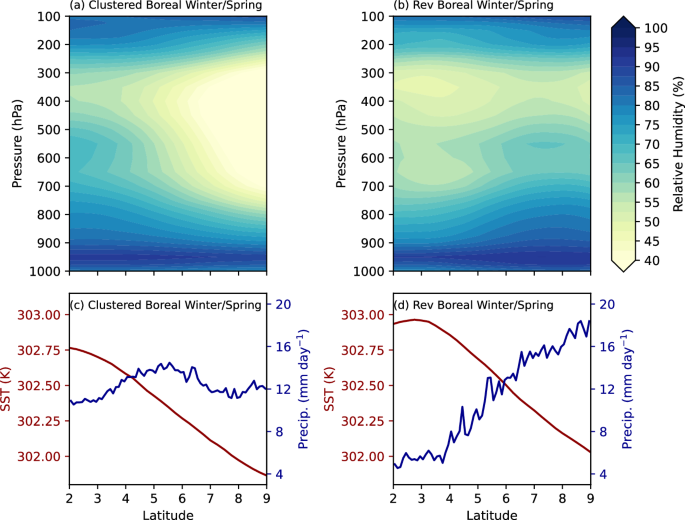
a–d Seasonal mean variations of ERA5 relative humidity as a function of latitude and height (left panel), and domain-mean relative humidity as function of height (right panel, see legend). e–h The seasonal mean Himawari SST (red, left axis) and GPM IMERG rainfall (blue, right y-axis) as a function of latitude.
As the SST cools by around 1 K during the boreal winter, with the main warm pool migrating south of the equator, the rainfall also reduces, with a local peak at 6°N. This meridional gradient of precipitation is most pronounced in spring (MAM), with mean rainfall changing by more than a factor of two, while the main precipitation maximum lies to the south of the equator in the southern Pacific convergence zone, outside the domain of focus. The tropical winds show shifts in the circulation (Fig. S1), with the summer and autumn marked as a low mean wind regime, and near-surface winds less than 4 m s−1, which increases to over 6 m s −1 at 700 hPa. Thus, the lower tropospheric wind-shear of the wind magnitude, while weak, is still larger than the winter/spring months, where the boundary layer zonal winds are stronger but lower tropospheric shear is almost absent. This has potential implications for aggregation since weak tropospheric shear is not adequate to form convection into mesoscale squall lines32,33 and can prevent clustering through the homogenization of water vapour structures34. Modeling work has shown that precipitation decreases from no shear to weak shear due to the inhibition of aggregation, but then increasing as stronger shear leads to mesoscale convective system formation35,36. Recent observational work has again emphasized the potential importance of wind shear for convective aggregation37.
These shifts in the convection distribution and wind-shear are major determinants of the spatial variability of water vapour. The mean meridional gradient from June to November is very limited throughout the troposphere, consistent with the uniform distribution in rainfall and indicative of randomly distributed deep convection. This contrasts with the situation in the boreal winter and spring months, where there is a north-south gradient of relative humidity above the boundary layer, with mean mid-tropospheric relative humidity as low as 40% in the northern part of the domain. In summary, the spatial variability of water vapour is minimum in the JJA-SON months and at a maximum in the DJF-MAM months. While large-scale ocean dynamics set up the north-south gradient of convection in winter/spring, we will see in the energy balance (Impacts of reversal events) calculation that the radiation budgets tend to amplify this.
A multivariate analysis of water vapour, SST, and precipitation co-variability
The evolution of the sub-seasonal variability of water vapour and its relation to convection and SST is examined using a simple multivariate analysis (see methods), which is interpreted in terms of previous idealized modeling of convection using high resolution, convective permitting models coupled to simplistic slab ocean models38. While a fixed-depth, slab ocean neglects the intricacies of ocean dynamics, it can shed some light on simple ocean-atmosphere interaction. The cloud resolving model was integrated for many weeks, starting from homogeneous initial conditions where deep convection was initially randomly distributed through the domain, which after several weeks, evolved to a state in which convection was highly clustered and the majority of the domain was convection free and very dry. In the original analysis of Tompkins and Semie38, the multivariate evolution of the model state was examined using a Hovmöller analysis, ordering the model columns (SST anomalies) according to TCWV (see their supplementary Fig. S4), which we summarize here by taking a multi-day average over two periods covering the initial random phase, and a late clustered phase (Fig. 3a).

a A random and a clustered/aggregated state from results of the slab ocean model of Tompkins and Semie38, with its respective linear fit. b Boreal summer/autumn and winter/spring “reversals” and clustered regimes, using Himawari and MIMIC datasets, with its respective linear fit. In each boxplot, the lower end represents the 25th percentile, the upper end shows the 75th percentile, and the middle line indicates the median (50th percentile). Only the bins with more than 1% of the data are shown. The whiskers extend to the 10th and 90th percentiles. The white square inside the box represent the mean.
In the initial random phase, SST perturbations have limited time to amplify since warming due to clear sky-enhanced SW flux is not sustained for long before a nearby deep convective event occurs, causing anvil shielding and subsequent cooling. Thus, the spatial SST variance is restricted in this phase, and the ubiquitous sources of convective moistening means TCWV exceeds 45 kg m−2 everywhere in the domain (Fig. 3a). In this random phase, enhanced shortwave fluxes at the surface in clear sky regions means SST and TCWV are anti-correlated, and the SST-TCWV regression coefficient (γ hereafter) is negative. This changes once the convection is strongly clustered, with enhanced OLR in the dry regions reversing the SST-TCWV relationship, which is now positively correlated (γ > 0) for most of the range of TCWV values, with the relationship remaining negative only for the moist convective part of the domain with TCWV > 50 kg m−2 probably due to the presence of cold pools38. In this highly clustered regime, both SST and TCWV variance are larger. In the following discussion we will use these relationships as a context for the analysis of convection and water vapour distributions observed in the focus warm pool domain.
Using the same Hovmöller analysis of Wing et al.17 and Tompkins and Semie38, we examine two illustrative periods, one in boreal summer and one in spring, as these represent the extremes in terms of the background humidity gradients. In the boreal summer, when the region of focus lies directly in the main warm pool region, it is confirmed that mesoscale SST gradients are very limited even over shorter time periods (Fig. 4a-d). Temporal changes in the distribution of column water vapour are scant, with the driest 1st percentile of TCWV hovering around, but very rarely breaching the 48 kg m−2 threshold that demarks the boundary between deep convective and non-convective regions in the deep tropics in the present climate6. At this time of year, the driest regions are sometimes found over the SST warm perturbations within the domain (e.g. see episodes around 14th and 23rd July and 11th August), but this is not always so and in any case, the magnitude of the SST anomalies are limited, similar to the pre-aggregation onset random convection phase in CRM experiments38,39. Convection is always associated with the moistest columns, as expected from previous analyses (black contours, panel b)4,40,41. In general, the periods with largest mean rainfall (panel d) are associated with greater lower tropospheric wind shear and largest maximum humidity values within the domain. This situation of a limited TCWV and SST spatial variability, high minimum TCWV values, and anti-correlation between SST and TCWV is reminiscent of random convection in idealized CRM experiments, where convection occurs throughout the domain, providing local moisture sources to prevent the free-troposphere in any region of the domain from substantially drying out (Fig. 3a).

a, e Hovmöller plot of SST anomaly (colours) as a function of absolute TCWV clipped between at the 1st and 99th to remove anomalous extremes, with contours showing percentile values (legend). b, f Hovmöller plot of SST anomaly (colours) as a function of TCWV retrieval percentile, with black contours showing areas of precipitation of 2 mm hr−1. c, g Time-series of the SST-TCWV best-fit linear regression coefficient γ, where SST = γTCWV + C, and the 24-hour running mean γ. d, h Domain mean precipitation rate and vector magnitude wind shear calculated as a difference between the 700 and 1000 hPa levels of ERA5 reanalysis. Green blocks in panels e-h mark reversal events, in which the SST-TCWV regression reverses from positive to negative and remains below one standard deviation for a period of at least 24 hours in the boreal winter/spring. An example boreal summer/autumn (a–d) and winter/spring (e–h) period are represented in the figure.
This situation changes remarkably in the boreal winter/spring, and we show an example of this during April/May 2017 (Fig. 4e-h). In this example, there are two very distinct regimes apparent. Mostly, the humidity variance is much larger than during the summer, with the driest part of the domain reaching values below 30 kg m−2. In this regime, the relationship with SST shows that the coldest SSTs are found at the locations of the driest columns, while as before, the convection and rainfall are still associated with the moistest locations. SST variance is also considerably larger. In contrast to the summer example, this pattern of larger SST and TCWV variance and a positive correlation between the two fields resembles a situation of aggregated deep convection, where convection is restricted to one part of the domain and the minimum TCWV is much drier than the threshold associated with convective activity.
Although this aggregated-like state is the usual situation in the spring period shown, two multi-day “events” disrupt this situation starting around the 12th and 22nd April, respectively. During these events the humidity distributions change substantially. The spatial humidity variability reduces, quite rapidly in the first of the two cases, which is associated with a moistening of the driest regions in the domain by at least 20 kg m−2. The moistest regions associated with convection do not change, as expected since these values are consistent with an approximately saturated moist adiabat. At the same time, the SST-TCWV (γ) relationship reverses (panel f), with the warmest SSTs found together with the driest columns of the domain. These events will thus be referred to as winter/spring “reversals” and, in this example, last for several days before the relationship reverts to the standard winter pattern. As SST evolves slowly, these changes in the SST-TCWV relationship reflect a redistribution of the convective moisture sources relative to the SST patterns, which we will investigate further. We also note that panel h does not appear to reveal a strong association of domain mean precipitation or lower-tropospheric wind shear with these two example reversal events.
Our analysis of Hovmöller plots for other months suggests that convection in this particular region is randomly distributed from June to November when SST gradients are limited. However, humidity variability is greatest and convection is most aggregated in the winter and spring months, but undergoes intermittent episodes with spatially homogeneous TCWV reminiscent of random convection, during which the γ relation becomes inverted, or reversed. These winter-spring months are subject to a weak meridional SST gradient, which previous studies have suggested should impact convective locations and aggregation18,42,43. This is not to say that the meridional SST gradient is the only factor at play in the variability of humidity and associated aggregation of convection, as wind shear could also play a role, which we will return to in the discussion.
To examine this systematically over the entire 3 year period during the boreal winter/spring and summer/autumn months, Fig. 5 illustrates the joint probability density function of the standard deviation of TCWV (σ(TCWV); panels a and c) and the 5th percentile of TCWV, indicative of the driest areas in the domain (TCWV5; panels b and d), both binned against the 24-hour running mean of the SST-TCWV regression coefficient. The horizontal line marks a TCWV value of 48 kg m−2, which was a threshold identified by Mapes et al.6 demarking convecting from non-convecting regions in the deep tropics.

Joint Probability Density Function (PDF) plots for a, b Boreal Winter/Spring and c, d Summer/Autumn, illustrating a, c σ(TCWV) and (gamma =frac{dSST}{dTCWV}), and b, d TCWV 5th percentile. The purple vertical dashed line denotes the threshold for a reversal events, the blue line the threshold for clustered convection. The black horizontal dashed line represents the isoline of 48 kg m−2 TCWV.
In the summer/autumn months, the domain is always moist, with TCWV5 rarely falling below the 48 kg m−2 convective threshold (panel d), and spatial variance is limited (panel c) compared to winter/spring. For winter/spring, the situation is very different and the joint PDF is very revealing, showing that when the regression relationship is negative, during the periods of these reversals, σ(TCWV) has low values indicative of homogeneous convection. Negative values of γ are associated with high TCWV5 values within the domain. The vertical lines in Fig. 5 mark (overline{gamma }pm sigma (gamma )), and it is very rare to find values of TCWV5 drier than the convective 48 kg m−2 threshold when (gamma ,< ,overline{gamma }-sigma (gamma )). We will therefore use this threshold to identify reversal events, which are defined as periods when the (gamma ,<, overline{gamma }-sigma (gamma )) for at least 24 hours. Thus, it is evident that during the winter/spring months, periods where the SST-TCWV regression (γ) changes to a negative value, which signifies that the warmest SSTs coincide with the driest columns, are primarily associated with uniform water vapour distributions, indicative of more randomly arranged convective moisture sources.
Impacts of reversal events
Using the criteria based on the averaged γ exceeding the negative threshold for at least 24 hours (see methods), we find that there are 44 reversal events during boreal winter/spring of December 2016 to December 2019 in the main domain of study. We take a composite over the 44 events to document their impact on the local energy budget and attempt to identify their origin. In Fig. 3, panel b shows the summer/autumn distribution of SST, confirming the smaller SST and TCWV variability in summer months. In contrast, when averaging over the winter/spring period excluding the reversal periods (cyan boxes) the TCWV distribution is much wider, ranging from 20 to 70 kg m−2, and the positive γ relationship is very reminiscent of the CRM aggregated period in panel a. Instead, averaging over the 44 reversal events in the winter/spring period, the reduction of the TCWV distribution and the reversed γ relationship resembles the situation of randomly arranged convection in the CRM simulations.
The reversal events have a significant impact on the vertical distribution of the meridional relative humidity (RH) within the domain, which is examined by dividing the boreal winter/spring periods into normal and reversal periods (Fig. 6). In the majority of the period when the γ correlation is not indicative of a reversal, there is a strong north-south gradient of RH, with free tropospheric RH as low as 40% above the boundary layer until just below the detrainment level northwards of 6°N, due to the lack of local deep convection moistening sources. These are the latitudes in this domain with the coolest SST, although the meridional gradient of SST is less than 1 K across the 770 km domain extent. Precipitation peaks just to the north of the equator at 5°N. Instead, in reversal episodes (panels b and d), the peak in rainfall is at the northernmost limit of the domain and the variance in water vapour is limited, with the domain generally moister. The strong meridional anticorrelation between SST and precipitation is evident.
a, b ERA5 relative humidity as function of latitude and height and c, d Himawari SST (left y-axis) and GPM precipitation (right y-axis) as a function of latitude, for the a, c normal and b, d reversal regimes of all boreal winter/spring seasons.
One would expect the change in TCWV distribution to have an impact on the local TOA radiative budgets, especially in clear sky regions, and indeed this was one motivation for investigating convective organisation on the mesoscale. The humidity distribution, cloud cover, and the net and all-sky TOA OLR flux are binned according to the γ quartiles, and also into reversal events and clustered periods for the winter/springs months (Fig. 7). The quartile-binned analysis reconfirms the increase in humidity variance with increasing γ (panel d), and the result of this is an associated increase of clear sky TOA radiative flux of 5-10 W m−2 (panel b), as confirmed using an offline radiation calculation (see Fig. S2 and methods section for details). Whether the increased clear sky TOA outgoing flux is mirrored in the all-sky radiative budget depends strongly on the local domain changes in cloud cover (panel a, and see also Fig. S3). In two of the three regions, there is a reduction in local cloud cover associated with the clustered conditions which would tend to amplify the clear sky response, but in the third focus region (Fig. 7), the all-sky TOA OLR instead decreases, probably due to the offset caused by an increase in cloud cover. Thus, the role of clouds with the reversal events is location-dependent and not systematic. These distinctions are also clear for the reversal and clustered separation (panels e, h), with clustered periods having far higher interquartile spread of TCWV and increases in OLR ranging from 5 to 10 W m−2 associated with the greater clustering of convection.

a All-sky TOA OLR, b clear-sky TOA OLR, c cloud fraction, and d Interquartile Range (IQR) of TCWV as a function of (frac{dSST}{dTCWV}) quartile for each study region (represented by box colour) and for all boreal winter/spring months. For reversal and clustered days of all boreal winter/spring months, e all-sky TOA OLR, f clear-sky TOA OLR, g cloud fraction, and h IQR of TCWV).
Causes of reversal events
What is the origin of the winter/spring reversal events? Early idealized experiments already showed how spatial variations in diabatic heating of radiative and surface fluxes could drive or breakup convective clustering14, with aggregation breakup aided by the imposition of wind shear34. By ordering TOA radiative and heat flux anomalies according to column humidity, humidity anomaly, or MSE anomaly, it was possible to quantify contributions to clustering15,16,17,38. Positive heating anomalies in the moistest columns indicate a tendency to increase MSE variance, which would drive aggregation. Such analyses have, in particular, highlighted the role of cloud-long wave (LW) interactions as primary, with an additional role of LW-water vapour feedback and also surface latent heat (LH) flux feedbacks in the pre-onset stage.
We mimic this analysis for the target regions, using ERA5 reanalysis and offline radiation calculations combined with machine learning to separate the various diabatic processes (see methods). In our analysis, we divide the diabatic feedbacks between the boreal winter/spring and summer/autumn periods (Fig. 8a, b, see also Figs. S4 and S5), and then further subdivide the winter/spring period into clustered and reversal periods (c and d). The diabatic forcing appears very similar to previous CRM-based idealized studies; the overall impact of diabatic forcing is to enhance the moist static energy in the moistest regions of the domain and thus acts to encourage aggregation.

Diabatic feedbacks are ordered by TCWV for a boreal summer/autumn, b boreal winter/spring, and for boreal winter/spring c reversals and d clustered (non-reversal) episodes.
In the summer/autumn period, diabatic forcing acts to cluster convection, with the major contribution provided by LW-cloud feedbacks, predominantly due to warming below high clouds. Latent and sensible heat fluxes, as well as LW-clear sky feedbacks, also contribute to clustering, but to a lesser degree. The exception is the SW-cloud feedback, whereby shortwave absorption by water vapour is enhanced in the clear sky regions, which acts against clustering. Nevertheless, despite the overall diabatic forcing acting to cluster convection, in contrast to the idealized studies, convection remains randomly distributed throughout the focus domain in the summer/autumn period and TCWV is spatially homogeneous. This implies that the diabatic forcing is inadequate to reach the tipping point whereby convection becomes spontaneously clustered44, in contrast to idealized studies using mesoscale-sized simulation domains. Potential reasons for this will be presented in the discussion section.
In the boreal winter/spring period, where instead clustered convection is the norm, the main change from the summer/autumn period is that the surface LH flux feedback instead acts against clustering. This is again in agreement with idealized modeling studies17,38, although a separation of the LH flux into its respective contributions (Fig. S6) shows this is mostly driven by surface wind feedback here, coinciding with previous observational studies45, rather than the thermodynamic impact (the difference between surface and boundary layer properties)38.
In the winter/spring period, where diabatic forcing is always acting to cluster convection, the question arises as to how and why the clustered convection can break up in reversal episodes with spatially well-mixed humidity distributions. To address this, we construct a composite of the 44 reversal events that last at least one day in the main focus zone, with the zero hour identified as the time when γ reaches a minimum within each event. Fig. 9 shows the composite for the main target region at 135-145°E and reveals a westward propagating convection, which initiates to the east of the target region at around 160°E. A symmetric convective perturbation develops to the north and south of the equator at approximately 10°N and 10°S, with convection relatively suppressed on the equator. This convective signal propagates westward at a speed of approximately 5 m s−1, which is made clearer by the Hovmöller analysis of OLR calculated between 2-9N (Fig. 9i). The propagation speeds, OLR anomaly structure, and wavelength identify these structures as equatorial convectively coupled Rossby waves24,26,46,47,48,49. Figs. S7 and S8 show the equivalent composites for the two secondary regions, which show similar west propagating structures. Thus, in the winter months, it appears that the diabatic forcing, together with the meridional SST gradient, result in clustered convection and a strong meridional gradient in TCWV, but the passage of west propagating waves disrupts this, initiating convection to the north over the cooler SSTs, while suppressing convection to the south, leading to a more uniform distribution of convective moisture sources and also a much more well-mixed distribution of spatial water vapour.

Composite of mean OLR anomaly (colours), SST (contours), and column integrated water vapour flux (WVF, arrows) for 44 reversal states on boreal winter-spring months, with the lag (in days) given in days relative to the reversal index peak (panels a to h). The dashed rectangle represents the main study area between 2°N-9°N and 135°E-145°E. i Hovmöller of the OLR anomaly of the mean between 10N to 7N for the composite of the 44 reversal events, the y-axis representing the lags.
To show the structure more clearly, we project the γ regression index onto equatorial Rossby wave bandpass filtered OLR EOF patterns (see methods) to observe the OLR structures associated with reversals in all 3 regions (Fig. 10). These clearly show the Rossby wave-like OLR anomaly in the western two domains with symmetrical anomalies around the equator. Our analysis shows that the equatorial region remains humid in the peak of the wave, with TCWV values exceeding 48 kg m−2 even on the equator, due to the convective anomalies to the north and south. In the third zone that straddles the equator, the anomaly is more asymmetric and resembles very closely the structure of the westward propagating moisture mode recently discussed by Mayta et al.50 and agrees with the results of Gonzalez and Jiang51, who argue that this pattern is reminiscent of a Rossby wave52. Finally, in addition to using the index to construct the composite, we also conducted a multivariate rotated empirical orthogonal function (REOF) analysis of SST and TCWV. Combining the first three principal components (PCs) (Fig. S9) reproduces a similar west propagating like Rossby wave mode (Fig. S10), corroborating the conclusions drawn with the simple regression composite method.

Equatorial Rossby wave filtered (and deseasonalized) OLR (colours) and TCWV (blue contours, in kg m−2) composites of reversal states during boreal winter/spring months. The blue dotted line represents the TCWV 48 kg m−2 isoline. The composites depict a 44 events in the 2°N-9°N and 135°E-145°E region, b 46 episodes in the 3°N-10°N and 147°E-157°E zone, and c 41 events in the 3°S-4°N and 156°E-166°E area.
Discussion
Water vapour is the key greenhouse gas and regulator of the tropical energy budget, and the large-scale mean distribution of water vapour is well understood in terms of the mean activity of deep convection. But recent research has indicated that variations in convection distribution on the scales less than 1000 km are a major determinant of the year to year variations of the TOA net radiative budget. Understanding the first order controls of convection organisation and associated water vapour variability at these scales within the ITCZ is thus critical.
Using a simple multivariate analysis on mesoscale domains of O(106 km2) in the western Pacific warm pool region lying north of the equator, we show that in boreal summer/autumn months, when spatial SST gradients are very limited, the signature of the multivariate analysis is strongly consistent with that of randomly arranged convection. Spatial variability in column humidity is limited and column values mostly exceed the 48 kg m−2 threshold associated with deep convective activity6.
Following previous idealized studies of aggregation, we analysed the spatial variations in radiative and surface heat fluxes and found that the radiative-cloud/moisture feedbacks are always acting to drive convection clustering, while the surface LH flux feedback acts to cluster convection when humidity variance is low. Agreement was found with the idealized models, both in the sign and also the magnitude of the diabatic heating anomalies, but in those idealized models, these forcings lead convection to permanent transition from random to clustered states53, although several studies have shown that this clustering transition can be very dependent on the configuration of model parameterization schemes10,54.
The boreal summer/autumn conditions, when SST is spatially homogeneous, most resemble the experimental framework used in these idealized studies of radiative-convective equilibrium (RCE)20, so the immediate question that arises is why does self-aggregation not occur, apparently in conflict with the modeling studies which show almost ubiquitous onset of aggregated conditions20? We can use the results of another simple stochastic model of the tropics44 to hypothesis why this is the case. The tipping point of aggregation onset in the simple model was predicted by a dimensionless parameter which was a function of the convective updraft density and the efficiency in which water vapour was laterally mixed and transported away from moist convective regions. Aggregation onset is encouraged with fewer convective moisture sources and/or reduced lateral mixing, since both increase spatial gradients of water vapour and cloud.
We argue that the set experimental configuration of typical idealized RCE experiments have values of convective densities and water vapour transport that are unrealistic for the warm pool region and make convective aggregation onset more likely, even over homogeneous lower boundary conditions. The warm pool region is embedded in the upward branch of the Hadley and Walker cells, and thus the mean convective mass flux usually exceeds that required to balance radiative cooling within the mesoscale-sized domain, needing also to balance the cooling integrated over the large-scale circulation55. In the tropics, mesoscale-size domains are rarely in a state of RCE, and RCE only holds most of the time for domains exceeding 5000 x 5000km2 56. While early studies of convection often focused on the response to large-scale forcing57,58,59,60,61 by including an additional diabatic cooling term − ωdθ/dp (where ω is the vertical velocity in pressure coordinates p and θ is the potential temperature), this is often neglected in more recent experiments, including the RCEMIP phase 1 protocol62. Recently, some numerical investigations have returned to this original approach and reinserted a fixed dynamical forcing, referring to the resulting balance between convection, large-scale motion, and radiative cooling as radiative-convective-dynamical equilibrium63. In summary, the much lower spatial density of convective updraft moisture sources in most RCE modeling studies that neglect large-scale ascent present in the warm pool region would result in a larger mean inter-convective distance, and thus make self-aggregation more likely.
The second aspect regards the efficiency in which water vapour is transported away from convective regions. Vertical wind shear, while weak in this region, is likely under represented in model configurations in which wind shear is often constrained in the experiment design64,65. Indeed, if Fig. 4(d,h) is reexamined, it is seen that the lower tropospheric vertical wind-shear is almost twice as large in the summer example period compared to spring, which would mix water vapour more effective and discourage aggregation. However, likely of much more importance is the absence of wave dynamics in the non-rotating, limited domain experiment configurations. Tropical depressions and equatorial Rossby waves have been shown to be moisture modes that act to transport humidity and remove strong meridional gradients. The lack of wave activity in non-rotating frameworks would lead to a much lower effective water mixing length-scale, and thus make aggregation more likely.
In the boreal winter/spring months, the warmest SSTs migrate south and our focus regions are subject to a meridional SST gradient, and weaker lower tropospheric shear, both of which would encourage convective aggregation and the analysis indicates a meridional variability of precipitation and much more pronounced meridional gradient of column humidity in the free troposphere. However, this usual “aggregated-like” state is subject to occasional sharp transitions in multi-day episodes subject to spatially homogeneous moist conditions, similar to the summer/autumn months. In these states, the maximum of the deep convective activity is actually occurring over the coolest SSTs in the domain, reversing the SST-TCWV relationship and we thus referred to these events as winter/spring reversals. It is important to emphasize that the change in the SST-TCWV relationship is not due to the evolution in SST anomalies in response to convective locations, but is primarily due to a shift in the location of convection relative to the broad scale SST patterns.
A lead-lag composite of more than forty of these events for each target region over a 3 year period revealed them to be associated with westward propagating waves with the propagation velocity and spatial structure resembling that of equatorial Rossby waves. It is emphasized that our approach is the reverse of the usual methodology of filtering for specific waves and then assessing their impact on humidity and associated thermodynamic and dynamical fields. Instead, we have selectively sampled periods based on the co-variance of the humidity and SST and subsequently retrieved the associated wave structure in the composite fields.
The westward propagating waves disrupt the aggregated-like pattern and spatially homogenize water vapour distributions in the meridional direction. They enhance convective activity at 10°N and 10°S, such that the peak convective activity occurs over the coolest SSTs in the domain. In this regard, our findings support recent work of moisture modes in the tropics50,66,67,68,69. In particular, Adames Corraliza and Mayta70 have recently presented a model whereby meridional gradients of TCWV represent a source of available latent energy from which waves can grow, which in doing so, mix out and reduce these gradients, leading to homogeneous humidity. Our findings are consistent with this description. In addition, westward propagating Rossby waves also explain a large amount of cloud fraction variability in this region50, and recent work has suggested that these westwards propagating signals are a form of moisture mode, excited by diabatic feedbacks, including wind-induced surface flux enhancement71,72,73.
In this study, we have attempted to further understanding of the controls of convective organisation and the link with the spatial variability of water vapour and SST, and consequentially, the local radiative budgets. We found that the relationships could be dissected in terms of a simple regression index describing the relationship between convection and SST, which divided up the winter and spring months into a default permutation of stronger convective clustering and spatial humidity gradients, interspersed with periods of convective and humidity homogeneity associated with the meridional mixing occurring with the passage of westward propagating equatorial Rossby waves. It is important to emphasize that this index-based analysis is location specific, and while revealing a similar picture for all three zones, this is due to their location on or near the equator and with their α-mesoscale dimension allowing them to span sufficient latitude to capture the off-equator enhancement of convection associated with the Rossby gyres. It remains to be seen how these relations translate to other tropical basins and regions subject to tropical deep convection. Nevertheless, the region of focus for this study was chosen for its wider influence on the tropical energy budgets. In the boreal winter/spring months, the counter SST gradient convective activity resulted in heterogeneous humidity distribution and a consequential impact on TOA OLR of 5-10 W m−2 locally in the mesoscale domain. But, the main impacts are likely felt more widely through the impact on the basin-wide humidity and thus energy budget. The resulting wider zone of convection, with TCWV exceeding 48 kg m−2 from the equator to 9°N and beyond in these Rossby wave passages, implies a greater export of humidity to the subsiding branches of the Hadley/Walker circulations. We hypothesize, therefore, that the relationship between mesoscale organisation as measured by the Iorg index and mid-tropospheric humidity recently found in the work of Bony et al.11, which in turn was related to the wider net OLR budget, could be a manifestation of integrated variability in Rossby wave activity in the tropical western Pacific region, which will be subject of future work.
Methods
Satellite datasets
All datasets used in this study were downloaded for the time period of 1 October 2016 to 31 December 2019. The TCWV data is acquired on an hourly basis from the Morphed Integrated Microwave Imagery CIMSS for Total Precipitable Water (MIMIC-TPW) version 2, product developed by the Cooperative Institute for Meteorological Satellite Studies (CIMSS) was used in this study. It is an experimental product based on the morphological compositing of data from several polar-orbiting satellites, with horizontal resolution of 0.25° and an average error between 0.5-2 mm over the ocean74. We used the 3-hourly TOA OLR from the Gridded Satellite (GridSat) B1 dataset75. This dataset has a temporal uncertainty of less than 0.1 K per decade and has a horizontal resolution of 1.0°. Cloud Top Height data were downloaded from the Himawari-8 Collection version 1.2 and also used to calculate cloud fraction. The Himawari-8 is a geostationary meteorological satellite operated by the Japan Meteorological Agency (JMA) that was launched on October 2014 and became operational on July 201576. This product horizontal resolution of 5 km and is regarded as one of the most precise products at least for high cloud amount77,78.
The main dataset used for SST was the daily data from NOAA Optimum Interpolation SST (OISST) version 2.1 with a spatial resolution of 0.25°79,80. This dataset combines ship measurements, satellite imagery, and buoy data to create a blended product that provides an accurate representation of SST. We also confirmed our results using the level 3 SST derived from Himawari 8, which has a horizontal resolution of 2 km and has been previously evaluated by other authors81,82. Despite the Himawari product being available more frequently in time, we show daily NOAA OISST since the Himawari 8 has frequent missing data in the presence of clouds.
For precipitation analysis, we utilized the Integrated Multi-satellite Retrievals for the Global Precipitation Measurement (GPM) mission (IMERG), a comprehensive precipitation product developed by the GPM Science Team83. IMERG integrates data from the GPM Core Observatory with measurements from various satellite sensors, supplemented by a global network of rain gauges, to enhance accuracy. The data used has a 30-minute temporal resolution, a horizontal resolution of 5 km, and a bias of less than 50% at 1 mm h−1 and of 25% at 10 mm h−1 84.
Reanalyses are one of the best estimates of global atmospheric conditions available85. We complemented our analysis by using ERA5 reanalysis data, which is the fifth-generation atmospheric reanalysis product from the European Centre for Medium-Range Weather Forecasts (ECMWF). We employ hourly data for the zonal and meridional winds, air temperature, specific humidity, relative humidity, and specific ice and liquid water content from the surface up to 100 hPa, with a vertical resolution of 25 hPa from the surface to 750 hPa and then with a 50 hPa resolution above. We also used hourly data for the sea surface temperature (SST) to confirm our analysis with the NOAA OISST, as well as the latent heat (LH) flux, 10m u and v components of the wind, 2 m air temperature, total column water vapour (TCWV), cloud ice water path (CIWP), cloud liquid water path (CLWP), top-of-the-atmosphere (TOA) net long-wave (LW) and LW clear-sky radiation. Data have a horizontal resolution of approximately 0.25°.
Identifying organisation
To identify convective organisation in these regions, we adapt simple multivariate analysis metrics that have been applied to idealized cloud resolving models20, where mesoscale-sized cloud-resolving simulation domains are order into a vector ordered from driest to moistest columns in terms of the vertically integrated TCWV, binning other variables as a function of the TCWV17,38. We adopt this method to analyse the observations over the three target regions. At each time step, we discern the linear regression relationship γ between the SST and TCWV anomalies (from NOAA OISST) ((frac{dSST}{dTCWV}) with units of K m2 kg−1). We apply a 24 hour running mean on this regression coefficient (γ). We use this regression coefficient to define regimes of clustered and random convection, since it is less influenced by the mean state relative to variables such as the mean and variance of the TCWV, which is a function of the mean temperature as well as the aggregation of convection.
We depict composite events representing normal conditions and reversal periods during the boreal winter/spring period. We define a reversal event as occurring when the value of the 1-day boxcar smoothed γ series falls below one standard deviation from the mean for a minimum duration of 24 consecutive hours. We tested the sensitivity to a change in the threshold by performing the calculation for 0.5σ(γ) and 0.75σ(γ) with the same temporal requirement and by setting the minimum time to 12 and 36 consecutive hours. While this changes the number of events detected, it did not produce significant differences to the structure of the westward propagating modes or the conclusions presented in this study. We also investigated the sensitivity of the regression coefficient to excluding the SST data in rainy regions, which are subject to greater uncertainty due to potential attenuation and the fact that only coarser resolution and less frequently available microwave information is available in these locations. This was tested by removing the pixels where precipitation exceeds 2 mm hour−1 but again this was not found to change the conclusions significantly. When examining the radiative impact of reversals, we contrast them to the opposite situation when γ exceeds one positive standard deviation for 24 hours (termed “clustered”).
Diabatic feedbacks and latent heat flux decomposition
We computed the LW, SW, SH flux, and LH flux feedbacks for the entire study period and for the three designated study zones using ERA5 data. Similar to previous studies17,29,30,38, this is done by examining the flux anomaly as a function of the TCWV anomaly. We further decompose the LH flux contributions into the relative anomalies of wind and boundary layer thermodynamic properties by fitting a random forest (RF) machine learning model to the surface flux data38,86. The predictors of the LH fluxes are the 10 m wind speed, and 2 m thermodynamic humidity and temperature anomalies Δq = qsat(SST) − q2, and ΔT = T2 − SST. Both the input and output data (> 100000 data points) are from the ERA5 reanalysis. The training process utilized 80% of the data, and the remaining 20% was reserved for evaluating the RF model under both random and clustered conditions. The validation results demonstrated an r2 of 0.93, a root mean square error of 0.28 W m−2, and a mean bias of 0.12 W m−2. Once the model was trained, we calculated the impact of each variable (wind, Δq, and ΔT) following the procedure outlined by Tompkins and Semie38. This involved using the value of one variable in combination with the area-mean values of the other two variables, ensuring that the RF was employed only within the range of the training data.
Offline radiation calculations
To assess the radiative differences between normal and reversal states and obtain LW total and clear-sky flux anomalies, we conducted offline calculations using the rapid radiative transfer model (RRTM) of Mlawer87 using ERA5 data as input. Adopting the radiative anomaly decomposition method used by Bony et al.11, we randomly select 90 example reversal days and 90 clustered days, and then, using the 1D RRTM column model offline on each region and each day, we substitute each of the fields of temperature, humidity, SST, and clouds in turn, inserting the field of a clustered day into a reversal episode at random. In this way, we decompose the radiative changes attributed to each variable independently.
Equatorial Rossby wave analysis
We first use a space-time bandpass filtering following the methodology outlined by Wheeler and Kiladis,25. Initially, the OLR data from NOAA (spanning from October, 2016, to December 31, 2019) is detrended and temporally tapered by a split cosine bell88. Subsequently, a two-dimensional Fast Fourier Transform (FFT) is applied for the wave (n = 1) to filter Equatorial Rossby (ER) Waves25,88,89.
Utilizing the aforementioned filtered OLR data, we adopt the method proposed by Gehne et al.88, which builds upon the work of Gottschalck et al.90. This approach involves computing empirical orthogonal functions (EOFs) in the Pacific region (20S to 20N latitude and 120E to 100W longitude). These EOFs serve as a basis for estimating ER wave activity within our study regions. We then project the filtered OLR data onto the spatial structures (EOFs) specific to each of the three study regions (for further details, refer to Gehne et al.88), thereby deriving the wave activity within each respective area.

 cycle")

Responses