Dual Radar: A Multi-modal Dataset with Dual 4D Radar for Autononous Driving

Background & Summary
As the key aspect of autonomous driving technology, environmental perception can timely detect the external things that affect the safety of driving in the process and provide the basis for the subsequent decision-making and control links, which guarantee the safety and intelligence of driving1,2,3,4,5. In recent years, sensors such as cameras, LiDAR, and radars in ego vehicles have attracted significant research interest due to remarkable increases in the performance of sensors and the computers’ arithmetic power6,7,8,9,10,11,12,13,14,15,16,17.
The camera has high resolution, enabling true RGB information and abundant semantic features such as colors, categories, and shapes. However, when meeting quickly changeable or weak-intensity light, the results obtained from the environmental perception task using only the camera are undesirable18,19,20,21,22. Moreover, monocular cameras cannot accurately acquire distance information, and multi-camera or fisheye cameras suffer from obvious lens distortion problems23,24. LiDAR collect dense 3D point clouds, with the advantages of high density and accurate precision25,26. When the autonomous vehicle drives at high speed, The LiDAR continues to operate in a mechanical full-view rotation to collect data, and this driving condition can lead to distortion of the point cloud obtained by the LiDAR27. Meanwhile, LiDAR performs poorly in adverse weather due to its reliance on optical signals to acquire point clouds28,29,30. Radar, on the other hand, opens up new prospects in autonomous vehicles due to its recognized advantages such as small size, low cost, all-weather operation, high-speed measurement capability, and high range resolution31,32,33. In particular, radar works with radio wave signals, has good penetration performance in adverse weather, and has a long propagation distance, which makes up for the shortcomings of cameras and LiDAR34,35,36. Currently, the radar sensors commonly used in autonomous driving include 3D radar and 4D radar. 3D radar provides three-dimensional information, including distance, azimuth, and velocity. Compared to 3D radar, 4D radar adds the object height dimension and can provide denser point cloud data and more azimuth angle information. This gives 4D radar a clear advantage in handling challenging driving conditions37,38,39.
Due to its sparsity (the density of the electric cloud distribution), 4D radar collects less information than LiDAR point clouds. Although 4D radar performs well in unfavorable scenarios, its sparsity can still lead to the possibility of missing objects. With the development of radar sensors, various types of 4D radar have been applied in scientific research40. 4D radar has different working modes according to the detection range, which can be classified into short-range, middle-range, and long-range modes41. In Table 1, each 4D radar can be observed to have its advantages. In different working modes, the resolution and range of point clouds collected by 4D radars are different, and 4D radars have different point cloud densities and collection ranges in multiple working modes41. As shown in Fig. 1(d), due to the large beamwidth of Arbe Phoenix, which usually does not process noise, the point cloud is dense, but it will lead to the possibility of false detection. On the other hand, as shown in Fig. 1(e), the point cloud data collected by the ARS548 RDI sensor is relatively sparse. Although it has less noise, this may result in the loss of information about certain objects, negatively impacting the detection of small or nearby objects. However, the denoising process can improve the object detection accuracy of 4D radar. At the same time, the ARS548 RDI can collect a long-range of point clouds than the Arbe Phoenix, which means that the ARS548 RDI can collect information about objects at longer distances. In the field of autonomous driving, existing datasets are usually studied using only one type of 4D radar, lacking comparative analysis of 4D radars with different point cloud densities and levels of noise in the same scenario, as well as a lack of research on perception algorithms that can process different types of 4D radars.

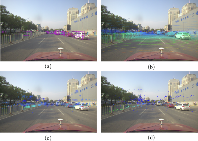
The configuration of our experiment platform and visualization scenarios on the data collected by different sensors. (a) shows information about the coordinate system of each sensor in the Ego Vehicle system. (b), (c), (d), and (e) show the results of the 3D bounding box annotations on the data (camera image, LiDAR point cloud, Arbe Phoenix point cloud, ARS548 RDI point cloud).
To validate the performance of different types of 4D radar in object detection and object tracking tasks and to fulfill researchers’ needs for a 4D radar dataset, we propose a novel dataset with two types of 4D radar point clouds. Collecting two types of 4D radar point clouds can explore the performance of point clouds with different sparsity levels for object detection in the same scenario, which will provide a basis for developing 4D radar research in the field of ego vehicles. Our dataset has been published and researchers such as Fan42, Gao43, and Li44 have cited our dataset for comparative analyses with contrasting other 4D radar datasets.
Our main contributions to this work are as follows:
(1) We present a dataset with multi-modal data, which includes camera data, LiDAR point cloud, and two types of 4D radar point cloud. Our dataset can study the performance of different types of 4D radar data, contributes to the study of perception algorithms that can process different types of 4D radar data, and can be used to study single-modal and multi-modal fusion tasks.
(2) Our dataset provides a variety of challenging scenarios, including scenarios with different road conditions (city and tunnel), different weather (sunny, cloudy, and adverse weather), different light intensities (normal light and backlight), different times of day (daytime, dusk, and nighttime), These scenarios can be used to assess the performance of different types of 4D radar point cloud in different scenarios.
(3) Our dataset consists of 151 continuous time sequences, most of which last 20 seconds. There are 10,007 frames carefully synchronized frames and 103,272 high-quality annotated objects.
Methods
In this section, we propose the main aspects of our dataset, including the sensor specification of the ego vehicle system, sensor calibration, dataset annotation, data collection and distribution, and the visualization of the dataset.
Sensor Specification
Our ego vehicle’s configuration and the coordinate relationships between multiple sensors are shown in Fig. 1. The platform of our ego vehicle system consists of a high-resolution camera, a new 80-line LiDAR, and two types of 4D radar. The sensor configurations are shown in Table 2. All sensors have been carefully calibrated. The camera and LiDAR are mounted directly above the ego vehicle, while the 4D radars are installed in front of it. Due to the range of horizontal view limitations of the camera and 4D radars, we collect data only from the front of our ego vehicle for annotation. The ARS548 RDI captures data within an approximately 120° horizontal field of view and 28° vertical field of view in front of the ego vehicle, while the Arbe Phoenix, operating in middle-range mode, collects data within a 100° horizontal field of view and 30° vertical field of view. The LiDAR collects around the ego vehicle in a 360° manner but only retains the data in the approximate 120° field of view in front of it for annotation. The specifications of the sensors are provided in Table 2.
Sensor Calibration
The calibration work for this dataset primarily includes camera-LiDAR joint calibration and camera-4D radar joint calibration, both conducted using offline calibration methods. The advantage of offline calibration lies in achieving spatial synchronization in a windless open environment, thereby minimizing spatial synchronization errors and obtaining more precise calibration parameters. Temporal synchronization between different sensors is achieved through hardware synchronization devices, which can provide high-precision timing based on GPS. Additionally, as some scenes in this experiment are derived from environments with weak communication capabilities (e.g., tunnels), offline calibration ensures that temporal synchronization is unaffected by environmental constraints. This allows the synchronization between different sensors to be reliably managed by hardware devices, ensuring the feasibility of the experimental data. Existing 3D radar calibration methods are based on LiDAR calibration techniques and have achieved good results by incorporating the unique characteristics of 3D radar. Therefore, the process of obtaining the internal and external parameters of 4D radar can follow and extend the calibration procedures for 3D radar. In this study, our calibration work is as follows: (1) By placing the calibration board at different positions within the common field of view of the 4D radar and the camera, at least six sets of calibration data are collected. Each set of calibration data includes RGB images from the camera and point cloud data from the 4D radar. One side of the calibration board facing the 4D radar and the camera features a checkerboard pattern, while the center of the other side is equipped with a corner reflector, whose imaging point serves as a feature point. (2) From each set of calibration data, the 3D coordinates of the feature points in the radar coordinate system and the 2D coordinates of the feature points in the camera coordinate system are extracted. (3) Using the correspondence between the 3D coordinates of the feature points in the radar coordinate system and the 2D coordinates in the camera coordinate system, a transformation equation is established. The transformation equation is then solved to obtain the calibration parameters for the 4D radar and the camera. (4) The calibration process for LiDAR and cameras is consistent with that for 4D radar and cameras. Both involve using a specific calibration board or device to collect multiple sets of data within the shared field of view of the two sensors. Feature points are then extracted, and coordinate transformations are performed to establish the spatial transformation relationship between the two sensors, thereby determining the calibration parameters between them. The point cloud projection relationship between the point clouds of the LiDAR and the two radars on the camera image in the same frame is shown in Fig. 2, where the LiDAR point cloud is the complete un-noise-cancelled point cloud data, the point cloud of the ARS548 RDI and the point cloud of the Arbe Phoenix.
Projection visualization of sensor calibration. (a), (b), (c), and (d) represent the projection of the calibrated data (camera image, LiDAR point cloud, Arbe Phoenix point cloud, and ARS548 RDI point cloud) on the image.
Dataset Annotation
In our dataset, we provide 3D bounding boxes, object labels, and tracking IDs for each object. The synchronized frames are annotated based on camera and LiDAR point clouds. The 3D bounding boxes are derived by projecting the LiDAR point cloud onto the camera images. We do not distinguish between objects in dynamic or static states during annotation. To synchronize the timestamps between different sensors, we choose the Precision Time Protocol (PTP) to align the time between multiple sensors using GPS message timing with time synchronization devices.
We provide basic information for each object within a 100-meter distance, including the relative coordinates (x, y, z) of the corresponding 3D bounding box, absolute dimensions (length, width, height), and the orientation angle (alpha) in the Bird’s Eye View (BEV), which requires careful calculation. To ensure the usability of the data, we also provide features for object occlusion and truncation. We annotated over ten categories of labels, with a focus on five primary categories, including “Car”, “Pedestrian”, “Cyclist”, “Bus” and “Truck”. The remaining labels are grouped as “Others”. According to statistics from the collected raw data, approximately 50,000 synchronized frames were extracted, and 10,007 frames were annotated among them. We annotated 103,272 objects from the annotated frames.
Methods for technical validation
We employed a server based on the Ubuntu 18.04 system as our hardware platform. We adopted the OpenPCDet project based on Pytorch 10.2, the batch size setting to the default value of 4, and each experiment was trained for 80 epochs at a learning rate of 0.003 on four Nvidia RTX3090 graphics cards. To demonstrate the performance of our dataset and the designed algorithms, we introduced some existing state-of-the-art algorithms, all carrying out experiments as required, we use five unimodal baseline models such as PointPillars45, Voxel R-CNN46, RDIoU47, CasA-V48, CasA-T48 and two multi-modal baseline models such as VFF49, M2-Fusion40.
Data Records
The dataset is available in both the data repositories50,51,52. Our image data is published as png images and Lidar point cloud and radar point cloud data is published as bin files, which are fully accessible to the user without any further licence. In this section, we describe the detailed contents and file directory of Dual Radar.
Dataset organization
We take three kinds of labels as the experiment objects, which are “Car”, “Pedestrian” and “Cyclist”. According to the need of the experiment, we split all the annotated data into a training, validation, and test set according to the ratio of 51%, 25%, and 24%. Our dataset will be published in the KITTI53 format.
We conducted statistical analysis on our dataset and summarized the total counts for each label, as shown in Fig. 3. We presented a pie chart to display the object counts of the top six labels. The “Car” label slightly exceeds 50% of the total object count. Most of our data was obtained in urban conditions with decent traffic roads. As a result, the majority of labels are concentrated in “Car”, “Cyclist” and “Pedestrian”. We choose objects from these three labels to validate the performance of our dataset. We further analyzed the frame counts under different weather conditions and periods, as shown in Fig. 4 and Table 3. About two-thirds of our data were collected under normal weather conditions, and about one-third were collected under adverse weather. We collected 577 frames in adverse weather, which is about 5.5% of the total dataset. The adverse weather data we collect can be used to test the performance of different 4D radars in adverse weather conditions.
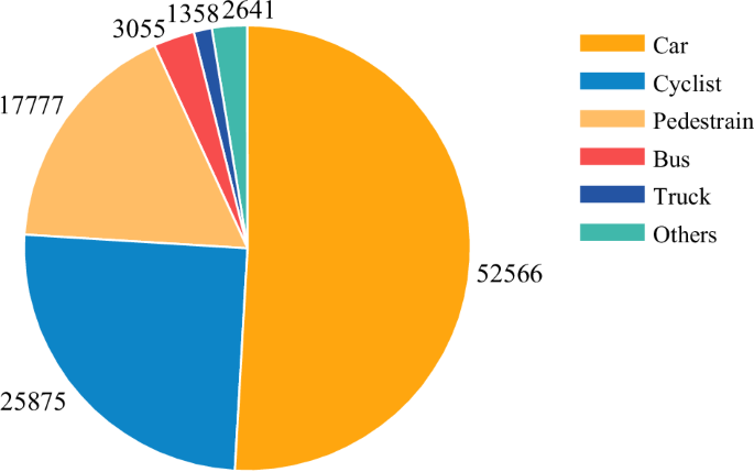
The statistics of the number of objects in different labels. The result suggests that the main labels like Car, Pedestrian, and Cyclist take up over three-quarters of the total amount of objects.
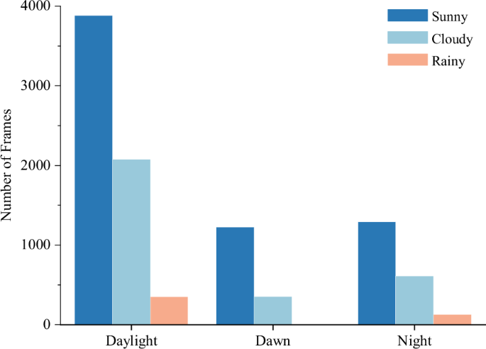
The statistics of the number of frames for various periods in different weather. Our dataset is classified into eight categories based on the weather conditions and periods.
We also collected data at dawn and night when low light intensity challenged the camera’s performance. We also conducted a statistical analysis of the number of objects with each label at different distance ranges from our vehicle, as shown in Fig. 5. Most objects are within 60 meters of our ego vehicle. The distribution of distances between “Bus”, “Truck” and our ego vehicle is uniform across each range. In addition, we analyzed the distribution density of the point clouds and the number of point clouds per frame, as shown in Fig. 6 and Table 4. In most cases, the LiDAR has 110K to 120K points per frame, the Arbe Phoenix radar has 6K to 14K points per frame, and the ARS548 RDI radar has 400 to 650 points per frame. Due to a lot of noise in the data collection set in the tunnel scenario, there will be part of the data with much larger than normal point clouds, as shown in 713 frames of LiDAR data with more than 130K point clouds and 158 frames of Arbe Phoenix radar data with more than 26K point clouds. Based on these statistical results, our dataset encompasses adverse driving scenarios, making it conducive for the application of objects like “Car”, “Pedestrian” and “Cyclist” in experiments. Moreover, the simultaneous collection of 4D radar point clouds from two types of 4D radar is useful for analyzing the effects of different 4D radar point clouds on specific driving scenarios and researching perceptual algorithms that can process different 4D radar point clouds. This dataset has significant implications for applying theoretical experiments in autonomous driving.
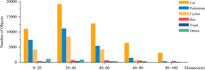
The statistic of different annotated objects at different ranges of distance from the ego vehicle. From the results, the majority of the annotated objects are in the range of 20m-60m. About 10% of the annotated objects are in the range of more than 60 m.

The statistics on the number of point clouds per data frame. (a) show that most LiDAR point cloud counts are between 110K and 120K. (b) show that Arbe Phoenix point cloud counts are between 6K and 14K. (c) show that ARS548 RDI point cloud counts are between 400 and 650.
Data Visualization
We visualize some of the data as shown in Figs. 7 and 8. Objects are annotated using 3D bounding boxes, which are mapped to the image, LiDAR point cloud, and two 4D radar point clouds. The 3D bounding box fits the object well and accurately depicts the corresponding points in the point cloud. Objects in both the LiDAR and 4D radar point clouds align well with those in the image, confirming good synchronization. The robustness of the 4D radar across different scenarios, weather conditions, and lighting conditions can be observed in Figs. 7 and 8. As shown in Fig. 8(g,h,i,j,k), the camera is highly affected by light and weather, and the camera image lacks RGB information to observe the object when the light is weak, backlit and adverse weather. In the corresponding scenarios, LiDAR acquires very tight spatial information, compensating for the camera’s shortcomings. However, the LiDAR cannot effectively distinguish overlapping or relatively close objects in scenarios with more objects. The Arbe Phoenix radar can collect a dense point cloud, which can collect all the objects within the field of view, but it contains much noise. The ARS548 RDI radar produces a less dense point cloud, with occasional detection leakage, but each point cloud accurately represents object information. The ARS548 RDI radar can also be used to collect the information of the object in the field of view.
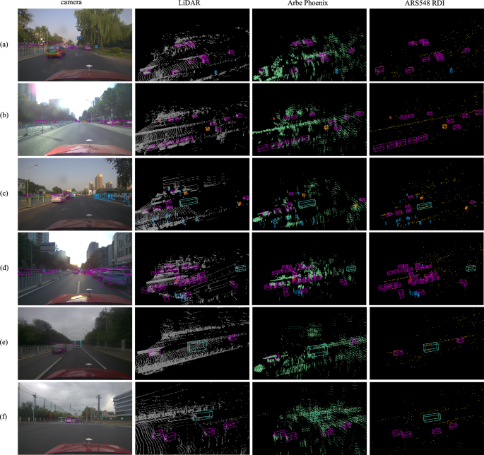
Representing 3D annotations in multiple scenarios and sensor modalities. The four columns respectively display the projection of 3D annotation boxes in images, LiDAR point clouds, Arbe Phoenix and ARS548 RDI radar point clouds. Each row represents a scenario type. (a) downtown daytime normal light; (b) downtown daytime backlight; (c) downtown dusk normal light; (d) downtown dusk backlight; (e) downtown clear night; (f) downtown daytime cloudy.

Representing 3D annotations in multiple scenarios and sensor modalities. Each row represents one scenario. (g) downtown adverse weather day; (h) downtown cloudy dusk; (i) downtown cloudy night; (j) downtown adverse weather night; (k) daytime tunnel; (l) nighttime tunnel.
Technical Validation
This section establishes the experimental platform for conducting the experiments on our dataset. We utilize several state-of-the-art baselines to validate our dataset. The performance of our dataset is verified by the results obtained from the experiments. We then conduct both qualitative and quantitative analyses on the results of the experiments, and finally, we get our evaluations of our dataset.
Experiments with our dataset in some single model
As shown in Table 5, the LiDAR point clouds captured in our dataset have excellent detection results, while the 4D radar point clouds have the potential for improvement. In the BEV view, the detection accuracies of the CasA-V model using the LiDAR point cloud reach 59.12% (Car), 49.35% (Pedestrian), and 50.03% (Cyclist), which indicates that the LiDAR point cloud in this dataset is able to represent the object information well. However, the detection accuracies are lower when using the 4D radar. In the BEV view, it can be observed that the CasA-V model achieves 12.28% and 3.74% in the “Car” category using the Arbe Phoenix and ARS548 RDI point clouds. This difference is due to the higher point density of the 80-line LiDAR, which collects much more information than the 4D radar. Meanwhile, the PointPillars model has achieved an accuracy of 35.09% in the category of “Car” when using the Arbe Phoenix radar point cloud, which is 26.95% higher than ARS548 RDI. This shows that despite the noise, the Arbe Phoenix radar point cloud can still represent the object information. The ARS548 RDI radar point cloud outperforms the Arbe Phoenix radar point cloud in the middle-sized “Cyclist” category. The accuracy of the PointPillars model on the ARS548 RDI radar point cloud reached 1.64% (Cyclist), which is 1.4% higher than the Arbe Phoenix radar point cloud. This is because cars with a large amount of metal are more conducive to collecting object information by LiDAR and radar. Although the Arbe Phoenix collects much noise, it can still better detect large metal objects. While the “Cyclist” object has less metal on it, collecting a lot of noise affects the model’s performance. The dataset label data defines the 3D bounding box through LiDAR point clouds, which cannot sometimes be captured by 4D radar because “pedestrian” objects usually have a smaller area, and 4D radar point clouds are sparser than LiDAR point clouds. The sparser nature of 4D radar point clouds compared to LiDAR point clouds can lead to situations where the radar does not detect the object, resulting in poor or even zero detection accuracy when training with 4D radar point clouds.
Experiments with our dataset in some multi-modal
In addition, we discuss the Detection performance of the multi-modal baseline model using this dataset. As can be seen in Table 6, when the M2-Fusion model fuses LiDAR and 4D radar, the detection of the “Car” category has a huge performance improvement. The detection results in the BEV view are higher than those of the other single-modal baseline models and 30.24% higher than the model of PointPillars. This indicates that the 4D radar data of this dataset can provide auxiliary information for LiDAR. Meanwhile, in the 3D view of the “Cyclist” category, when the LiDAR and ARS548 RDI radar point clouds are fused, the result is 4.72% higher than the result of fusing LiDAR and Arbe Phoenix radar point clouds, and 0.6% higher than the CasA-V model using only LiDAR point clouds. This further demonstrates the superior detection performance of the ARS548 RDI radar point cloud for the “Cyclist” category. Moreover, the experimental results of the VFF model using the camera image fused with the LiDAR point cloud are Significantly outperform than most single-modal baseline models. In the BEV view, the VFF model using images and LiDAR has 25.16% higher detection results than the CasA-V model using only LiDAR in the “Car” category, which suggests that the camera can provide rich information and can perform well after fusing with the spatial information of the point cloud.
Comparison of baseline models in adverse weather conditions
We compared the PointPillars and RDIoU models’ detection performance in adverse weather conditions. As can be seen in Table 7, the 4D radar performs better in adverse weather conditions. For the “Car” category, the RDIoU model has much higher detection results on radar point clouds than on LiDAR point clouds. The RDIoU model’s BEV and 3D view detection performance using the Arbe Phoenix radar point cloud is 14.78% and 10.27% better than LiDAR’s.
However, for the “Cyclist” and “Pedestrian” categories, both 4D radar point clouds did not achieve satisfactory results. The PointPillars model achieved excellent results on the ARS548 RDI point cloud, while the RDIoU achieved excellent results on the Arbe Phoenix point cloud gave better results. These experimental results show that this dataset’s two 4D radar point clouds show different performance characteristics. This provides data support for further research on using 4D radar point clouds with different point cloud densities and noise levels in adverse scenarios and contributes to developing algorithms that can perform well on different 4D radar point clouds.


Responses