Dynamic thermalization on noisy quantum hardware

The notions of temperature and statistics in isolated quantum systems are based on the mean and variance of a physical observable over repeated experiments^1,2. Microscopically, the emergence of statistical mechanics from the quantum description of a closed system is understood via thermalization. Thermalization implies that the quantum mechanical expectation value of the observable dynamically relaxes to the thermal one^3,4,5,6,7. Achieving thermalization requires the system to equilibrate: the expectation value of an observable ({{{mathcal{O}}}}) is stationary,

where (overline{rho }) is the time-averaged diagonal density matrix and the trace is taken over the entire system. In turn, the equilibrium expectation value (1) is thermal if it agrees with the one evaluated with the thermal density matrix ρ_th describing a Gibbs state,

Relaxation after a quench is one way thermal observables occur in a closed quantum system. The quench induces an interaction between the system’s subparts and initiates the dynamics. As a result, the system equilibrates (1) and thermalizes (2) unless it possesses extra constraints that, e.g., result in integrability or lead to many-body localization⁸.

In the present research, we demonstrate a mechanism for the occurrence of thermal observables and fluctuations in the course of post-quench dynamics, not relying on the presence of a thermal bath that ensures thermalization if the system is rather small. For an isolated system of several qubits (either interacting or non-interacting), we consider a quench protocol that turns on an all-to-all interaction with coupling constants sampled from a complex Gaussian distribution with zero mean and finite variance. The protocol is repeated multiple times with different sets of couplings. We find the equilibrium value of an observable dynamically arising from averaging over the realizations of the quench protocol:

The double brackets denote the quantum mechanical mean averaged over realizations, and t_eq is the time after which the observable becomes stationary. The observable equilibrates to the thermal value,

where the temperature T appears due to the quenched interaction and depends on the energy of the initial state ε_in. The system thermalizes to a positive or negative temperature state as it has a bounded spectrum and no kinetic energy⁹. The average thermal observables emerge irrespective of whether the pre-quenched Hamiltonian of the system is integrable or not. Below, we demonstrate this approach leads to thermal observables for the pre-quenched system without an external thermal bath.

We experimentally examine our thermalization mechanism (3,4) in a simulation on an IBM Quantum computer (IBMQ) for a system of four qubits. Upon equilibration, we read out the occupation probabilities of the many-body energy states of the system described by the pre-quench Hamiltonian. For the system’s initial state given by the ground state of the qubits, the average occupation probabilities relax to the Gibbs distribution. Starting from the highest excited state leads to the inversely populated state (T < 0). As a result, both the observables and their fluctuations evaluated from the noisy quantum computer’s error-mitigated output display thermal behavior with positive or negative absolute temperatures.

Being implemented on noisy intermediate-scale quantum (NISQ) hardware, our approach allows probing thermal observables in finite-size quantum systems in a highly controlled environment and may be utilized among nature-inspired quantum algorithms for thermal state preparation^10,11. Considerable experimental effort has been spent on sampling observables agreeing with the Gibbs state prediction on quantum computers. Analog or hybrid analog-digital devices allow simulating finite-temperature transitions for systems of  ~10–70 qubits^12,13, but with the trade-off of having no precise control over the target temperature and a lack of universality compared to their purely digital (gate-based) counterparts. In turn, some recent experiments on digital quantum computers are based on an imaginary time evolution algorithm^14,15 or an approach using thermofield double states^16,17, while another incorporates an infinite thermal bath using ancilla qubits¹¹. These experiments utilize ancilla qubits and achieve thermalization for relatively small systems of 2 to 4 qubits. Quantum-classical algorithms combining quantum simulations with classical data post-processing, matching quantum output with results expected from classical simulations, allow pushing this limit for larger systems of  ~ 8 qubits¹⁸. Here, we also address thermalization in a small system on a digital quantum computer. Typically, one assesses thermalization from the agreement of the observables measured at the end of the simulation with the Gibbs state prediction. We rely on the post-quench evolution and the averaging of observables over realizations of the randomized auxiliary interaction. Our protocol is inherently dynamical, enabling studying the formation of thermal observables in real time. Furthermore, it relies on the classical averaging of quantum observables corresponding to an individual realization of the quench protocol, unloading precious resources of the quantum computer. Advantageously, it does not require long-time evolution or increasing the system size due to auxiliary qubits aiming to simulate a thermal bath.

The paper is organized as follows. First, we define the quench protocol, introducing the auxiliary random interaction that governs post-quench evolution. Then, we derive thermal energies and occupation probabilities from the dynamic observables averaged over realizations of the auxiliary interaction for a system describing four non-interacting qubits before the quench. We demonstrate that the average total energy conservation respected in the evolution defines the temperature in the equilibrated observables, whilst the choice of the initial state defines the temperature’s sign. We use eigenstates of the pre-quenched Hamiltonian as the initial states. Second, we repeat the protocol for a more general case, where we choose a non-integrable Ising model as our pre-quenched Hamiltonian for eight qubits and begin with an arbitrary initial state. Despite the absence of a thermal bath, averaging the observables over random instances of the auxiliary interaction, we report that the energy fluctuations-to-energy ratio for the Ising Hamiltonian equilibrates to a value predicted by temperature determined by the conservation of total energy, reminiscent of fluctuation-dissipation theorem. Third, we run our thermalization protocol on a quantum computer for a system of four qubits, extracting thermal occupations, energies, and energy fluctuations corresponding to finite positive and negative temperatures. Each realization of the auxiliary interaction runs independently on the quantum computer while averaging is done classically upon readout. Implementing error-mitigation, we find that the hardware noise partly contributes to the temperature in the average simulated observables.

The model

Quenching a closed system is a natural way of probing its equilibration dynamics and subsequent thermalization¹⁹. For example, thermalization may occur via a non-linear classical mode and the development of turbulence, leading to eventual energy equipartition²⁰, or due to switching on a highly non-local interaction in a quantum system resulting in its equilibration to an infinite temperature state^21,22. Taking this dynamical perspective, we organize our quench protocol as follows.

We prepare N non-degenerate qubits in an eigenstate of ({H}_{0}= {sum }_{j = 1}^{N}({omega }_{j}/2),{sigma }_{j}^{y}): ({H}_{0}| {psi }_{{{{rm{in}}}}} rangle = {varepsilon }_{{{{rm{in}}}}}| {psi }_{{{{rm{in}}}}} rangle). Here ({sigma }_{j}^{y}) is the second Pauli matrix acting on the jth qubit, ω_j is the jth qubit’s frequency, (| {psi }_{{{{rm{in}}}}} rangle) is the initial state of the system, and ε_in is the corresponding eigenenergy. At time t = 0, we abruptly turn on a global quench that couples the qubits all-to-all and initiates the dynamics. The initial state (| {psi }_{{{{rm{in}}}}} rangle) starts evolving with the Hamiltonian

where

describes the interaction between the qubits with the coupling constants ({J}_{{j}_{1}{j}_{2}}) drawn from the Gaussian unitary ensemble with zero mean (langle {J}_{{j}_{1}{j}_{2}}rangle =0) and finite variance (langle | {J}_{{j}_{1}{j}_{2}}{| }^{2}rangle ={J}^{2}/N). Accordingly, one may understand the interaction term (6) as the Hamiltonian of random non-interacting fermions²³ projected onto the qubits’ basis via the Jordan-Wigner transform. While both H₀ and ({{{mathcal{V}}}}) are integrable, their combination is not. Indeed, when ({{{mathcal{V}}}}) is combined with H₀ in the full Hamiltonian (5), the latter is chaotic, displaying Wigner-Dyson level statistics²⁴ as discussed in more detail in the methods section. As such, the Hamiltonian (5) describes an interacting theory in fermionic or qubit representation, giving rise to the quantum many-body dynamics we address below.

We repeat the time evolution of the initial state (| {psi }_{{{{rm{in}}}}} rangle) with the Hamiltonian (5) for different sets of random couplings and compute quantum mechanical mean values averaged over realizations of the quench protocol, aiming to check the equilibration (3) and thermalization (4) conditions.

Once the interaction ({{{mathcal{V}}}}) is on, the evolving state (| psi (t) rangle ={e}^{-it({H}_{0}+{{{mathcal{V}}}})}| {psi }_{{{{rm{in}}}}} rangle) is no longer an eigenstate of H₀ whose expectation value (langle {H}_{0}(t)rangle =langle psi (t)| {H}_{0}| psi (t)rangle) becomes dynamic. To study the dynamics, we write ({H}_{0}={sum }_{l}{varepsilon }_{l}| l rangle langle l|) in the basis of its L = 2^N many-body energy eigenstates labeled by the index l, and average (langle {H}_{0}(t)rangle) over the protocol’s realizations. Thereby, we have

where

is the average occupation probability of the many-body state with energy ε_l for t > 0. Throughout the evolution, the total energy of the system is conserved on average, (langle langle H(t)rangle rangle =langle langle {psi }_{{{{rm{in}}}}}| H| {psi }_{{{{rm{in}}}}}rangle rangle ={varepsilon }_{{{{rm{in}}}}}), due to the zero mean of the Gaussian in Eq. (6).

Exact dynamics

Anticipating our quantum simulation experiment, we choose N = 4 and run the complete protocol numerically for different initial states (| {psi }_{{{{rm{in}}}}} rangle =| downarrow downarrow downarrow downarrow rangle), (| uparrow downarrow downarrow downarrow rangle), …, (| uparrow uparrow uparrow uparrow rangle), all having distinct initial energies, where the down arrow denotes a qubit in the ground state of ({sigma }_{j}^{y}) and the up arrow marks the excited state of a qubit.

As shown in Fig. 1a, the average expectation value (7) becomes stationary at t_eq ≈ 2.5/J up to small finite-size oscillations. On the contrary, the expectation value for each realization of random couplings persistently oscillates at high amplitude. The equilibration of the mean (7) appears along with the building up of the diagonal entropy, (S(t)=-{sum }_{l}langle langle {n}_{l}(t)rangle rangle ln langle langle {n}_{l}(t)rangle rangle), which agrees with the properties of the thermodynamic entropy²⁵ and approaches an average stationary value S(t > t_eq) in Fig. 1b. Alongside, in Fig. 1a, we note that the equilibrated observables depend on the choice of the initial state. To rule out the possibility that our simulation has reached a quasi-equilibrium steady state, such as prethermalization^26,27, rather than fully equilibrated, we explore the dynamics of the observables at times far exceeding t_eq. Even though prethermalization is often associated with a weak breaking of integrability, it was recently observed in a trapped ion system with no conserved charges²⁸. In this case, achieving eventual thermalization and losing the information of the initial state requires evolution up to a timescale of the inverse minimal level spacing²⁹. In Fig. 1c, we demonstrate that the average expectation value (7) persists at times far exceeding the inverse minimal many-body level spacing of H, indicating complete equilibration, yet remains dependent on the initial state, which reflects the average total energy conservation.

The qubits’ frequencies are ω_j = 0.28J,  0.38J,  0.63J,  0.86J. a Expectation value of H₀ for four initial states as a function of time after the quench. The solid blue and dashed red curves show (langle langle {H}_{0}(t)rangle rangle) for a given initial state, while the dim gray curves depict (langle {H}_{0}(t)rangle) for each single realization of the quench protocol. b Diagonal entropy production evaluated with the average occupation probabilities (8) for the same four initial states displayed by the solid blue and dashed red curves. The gray curves show the diagonal entropy, (-{sum }_{l}| langle l| psi (t)rangle {| }^{2}ln | langle l| psi (t)rangle {| }^{2}), for individual realizations of the quench protocol. c Average expectation value (langle langle {H}_{0}(t)rangle rangle) evolved at times beyond the inverse average minimal many-body level spacing of the Hamiltonian H, (delta {varepsilon }_{min }=0.07J). d Occupation probabilities upon equilibration after quenching the qubits prepared in the ground state (| {psi }_{{{{rm{in}}}}} rangle =| downarrow downarrow downarrow downarrow rangle) (left) and the highest excited state (| {psi }_{{{{rm{in}}}}} rangle =| uparrow uparrow uparrow uparrow rangle) (right). The blue squares are the average occupations (8) and the red dots show the thermal fit (9). e Kullback-Leibler divergence between the average occupation probabilities (8) and the Gibbs distribution (9) with temperature (T=overline{T}({varepsilon }_{{{{rm{in}}}}})). The inset shows the late-time behavior of the KL divergence in a log scale. f Equilibrium temperature (overline{T}({varepsilon }_{{{{rm{in}}}}})) as a function of the initial state’s energy. The fitted temperature’s error bar increases near the half-band as the system approaches the equally populated infinite temperature state. T_c denoted by empty squares is the temperature determined from the canonical ensemble and total energy conservation. g Blue squares show the diagonal entropy evaluated with the mean occupation probabilities (overline{ langle langle {n}_{l}rangle rangle }) averaged over the equilibrium time interval (from t = 2.5/J to t = 20/J) for all the initial states of the system. Red dots display the thermal entropy, ({S}_{{{{rm{th}}}}}=-{{{rm{Tr}}}}{rho }_{{{{rm{th}}}}}(overline{T}({varepsilon }_{{{{rm{in}}}}}))ln {rho }_{{{{rm{th}}}}}(overline{T}({varepsilon }_{{{{rm{in}}}}}))). We determine the error bars for the thermal data displayed by the red dots from the covariance of the thermal fit of the dynamical data shown by blue squares. The error bars for the dynamical occupations stem from standard errors of the average over realizations of ({{{mathcal{V}}}}) are within the size of the marker (blue squares).

Full size image

Having established equilibration (3), we explore the relaxation process further. Since the Hamiltonian (H={H}_{0}+{{{mathcal{V}}}}) is chaotic, it is natural to expect that the system equilibrates and thermalizes if it is large enough⁶. For a small system of N = 4 qubits, a dynamic observable averaged over an ensemble of realizations equilibrates after an interaction-dependent timescale t_eq, even though an observable computed with an individual realization of the quench protocol may severely oscillate. Generally, one can express the evolved state of the system as (| psi (t) rangle ={e}^{-i({H}_{0}+{{{mathcal{V}}}})t}| {psi }_{{{{rm{in}}}}} rangle ={sum }_{l}{c}_{l}(t)| l rangle), where we specifically choose the basis of eigenstates of the initial Hamiltonian H₀. Accordingly, the coefficients of this representation ({c}_{l}(t) = langle l| psi (t) rangle) are related to the probability of occupying the l-th state at time t: (langle {n}_{l}(t)rangle =| {c}_{l}(t){| }^{2}). For t > 0, these occupation probabilities begin to deviate from their initial values and become dynamically redistributed, evolving with the Hamiltonian (5). If the system equilibrates, the probabilities to occupy the l-th state of H₀ should become stationary, describing an equilibrium probability distribution. Here we check if the average occupation probabilities become thermal.

Generically, describing the equilibrium state of a quantum many-body system requires a generalized Gibbs ensemble to account for the conserved quantities. The generalized Gibbs ensemble reduces to the conventional Gibbs ensemble if the conserved quantities are limited to total energy, particle number, and momentum³⁰. Since our quench protocol respects only the total energy conservation on average, we compare the averaged occupation probabilities upon equilibration with those predicted by the usual Gibbs distribution:

By doing that, we aim to achieve thermal occupations for the initial system, assuming that the emergent temperature T absorbs the effects of the interaction. At t = 10/J > t_eq, we observe that while the occupation probabilities (langle {n}_{l}(t)rangle) stay irregular for each individual realization of the quench protocol, the average occupation probabilities (8) are well-approximated with the occupation probabilities ({n}_{l}^{{{{rm{th}}}}}(T)). To illustrate this agreement, we fit the average occupation probabilities (8) with the thermal ones (9) obeying the Gibbs distribution with the temperature T being a fitting parameter. We compare (langle langle {n}_{l}(t)rangle rangle) with the thermal fit ({n}_{l}^{{{{rm{th}}}}}(T)) in Fig. 1d.

As expected upon thermalization, the occupations depend on a single parameter – temperature, which, in our case, is set by the energy of the initial state. One may adjust the temperature’s absolute value by tuning the characteristic interaction strength, providing additional control over the thermalization process. The temperature retains the memory of the total energy persisting as a constraint throughout the relaxation, which makes the equilibrium observables initial-state-dependent. The choice of the initial state also defines the temperature’s sign, giving rise to negative absolute temperatures. Plotting the equilibrated mean occupation probabilities for the protocol started from the ground state (Fig. 1dleft) and the highest excited state (Fig. 1dright) of the qubits, we find a population inversion in the second case, which implies T < 0. While temperature is usually restricted to be non-negative for an unbounded energy spectrum to secure convergence of the partition function, negative absolute temperatures have been experimentally observed in systems with bounded spectra^{31,32,33,34,35,36,37,38,39}, as in our simulation.

To justify the quantitative agreement between the mean occupation probabilities and the Gibbs distribution, we consider the Kullback-Leibler (KL) divergence⁴⁰. The KL divergence serves as a measure of distance between the two probability distributions. It is non-negative by definition and equals zero only if the two probability distributions coincide. Since the average observables still possess small finite-size oscillations, as seen in Fig. 1a, to find the equilibrium temperature (overline{T}), we additionally average the mean occupations over a fixed time interval in the equilibrium regime (from t = 2.5/J to t = 20/J) and approximate the result with the thermal distribution (9) with (T=overline{T}). Then, we compare ({n}_{{{{rm{th}}}}}(overline{T})) with the dynamic occupations (8) via the KL divergence^41,42:

where (F(overline{T})=-overline{T}ln Z(overline{T})) is the thermodynamic free energy. For several initial states, we determine (overline{T}) and plot the KL divergence (10) as a function of time after the quench in Fig. 1e. The KL divergence decays for t > t_eq to the value  ~10⁻² which quantifies the accuracy of the thermal occupation probabilities.

Next, we evaluate the equilibrium temperature for 16 initial states given by the eigenstates of H₀. Due to energy conservation, if the system thermalizes, one may estimate the equilibrium temperature by matching the initial energy and a canonical ensemble prediction for the total energy:

where the angular brackets denote averaging over realizations of random couplings and H is the total Hamiltonian ({H}_{0}+{{{mathcal{V}}}}). Solving this equation gives the canonical prediction T_c for the temperature as a function of the initial energy. As seen in Fig. 1f, the equilibrium temperature (overline{T}) determined by fitting the average occupation probabilities in the equilibrium regime agrees well with the canonical temperature T_c. Analyzing the equilibrium temperature (overline{T}) versus the energy of the initial state ε_in in Fig. 1f, we observe that the equilibrium temperature is increasing as the initial state’s energy is increased up to the middle of the spectrum. A subsequent rise of the initial energy changes the equilibrium temperature from plus to minus infinity. Temperatures ± ∞ are equivalent and correspond to the maximum value of the thermal entropy that follows the semicircle-like function of the initial state’s energy, as shown in Fig. 1g. Increasing the energy above the half-band decreases the entropy, implying that the negative temperatures appear above T = + ∞ in the energy hierarchy^9,34.

So far, we have achieved thermal occupations of the many-body energy states for the system described by the Hamiltonian H₀ of four non-interacting qubits, starting the protocol from an eigenstate of H₀. To highlight the generality of our protocol, we choose the N = 8 Ising model with a periodic boundary condition, ({H}_{I}=-omega mathop{sum }_{j = 1}^{N}{sigma }_{j}^{x}-hmathop{sum }_{j = 1}^{N}{sigma }_{j}^{y} -gmathop{sum }_{j = 1}^{N-1}{sigma }_{j}^{y}{sigma }_{j+1}^{y}-g{sigma }_{N}^{y}{sigma }_{1}^{y}), as the initial Hamiltonian. We tune H_I to the paramagnetic phase (ω > h, g: ω = 0.15 J, h = 0.05 J, g = 0.1 J) and begin the evolution with a σ^y-ordered state, (| {psi }_{{{{rm{in}}}}} rangle =| uparrow uparrow ldots uparrow rangle), which is not an eigenstate of H_I. In Fig. 2a, we plot the ratio of the energy fluctuations, ({{{rm{Var}}}}{H}_{I}=langle langle {H}_{I}{(t)}^{2}rangle rangle -{langle langle {H}_{I}(t)rangle rangle }^{2}), to the mean energy (langle langle {H}_{I}(t)rangle rangle) in the initial system, reminiscent of a fluctuation-dissipation relation for thermal systems, where we average over one hundred realizations of random couplings in the quenched interaction ({{{mathcal{V}}}}). The energy fluctuations-to-energy ratio equilibrates and remains stationary up to weak oscillations In Fig. 2b, we show the average occupation probabilities (additionally time-averaged over the equilibrium regime from t = 10/J to t = 500/J). As in the case of the non-interacting initial Hamiltonian, we fit the average occupation probabilities by the Gibbs state’s prediction (9) to determine the equilibrium temperature (overline{T}). We also determine the canonical temperature T_c from the total energy conservation (11). Both temperatures agree within the error bar, as seen in Fig. 2b, where we plotted the Gibbs distributed occupations of H_I with the temperature T_c with a dash-dotted black curve on top of the averaged data (blue squares) and the thermal fit (red circles). The average occupation probabilities are well-described by the thermal ensemble except for the edges of the spectrum, expected for a finite-size system. However, the temperature found in both ways is sufficient to correctly predict the equilibrium value of the energy fluctuations-to-energy ratio for H_I, as seen in Fig. 2a. We find the thermal values of the energy fluctuations-to-energy ratio from the thermal averages: ({langle {H}_{I}rangle }_{{{{rm{th}}}}}=mathop{sum }_{l = 1}^{L-1}{n}_{l}^{{{{rm{th}}}}}(T){varepsilon }_{l}) and ({{{{rm{Var}}}}}_{{{{rm{th}}}}},{H}_{I}=mathop{sum }_{l = 1}^{L-1}{n}_{l}^{{{{rm{th}}}}}(T){varepsilon }_{l}^{2}-{langle {H}_{I}rangle }_{{{{rm{th}}}}}^{2}) with (T=overline{T}), T_c, where ε_l are eigenenergies of H_I. Note that the spectrum of H_I has multiple degeneracies. We show the corresponding thermal values by two horizontal lines in Fig. 2a. The dash-dotted black line (T = T_c) lies right atop the dashed red line ((T=overline{T})). The thermal predictions agree with the equilibrated energy fluctuations-to-energy ratio obtained in the exact dynamics, highlighting that our protocol leads to the thermal behavior of energy fluctuations and energy of the initial system as expected from the fluctuation-dissipation theorem. Finally, in Fig. 2c, we show the KL divergence (10) between the mean dynamic occupations and Gibbs distribution with the equilibrium temperature (overline{T}). As seen in insets in Fig. 2c, the KL divergence equilibrates to values  ~10⁻² in time (sim {{{mathcal{O}}}}(1)/J), qualitatively similar to our analysis for the non-interacting initial system. Despite increasing the system size, we still find that the system equilibrates in ({t}_{{{{rm{eq}}}}} sim {{{mathcal{O}}}}(1)/J).

a Energy fluctuations-to-energy ratio of H_I as a function of time after quenching ({{{mathcal{V}}}}). Horizontal lines show thermal predictions of the energy fluctuations-to-energy ratio, with temperatures determined from fitting the mean occupation probabilities averaged over time in the equilibrium regime ((overline{T})) and from total energy conservation (T_c). (delta {epsilon }_{min }approx 0.00254J) is the average minimal level spacing of the full Hamiltonian H. b Mean occupation probabilities for eigenstates of H_I, time-averaged over the equilibrium regime, in log scale. Blue squares are dynamical occupations averaged over 100 realizations of random couplings and time (from t = 10/J to t = 500/J). The error bars are standard errors accumulated when averaging over realizations of ({{{mathcal{V}}}}), averaged over the equilibrium time interval. Red dots represent the thermal fit of the averaged dynamical data. The error bars are found from the square root of the covariance of the fitting parameters and are within the size of the marker. The dash-dotted black line shows thermal occupations with temperature determined by the total energy conservation (11). c Kullback-Leibler (KL) divergence between mean occupation probabilities (8) and thermal occupations with equilibrium temperature (overline{T}). The top inset shows the first five time points of the KL divergence, illustrating that it approaches the equilibrium value in (t sim {{{mathcal{O}}}}(1)/J). The bottom inset shows the KL divergence along the equilibrium time interval.

Full size image

Even for a small system, thermalization to a finite positive or negative temperature equilibrium occurs from the post-quench dynamics of a quantum system within the time scale (sim {{{mathcal{O}}}}(1)/J). Suitability for a small system, controllable equilibration timescale, and a lack of a thermostat make our thermalization mechanism possible to test experimentally on NISQ computers like IBMQ. Indeed, as we demonstrate below, executing the evolution of the interacting four-qubit system, described by the Hamiltonian (5), is viable on IBMQ with a moderate number of two-qubit gates, which is often the main limiting factor in studying many-body physics on NISQ devices. Achieving thermal observables relies on averaging the expectation values, which can be done classically from the output of every realization of the quench protocol, each running independently on a quantum computer.

Quantum simulation

We implement our dynamic thermalization protocol on an IBM Quantum computer (IBMQ) named ibm_hanoi for 100 realizations of the quench protocol, each corresponding to a quantum circuit. Encoding quantum dynamics into a quantum circuit implies applying a sequence of single- and two-qubit gates that approximate a given realization of the evolution operator (U(t)={e}^{-it({H}_{0}+{{{mathcal{V}}}})}) to the initial state (| {psi }_{{{{rm{in}}}}} rangle). Executing a quantum circuit on IBMQ is noise-susceptible, mostly due to the imperfect application of two-qubit gates, namely, CNOT gates that perform entangling operations between qubits in our simulation. Hence, our strategy to mitigate the error accumulated due to noise is: first, decreasing the number of CNOT gates required to perform the simulation as much as possible; second, simplifying the noise’s structure from the remaining CNOT gates and accounting for it in the simulation results.

To fulfill the first task, we adapt variational circuit recompilation^43,44 to approximate the evolution operator U(t) by a parametrized quantum circuit with 99.8% accuracy, optimizing the tensor network decomposition of U(t), before plugging it into the quantum computer. Using this method, we reduce the number of CNOT gates required for the simulation to N_CNOT = 60, discarding the need for Trotterization, which allows us to reach arbitrary times.

We address the second task using an extension of the randomized compiling (RC) approach⁴⁵ converting the noise, not only on qubits to which a CNOT gate is applied but also on the neighboring qubits, to an incoherent noise channel. The incoherent noise contains local and global components, where the latter acts uniformly on every qubit in the circuit. To account for the global incoherent noise, we approximate the noisy quantum computer’s output for average occupation probabilities (8) upon equilibration as a weighted mixture of the average occupations unaffected by the global incoherent noise and a uniform distribution describing a maximally mixed (infinite temperature) state. Aiming to see if the observables evaluated on the quantum computer display thermal behavior, we chose the average occupations unaffected by the global incoherent noise in the form of the finite temperature Gibbs distribution (9) so that the noisy average occupation probabilities read

The consistency of this choice settles by fitting the noisy quantum computer’s data to the model (12) where the temperature T and the circuit’s fidelity ({f}^{{N}_{{{{rm{CNOT}}}}}}) play a role of the fitting parameters.

In Fig. 3, we show the data for the average occupation probabilities evolved up to t = 10/J > t_eq for two initial states (| {psi }_{{{{rm{in}}}}} rangle =| downarrow downarrow downarrow downarrow rangle ,| uparrow uparrow uparrow uparrow rangle). For (| {psi }_{{{{rm{in}}}}} rangle =| downarrow downarrow downarrow downarrow rangle), in Fig. 3a, we notice that the average occupation probabilities obtained from the quantum computer (QC) deviate from the characteristic exponential shape of the Gibbs distribution fitted to the result for the exact dynamics (ED). However, the QC data is well-approximated by the two-parameters function (12), as seen from the solid blue fitting curve. Extracting the temperature from fitting the QC data to the model (12), we plot the corresponding thermal occupations (9) in Fig. 3b.

The evolution goes up to t = 10/J. a Occupation probabilities averaged over 100 realizations of the quench protocol with the initial state (| {psi }_{{{{rm{in}}}}} rangle =| downarrow downarrow downarrow downarrow rangle): the gray crosses display the result of the exact dynamics (ED); the dash-dotted gray line is the thermal fit (9) of the ED data; the blue circles show the outcome of the simulation on the quantum computer (QC) after error mitigation; the solid blue curve is the fit of the QC data with the model for noisy occupations (12); the red diamonds and the dashed red curve show the same as QC but with tripled noise amplification (QC3). b The Gibbs distribution for occupation probabilities (9) with the temperatures determined from fitting the ED and quantum simulation data in the (a). The error bars for QC and QC3 data sets in (a, b) are within the size of the designated symbols. ZNE refers to the temperature value obtained with zero-noise extrapolation for β = 1/T shown in the (c). d–f are analogous to (a–c) but for the protocol starting with (| {psi }_{{{{rm{in}}}}} rangle =| uparrow uparrow uparrow uparrow rangle). mQC3 is the mirror image of the QC3 value of the inverse temperature β = 1/T relative to the QC value of β, necessary for mirrored zero-noise extrapolation (mZNE) illustrated with the dashed magenta line in the (f). The frequencies of the qubits are the same as in Fig. 1. The plots for occupation probabilities are in the log scale along the y-axis. The error bars for the occupation probabilities in ED arise due to the finite sampling of the M = 100 realizations of the auxiliary interaction ({{{mathcal{V}}}}). We determine the error bars from the standard error: ({sigma }_{{{{rm{ED}}}}}={sigma }_{{{{mathcal{V}}}}}/sqrt{M}), where ({sigma }_{{{{mathcal{V}}}}}) is the standard deviation of the distribution. For the QC data, error bars additionally account for the finite sampling of randomized compiled (RC) circuits and shots. In this case, they are given by: ({sigma }_{{{{rm{QC}}}}}={({sigma }_{{{{mathcal{V}}}}}^{2}/M+ langle {sigma }_{{{{rm{RC+shot}}}}}^{2}rangle /M)}^{1/2}), where (langle ldots rangle) denotes the average over realizations of random couplings, and ({sigma }_{,{mbox{RC+shot}},}^{2}) is computed as described in Appendix E of ref. ⁴⁵. We find the error bars for inverse temperatures from the covariance of the thermal fit of the quantum data after averaging it over realizations of random couplings and applying preliminary error mitigation (such as RC and removing global depolarizing noise).

Full size image

The temperature obtained from the quantum simulation is higher than the temperature from the thermal prediction of the exact dynamics, as we observe from the occupations’ slopes in Fig. 3b. We attribute this heat-up to the part of the hardware noise so far unattended. Indeed, above, we have discussed the effect of the global incoherent noise, yet the local incoherent noise may be present in the system. We account for the remaining noise using the zero-noise extrapolation (ZNE) method^{46,47,48,49,50,51}, which involves repeating the experiment with artificially amplified noise and extrapolating the measurement results to the noiseless limit. For incoherent noise, a linear change in noise amplification generally leads to exponential change in an observable⁴⁸. From this perspective, the inverse temperature β = 1/T in the exponent of thermal occupations in Eq. (12) may absorb the impact of the remaining noise. Elaborating on this observation, we repeat the experiment with the tripled noise by tripling every CNOT gate in the circuit. The average occupation probabilities in the quantum simulation with tripled noise amplification (QC3) remain well within the incoherent noise approximation, (12) as shown in Fig. 3a. In turn, the temperature determined from the QC3 data (see Fig. 3b) increases further compared to the QC result, highlighting how the hardware noise on NISQ devices can lead to the temperature rise in the simulated observables. In Fig. 3c, we extrapolate the inverse temperature to the noiseless case using a linear fit based on two noise amplification values (QC, QC3). As the inverse temperature appears in the exponent of the noisy occupations (12), our method effectively performs an exponential extrapolation on the observables after clearing the effect of the global incoherent noise from the quantum data. As a result, the value of β_ZNE = (1.29 ± 0.12)/J determined from ZNE lies within the error bar with β_ED = (1.21 ± 0.04)/J found from fitting the occupations computed in the exact dynamics with the Gibbs distribution (9). The canonical prediction for β_c = 1/T_c = 1.20/J based on energy conservation well agrees with exact dynamics and experimental value of the inverse temperature upon error mitigation.

The state evolved from the highest energy state, (| {psi }_{{{{rm{in}}}}} rangle =| uparrow uparrow uparrow uparrow rangle), equilibrates to the inversely populated state in the quantum simulation as it does for the exact dynamics, with the QC results well-described by the noisy occupation probabilities (12) with T < 0, as shown in Fig. 3d, e. Tripling the noise on the quantum computer leads to the system’s equilibration to a state with T > 0. Indeed, negative temperature states are unstable when interacting with an environment⁹, which makes them particularly challenging to prepare. Since negative absolute temperatures are hotter than T = + ∞, with T = 0⁻ being the hottest^9,34, from a thermodynamic standpoint, the environment (considered at T > 0) cools the system at T < 0 to a positive temperature. Thinking of the hardware noise as a consequence of a quantum computer being an open system, one expects the inverse populations to be unstable against noise, as we observe for the QC3 occupation probabilities in Fig. 3d, e. However, in our case, the noise plays a substantial role in the dynamic formation of the system’s equilibrium state, being determined by the hardware and the circuit layout rather than describing an independent thermal entity interacting with the system equilibrated to a negative absolute temperature. Hence, it is hard to predict a threshold noise preserving T < 0 equilibrium. Therefore, performing zero-noise extrapolation to the noiseless negative temperature case requires caution. Upon tripling the noise, the temperature crosses infinity (β = 0) and has a high positive value (small positive β), implying cooling the system. Thereby, ZNE for the QC and QC3 inverse temperatures predicts the value of β_ZNE = (−4.74 ±  0.37)/J quite distant from the ED result, β_ED = (−1.25 ± 0.04)/J, in Fig. 3f. To extrapolate to the regime of a closed system, we take a heuristic approach and assume that the increasing noise heats the system monotonically, restricting T to the T < 0 sector and preventing relaxation to T > 0 equilibrium. In this way, we account for Δβ = ∣β_QC − β_QC3∣ and mirror the QC3 data point relative to the QC accordingly. Then we apply ZNE for the mirrored QC3 (mQC3) and QC points, shown in the dashed magenta line in Fig. 3f. The value of β_mZNE = (−1.15 ± 0.41)/J determined with this mirrored ZNE (mZNE) method is within the error bar from the result of the exact dynamics.

Having obtained the average thermal occupation probabilities in the zero-noise limit, we check if the quantum computer predicts thermal values of the dynamic observables in the equilibrium regime. We repeat the protocol for times t = {2.5, 5, 10}/J and compare the IBMQ results with the exact dynamics and the thermal approximation of ED (ED_β) for the average expectation value (langle langle {H}_{0}(t)rangle rangle) and its fluctuations (sqrt{{{{rm{Var}}}}{H}_{0}}=sqrt{langle langle {H}_{0}{(t)}^{2}rangle rangle -{langle langle {H}_{0}(t)rangle rangle }^{2}}). For the quench protocol started with the ground state of H₀, (| {psi }_{{{{rm{in}}}}} rangle =| downarrow downarrow downarrow downarrow rangle), the mean expectation value (7) computed with the thermal occupations predicted by the quantum computer agrees with the ED and ED_β results within the error bars, as seen in Fig. 4a. As for the fluctuations of H₀ shown in Fig. 4b, the quantum computer’s effective output lies right on the thermal curve, indicating that the fluctuations computed on a quantum computer are closer to the thermal equilibrium value than the prediction of the exact dynamics. For (| {psi }_{{{{rm{in}}}}} rangle =| uparrow uparrow uparrow uparrow rangle), the quantum computer predicts negative temperatures upon equilibration. In Fig. 4c, d, we demonstrate that the IBMQ output provides for (langle langle {H}_{0}rangle rangle) and (sqrt{{{{rm{Var}}}}{H}_{0}}) within the error bars from both ED and ED_β predictions for T < 0 regime.

a Average expectation value of H₀ for (| {psi }_{{{{rm{in}}}}} rangle =| downarrow downarrow downarrow downarrow rangle). ED denotes the exact dynamics, ED_β approximates the ED curve with the thermal fit, and ZNE refers to the observables computed with thermal occupations obtained from the quantum computer in the zero-noise limit. b Fluctuations of H₀, (sqrt{ langle langle {H}_{0}^{2}(t)rangle rangle -{ langle langle {H}_{0}(t)rangle rangle }^{2}}), for (| {psi }_{{{{rm{in}}}}} rangle =| downarrow downarrow downarrow downarrow rangle). c, d show the same as in (a, b) but for the different initial state, (| {psi }_{{{{rm{in}}}}} rangle =| uparrow uparrow uparrow uparrow rangle). mZNE designates the observables computed with the output of the mirrored ZNE approach we used to establish the zero-noise limit for states with negative temperatures. We compute the error bars for the quantum prediction of the mean energy from the uncertainty on the value of the inverse temperature β_ZNE (or β_mZNE) found from the thermal fit in Fig. 3: ({sigma }_{{H}_{0}}={sigma }_{{{{rm{(m)ZNE}}}}}sqrt{{{{{rm{Var}}}}}_{{{{rm{th}}}}}{H}_{0}}), where ({{{{rm{Var}}}}}_{{{{rm{th}}}}}{H}_{0}={ langle {H}_{0}^{2}rangle }_{{{{rm{th}}}}}-{ langle {H}_{0}rangle }_{{{{rm{th}}}}}^{2}={sum }_{l}{n}_{l}^{{{{rm{th}}}}}(T){epsilon }_{l}^{2}-{(mathop{sum }_{l = 0}^{L-1}{n}_{l}^{{{{rm{th}}}}}(T){epsilon }_{l})}^{2}) is the thermal energy variance at T = 1/β_(m)ZNE and ϵ_l are the eigenenergies of H₀. Similarly, for the energy fluctuations, we use ({sigma }_{sqrt{{{{rm{V; ar}}}}{H}_{0}}}={sigma }_{{{{rm{(m)ZNE}}}}}| { langle {({H}_{0}-{ langle {H}_{0}rangle }_{{{{rm{th}}}}})}^{3}rangle }_{{{{rm{th}}}}}| /(2sqrt{{{{{rm{Var}}}}}_{{{{rm{th}}}}}{H}_{0}})).

Full size image

We show how thermal observables can dynamically emerge in a closed quantum system as a result of averaging over repeated instances of a global quench initializing Gaussian random non-local interactions between the system’s subparts. After the quench, the system pursues evolution governed by the chaotic Hamiltonian falling into the class of Gaussian unitary ensemble of random matrices. Averaging the observables over many realizations of the quench protocol leads to their equilibration (3) and thermalization (4) in time ({t}_{{{{rm{eq}}}}} sim {{{mathcal{O}}}}(1)/J), where J is the characteristic interaction strength. The resulting averaged probabilities of occupying eigenstates of the initial system in the equilibrium regime, t > t_eq, follow the Gibbs distribution with positive or negative absolute temperatures depending on the initial state’s energy, conserved on average in the course of after-the-quench dynamics. One can additionally tune the absolute value of equilibrium temperature by adjusting the interaction strength J. This dynamic thermalization is particularly convenient to examine on NISQ devices such as IBMQ since it does not rely on the long-time evolution, large system size, or auxiliary qubits to emulate a thermostat but solely on the repetition of the quench protocol with different sets of random coupling constants.

Adapting the established error-mitigation techniques, we implement our thermalization protocol on the IBMQ machine using a circuit depth of 60 CNOT gates. We obtain thermal occupations for the sixteen many-body energy states of the four-qubit system, populated according to positive or negative absolute temperatures depending on the choice of the initial state. Respectively, the observables and their fluctuations found in quantum simulation agree with the thermal predictions. This utility of the digital quantum simulator for producing thermal observables may be attributed to the notion of the quantum computer as an open system and our implementation of the thermalization protocol. First, we average the expectation values over realizations of the quench protocol aiming at mimicking the thermodynamic limit and facilitating thermalization in a relatively small system. One way to think of thermalization in a small system is to consider it as a subpart of a much bigger system in the thermodynamic limit, with the rest of the system acting as a thermal bath. A recent observation notes that averaging the evolution of a system with randomized interaction results in effective dissipative dynamics²². Another recent study shows that adding a disorder in a simulated system in analog quantum simulations substantially reduces the necessary size of a bath for infinite temperature deep thermalization⁵². In our case, the finite temperature in the equilibrated observables relies on the property of the auxiliary interaction that respects the system’s total energy conservation on average in the quench protocol. In our experiment, we start with a pure state and observe dynamical relaxation to a finite temperature equilibrium for averaged observables without involving a thermal bath, with the mitigated noise seemingly falling into the same effectively dissipative channel and raising the temperature of the simulated observables. Second, we apply zero-noise extrapolation that resembles taking a dissipationless limit in an open quantum system. Genuinely, these two limits are non-commutative, and their correct order, naturally implemented in our protocol, may be essential to justify the occurrence of the fluctuation-dissipation theorem in a quantum system⁵³. Exploring this issue numerically for the Ising model as the initial Hamiltonian in our protocol, we find that the energy fluctuations-to-energy ratio equilibrates to the value predicted by temperature determined from the total energy conservation, resembling a fluctuation-dissipation relation for thermal systems. Alongside, in our simulation, the time for the observables to equilibrate is ({{{mathcal{O}}}}(1)/J), similar to the timescale of irreversible dynamics T₃ in an open quantum system, after which an unconstrained system thermalizes⁵⁴.

The advantage of the considered quench protocol is its inherently dynamic nature, which allows studying the occurrence of thermalization or, potentially, ergodicity breaking in quantum systems in real-time, efficiently engaging the limited resources of NISQ processors. We apply our quench protocol to study the emergence of the negative absolute temperature equilibrium on a digital quantum platform. While absolute temperatures are usually restricted to positive values due to kinetic energy, equilibrium at negative absolute temperatures is possible under certain conditions, in systems with a bounded energy spectrum. Bringing negative absolute temperature equilibrium states to reality inspired significant experimental efforts due to their non-trivial thermodynamic properties, e.g., losing entropy when absorbing energy. By now, negative temperature states were experimentally observed in a few physical systems such as nuclear spins^31,32, cold atoms^33,34,37, two-dimensional quantum superfluids^35,36, optical fibers³⁸, and a two-level system environment in superconducting qubits³⁹. Here, we present an equilibrium state with negative absolute temperature arising from the relaxation process in a quantum system realized digitally on a quantum computer.

Here, we discuss the choice of the thermalization protocol and describe various techniques we use to produce and analyze experimental data.

Choice of thermalization protocol

The choice of the interaction is essential for our protocol so that there would be no constraints preventing thermalization after the quench. We began with a “constrained” non-interacting Hamiltonian H₀ that can not be the sole source of thermalization dynamics. In our case, thermalization occurs due to the quenched random interaction ({{{mathcal{V}}}}) (with zero mean strength) between the qubits. Owing to the zero mean strength interaction, adding the latter to the initial Hamiltonian conserves only the total energy equal to the initial energy of the system on average. The inter-qubit interaction (6) maps onto the random free fermions, also known as the SYK₂ model, an explicitly non-interacting theory. However, the combined Hamiltonian (H={H}_{0}+{{{mathcal{V}}}}) is non-integrable, as may be seen from its level statistics.

The notion of energy level statistics allows characterizing integrability, localization, and chaos in quantum many-body systems. Chaotic behavior, closely related to thermalization⁶, manifests in statistical properties of a system’s many-body energy levels, falling in the Wigner-Dyson statistics described by a Gaussian orthogonal (GOE), unitary (GUE), or symplectic (GSE) ensemble of random matrices⁵⁵. On the contrary, integrability and localization are associated with level statistics following a Poisson distribution⁵⁶. Accordingly, changing disorder in a system may lead to a localization transition from Wigner-Dyson to Poisson level statistics^{57,58,59,60,61,62}.

To quantify the level statistics in our model, we use the probability distribution for a ratio 0≤r_l≤1 determined from two consecutive level spacings in a given part of a many-body spectrum⁵⁷: ({r}_{l}=min {{delta }_{l+1},{delta }_{l}}/max {{delta }_{l+1},{delta }_{l}}), where ({delta }_{l}={tilde{varepsilon }}_{l+1}-{tilde{varepsilon }}_{l}). Note that here ({tilde{varepsilon }}_{l}) are the eigenvalues of H. For the adjacent gap ratio r_l following Wigner-Dyson statistics, the probability distribution is (P(r)=2{(1+r)}^{beta }/{(1+r+{r}^{2})}^{1+frac{3beta }{2}}/{Z}_{beta }) with Z_β being a normalization constant and β is a symmetry index (do not confuse with an inverse temperature) equal to 1, 2, and 4 for GOE, GUE, and GSE, predicting mean values of the gap ratio ({langle rrangle }_{{{{rm{GOE}}}}}approx 0.54), ({langle rrangle }_{{{{rm{GUE}}}}}approx 0.6), and ({langle rrangle }_{{{{rm{GSE}}}}}approx 0.68)⁵⁹. In the integrable case, for the Poisson spectrum, the distribution of the gap ratio is P(r) = 2/(1+r)² with ({langle rrangle }_{{{{rm{Poisson}}}}}approx 0.39)⁵⁷. Following earlier studies^{57,58,59,60,61,62}, we consider our total Hamiltonian (H={H}_{0}+{{{mathcal{V}}}}) in the regime when the system is large enough (N = 10 with 2^N many-body energy levels) and plot the histogram for the gap ratio distribution for M = 1000 disorder realizations averaged over  ~10% of levels in Fig. 5. The distribution function is in complete agreement with GUE prediction and reproduces the mean adjacent gap ratio ({langle rrangle }_{{{{rm{GUE}}}}}approx 0.6). Reducing the system’s size and the number of realizations to what we use in our experiment and choosing the parameters accordingly, we observe that the level statistics of the model remain well-described by GUE in Fig. 5, highlighting an absence of integrability or localization.

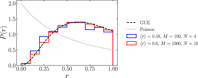
The blue histogram shows the probability distribution for a system of N = 4 qubits with the same M = 100 realizations we use for exact and quantum dynamics. We display the data averaged over 12 ratios of consequential level spacings without two pairs of states at the edges of the spectrum. The red histogram is done for the system with N = 10 qubits over M = 1000 realizations, averaging the data over  ~10% out of 2¹⁰ of many-body energy levels. For comparison, the black dashed line shows the Gaussian unitary ensemble (GUE) predicted level statistics. The gray dotted line displays Poisson (integrable) behavior put for a visual reference. Both (N = 4, M = 100) and (N = 10, M = 1000) datasets saturate the GUE curve and possess the GUE characteristic value of the mean adjacent gap ratio ({ langle rrangle }_{{{{rm{GUE}}}}}approx 0.6).

Full size image

Having established that the model is chaotic, i.e., described by a random matrix theory, one expects the observables evolved with the Hamiltonian H to equilibrate and thermalize. However, one realization of random couplings may not be enough for equilibration. In Fig. 6, we show the after-the-quench equilibration process for (langle {H}_{0}(t)rangle) for different system sizes (N = 4, 6, 8), averaging the expectation values with several numbers of realizations M = 10, 20, 100. Increasing the number of realizations leads to less finite-size oscillations in the average observable in the equilibrium regime. The larger the system, the fewer disorder realizations are needed to suppress the remaining oscillations in the observable.

We plot the expectation value of H₀ as a function of time for individual realizations of random couplings (gray curves), averaged over M = 100 realizations (solid blue curve), averaged over M = 10 realizations (dash-dotted green curve), and averaged over M = 20 realizations (dashed red curve) for different system sizes: (a) for N = 4 qubits, (b) for N  = 6 qubits, and (c) N = 8 qubits. The vertical black line marks the equilibration timescale at t = 2.5/J.

Full size image

Equilibration in the system results in thermal observables. In particular, we use the probabilities to occupy the many-body energy eigenstates of the initial Hamiltonian H₀. After the quench, the average occupation probabilities relax to a finite-temperature Gibbs distribution. This protocol allows for dynamically obtaining equilibrium observables at finite temperatures for a given system on a digital quantum processor without simulating a thermal bath.

Quantum simulation methods

Simulating the time evolution of a quantum-mechanical system on noisy NISQ devices, like IBMQ quantum computers, is susceptible to noise, generating output errors due to multiple sources. On IBMQ devices, it is known that errors stem principally from imperfect measurements, and from the application of imperfect two-qubit entangling gates, in our case, CNOT gates.

Variational circuit recompilation

On IBMQ devices, errors largely originate from the application of noisy CNOT gates associated with an error rate of  ~1%. A naive compilation of the unitary operator U(t) into a quantum circuit using, e.g., Qiskit’s transpile function⁶³ on a linear qubit layout yields a quantum circuit with as much as 238 CNOT gates, which would result in a global error rate close to 100%. This number of entangling gates originates from the all-to-all interaction (6) essential for our thermalization mechanism. To minimize the number of noisy CNOT gates required for the simulation, we take an alternative approach to recompile our quantum circuits, adapting a variational approach similar to the one presented in refs. ^43,44, which has already shown promising results on NISQ devices^64,65,66. The general idea of the method is to consider an ansatz quantum circuit with a given CNOT gate structure and parametrized single-qubit gates and optimize these parameters until the circuit implements a suitable approximation of the target unitary U(t). For few-qubits circuits, the optimization is done on a classical computer using a tensor network decomposition of both the ansatz and target circuit.

To perform the recompilation we first generate a parametrized ansatz circuit made of m alternating layers of CNOT and universal U₃ single-qubit gates on every qubit as shown in Fig. 7. The universal single qubit gate U₃ gate is characterized by 3 independent parameters, yielding 3 × 4 = 12 independent parameters per layer. Thus, for N = 4 qubits, the ansatz circuit of m layers produces a 4-qubit unitary V, a function of n_p = 12m parameters. Next, we use the Quimb python library⁶⁷ to decompose both V and our target unitary U(t) into rank-2 tensor networks and compute the cost function (C(U,V)=1-{{{rm{Tr}}}}{{V}^{{{dagger}} }U}). Finally, we perform the optimization for C using the limited-memory Broyden-Fletcher-Goldfarb-Shanno algorithm with box constraints (L-BFGS)^68,69 in combination with a basin-hopping method^70,71,72. This combination is particularly suitable for optimization problems with many parameters and many local minima. Using this method, we recompile our evolution operator U(t) for each realization of the quench protocol into quantum circuits structured as in Fig. 7 with m = 20 layers i.e., 60 CNOT gates with an average fidelity of the order of 1 − C(U, V) = 99.8%.

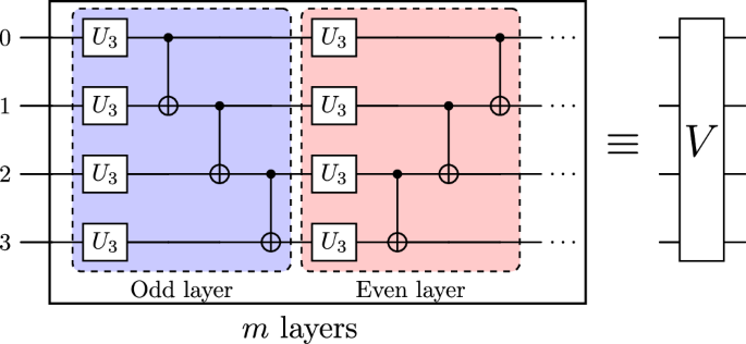
A 4-qubit unitary V is implemented as a parametrized m-layer quantum circuit of alternating odd and even layers. Each universal single-qubit gate U₃ is parametrized by 3 distinct parameters, for a total of n_p = 12m parameters for V. Using our recompilation algorithm, we optimize the circuit over the set of n_p parameters to minimize the trace distance between V and the target unitary U(t) = e^−iHt. In our experiments, we use recompiled circuits with m = 20 layers for a total of 60 CNOT gates.

Full size image

The optimization runs on a regular laptop in a few minutes. The advantages of this optimization method are a drastic reduction in the number of required CNOT gates by 178 and no need for a Trotter approximation, which allows us to run the experiment up to arbitrary long times with good precision, crucial to studying thermalization.

Measurement errors

To mitigate measurement errors, we execute every circuit with a sampling of 1000 shots and correct the outcome using the readout error correction technique that involves matrix inversion through the iterative Bayesian unfolding method⁷³.

Randomized compiling

To mitigate errors arising from the two-qubit gates application, we aim to simplify the noise structure, which allows for the implementation of efficient error mitigation techniques. To do so, we follow the randomized compiling (RC) approach^74,75,76 which enables one to transform any coherent noise affecting CNOT gates into an effective incoherent Pauli noise channel⁷⁷. RC entails generating alternative versions of the quantum circuit of interest, in which every CNOT gate is dressed with Pauli gates acting on individual qubits and drawn randomly from a set of Pauli matrices. These Pauli matrices are drawn in such a way that the dressed CNOT gates are still logically equivalent to an isolated CNOT gate, so that every alternative version of the circuit still implements the same unitary operation. The measured expectation values stemming from each randomly compiled circuit are then averaged, yielding the expectation value that one would have obtained if all CNOT gates were only affected by a purely incoherent noise channel.

In addition to the qubits on which the CNOT gate is applied, a noisy CNOT gate may also lead to coherent errors on neighboring qubits. In our case, this can be formalized by extending the noise channel associated with a given CNOT gate to all qubits in the register. This noise, known as spillover crosstalk noise⁷⁸, can also be made purely incoherent by extending the RC method to neighboring qubits. In addition, since a priori no logical operation is being applied on these other qubits, the RC procedure can be improved by applying extra random π/2 rotations on top of the Pauli matrices, as prescribed in⁴⁵. One can show that by doing this, the effective incoherent noise channel obtained after averaging over crosstalk RC circuits is a combination of a local Pauli noise channel for the active qubits of the CNOT gates, a local depolarizing noise channel acting on the neighboring qubits, and a global depolarizing noise channel acting uniformly on all qubits. In our quantum simulation, we run 100 crosstalk RC circuits for every realization of the quench protocol, and average the read-out observables, effectively realizing the noise channel described above. We have checked for this number of circuits that the crosstalk RC averages has clearly converged to its infinite sampling value. Using our knowledge of the structure of the effective incoherent noise channel acting on our qubits, we now implement an error mitigation strategy.

Removing global depolarizing noise

After performing crosstalk RC, we know that at least a part of the effective noise acting on our circuit takes the form of an N-qubit global depolarizing noise channel. Due to the simplicity of this noise channel, its effects can be mitigated efficiently with a simple fit, as we show here. For a single CNOT gate, the N-qubit global depolarizing noise channel reads⁴⁰:

where ρ the density matrix, f is the fidelity of a CNOT gate and ({mathbb{1}}) the identity matrix of size 2^N. The rightmost term, which models the output of a global depolarizing error occurring, is the maximally mixed state with N qubits. If such an error occurs on any CNOT gate during the execution of the circuit, then the qubits will remain in this state, as it is not affected by the action of subsequent unitary operations. Thus, it is straightforward to generalize Eq. (13) to the case of a circuit with N_CNOT CNOT gates by replacing the fidelity of a single CNOT gate f with a circuit fidelity ({f}^{{N}_{{{{rm{CNOT}}}}}}). Further averaging the quantum simulation data for occupation probabilities over 100 realizations of the quench protocol, we interpret the noisy quantum computer’s output within the model (13), leading to the expression (12) for noisy average occupations. Then, we leverage the errors due to the local Pauli and depolarizing noise channels using zero-noise extrapolation (ZNE).