Dynamical topology of chiral and nonreciprocal state transfers in a non-Hermitian quantum system
Introduction
Geometric phases play a crucial role in classifying gapped quantum systems that are protected by the symmetry of Hamiltonians1,2, often resulting in robust physical properties that are resilient to perturbations. In time-varying cases, if the evolution is sufficiently slow, the system remains in the eigenstate of the instantaneous Hamiltonian, thereby preserving the geometric phases during dynamic processes. This phenomenon, validated in various Hermitian systems3,4,5,6, relies on the preservation of symmetry and adherence to the adiabatic condition. One might expect that this similarly applies to time-varying non-Hermitian systems; However, this expectation does not hold. When encircling the exceptional points (EPs) in a non-Hermitian system, the state deviates from the eigenstate of the instantaneous Hamiltonian regardless of how slowly the system evolves7,8. This deviation is known as dissipation-induced nonadiabatic transitions (DNATs). The occurrence of DNATs disrupts the continuous accumulation of geometric phases on the Riemann surfaces of complex eigenvalues. Consequently, characterizing the topological properties of dynamical non-Hermitian systems remains a significant and unresolved question.
Previous research on encircling EPs in non-Hermitian systems reveals fascinating topological behaviors, which have been experimentally explored in both classical and quantum systems, including microwave/optical setups7,9,10,11,12,13,14, optomechanical oscillators8, acoustic cavities15,16, superconducting circuits17, NV centers18, and cold atoms19. Some of these experiments have demonstrated that in the absence of DNATs, a parameter variation encircling an EP causes two states to switch positions after one cycle and acquires a geometric phase of π after two cycles. With DNATs, however, the geometric phase becomes elusive during dynamic processes. Instead, the vorticity of energy eigenvalues may serve as a type of topological invariant in non-Hermitian systems20,21, but its validity depends on the evolution trajectories remaining on the Riemann surfaces, which is contradicted by the presence of DNATs. The most intriguing topological behaviors in these systems7,8,10, such as chiral state transfers and nonreciprocal mode switching, depend on the occurrence of DNATs. Therefore, it is essential to uncover a profound relationship between DNATs and hidden topological invariants in dynamics. This understanding could help identify the topological structure of non-Hermitian dynamics.
In this work, we experimentally study the topological chiral and nonreciprocal state transfers by dynamically encircling the EPs of both ({{{mathcal{PT}}}}) (parity-time) (([H,{{{mathcal{PT}}}}]=0)) and ({{{mathcal{APT}}}}) (anti-parity-time) symmetric (({H,{{{mathcal{PT}}}}}=0)) Hamiltonians in a trapped-ion system. The outcomes unveil a universal rule for determining the behavior of state transfers associated with chiral and time-reversal symmetries. Chiral state transfers, where encircling an EP in a clockwise or counterclockwise direction results in different final states, are exclusively dictated by the symmetry of the initial effective Hamiltonian in the parallel transported eigenbasis. Nonreciprocal state transfers, where the processes depend on the initial states and the direction of encircling the EP, are dictated by the time derivative of the initial states. We find that these state transfers are robust against substantial external noise introduced during the encircling processes. To reveal the underlying topological mechanism of this robustness, we transform the original Hamiltonian into the case in the parallel transported eigenbasis and define a topological invariant, dynamic vorticity. This dynamic vorticity remains invariant during the encircling process, regardless of whether DNATs occur, and is solely determined by the number of EPs that the trajectories encircle. This reveals that both chiral and nonreciprocal state transfers are protected by dynamic vorticity, which can be considered a universal topological invariant in time-varying non-Hermitian systems. These discoveries validate that topological dynamics can arise from the interplay of dissipation and coherence, opening new avenues to explore the topological properties of open quantum systems.
Results
Dynamically encircling the EPs of ({{{mathcal{PT}}}}) and ({{{mathcal{APT}}}}) symmetric Hamiltonians
The experiments utilize a passive ({{{mathcal{PT}}}})-symmetric system involving a single trapped 171Yb+ ion, building upon the experimental setup (see Methods) described in detail in our previous works22,23,24. The ion is confined and laser-cooled in a linear Paul trap. Then, it is initialized to the hyperfine state (| downarrow left.rightrangle =| F=0,{m}_{F}=0{,}^{2}{S}_{1/2}left.rightrangle) of the ground state by optical pumping. The qubit levels, hyperfine states (| downarrow left.rightrangle) and (| uparrow left.rightrangle =| F=1,{m}_{F}=0{,}^{2}{S}_{1/2}left.rightrangle), are driven by a microwave with a coupling rate J. The dissipation is introduced by resonantly driving a transition from (| uparrow left.rightrangle) to (| F=1,{m}_{F}=0{,}^{2}{P}_{1/2}left.rightrangle) of the excited state, resulting in the spontaneous decay to three ground states (| F=1,{m}_{F}=0,pm 1left.rightrangle) in 2S1/2 with equal probability. Taken the Zeeman sublevels (| F=1,{m}_{F}=pm 1left.rightrangle) in 2S1/2 as an auxiliary state (| aleft.rightrangle), the system is equivalent to a spin-dependent loss from the qubit state (| uparrow left.rightrangle) to state (| aleft.rightrangle) with a rate at 4γ, as the coupling of the qubit to the environment. When the coupling strength of the dissipation beam is significantly lower than the linewidth of the 2P1/2 excited state, the involved energy levels can be approximated to a dissipative two-level system, as illustrated in Fig. 1a. Consequently, a passive ({{{mathcal{PT}}}})-symmetric non-Hermitian Hamiltonian, ({H}_{eff}=J{hat{sigma }}_{x}+igamma {hat{sigma }}_{z}-igamma hat{I}), is derived22,25,26. Here, ({hat{sigma }}_{x}=| downarrow left.rightrangle langle uparrow | +| uparrow rangle leftlangle right.downarrow |), ({hat{sigma }}_{z}=| downarrow left.rightrangle langle downarrow | -| uparrow rangle leftlangle right.uparrow |), and (hat{I}=| downarrow left.rightrangle langle downarrow | +| uparrow rangle leftlangle right.uparrow |). This Hamiltonian can be mapped to a ({{{mathcal{PT}}}})-symmetric Hamiltonian by adding an extra term (igamma hat{I}).

a Schematic diagram of the experimental setup. The blade trap confines a single ion using radio frequency (RF) signals and direct current (DC) voltages applied to two RF and two DC electrode sets. The microwave signal drives the transition between the states (| downarrow left.rightrangle) and (| uparrow left.rightrangle) through the horn. A dissipative beam with π-polarized component, where the electric field (vec{{{{bf{E}}}}}) is parallel to the magnetic field (vec{{{{bf{B}}}}}), excites the ion from (| uparrow left.rightrangle) to the 2P1/2 excited state. The involved energy levels of a 171Yb+ ion include (| F=0,{m}_{F}=0left.rightrangle) and (| F=1,{m}_{F}=0,pm 1left.rightrangle) in the electronic ground state 2S1/2, and (| F=0,{m}_{F}=0left.rightrangle) in the electronic excited state 2P1/2. b Encircling paths in the parameter space (coupling strength J and detuning Δ) and the state evolution trajectories projected onto the eigenvalues’ Riemann sheets, starting in the ({{{mathcal{PT}}}})-symmetric (({{{mathcal{PTS}}}})) regime of the ({{{mathcal{PT}}}}) Hamiltonian. The solid (dashed) trajectory in (b) denotes the clockwise (counterclockwise) evolution of (| {alpha }_{A}(0)left.rightrangle). c Chiral symmetry (depicted by red and blue curves in the left panel) and broken chiral symmetry (depicted by red and green curves in the left panel) serve as mathematical criteria for determining chiral dynamics. In this context, CCW and CW refer to counterclockwise and clockwise, respectively. Time-reversal symmetry (illustrated by red and green curves in the right panel) and broken time-reversal symmetry (illustrated by red and blue curves in the right panel) serve as mathematical criteria for determining nonreciprocal dynamics.
To encircle the EP of the ({{{mathcal{PT}}}}) symmetric Hamiltonian, the driving microwave features time-varying detuning and intensity, resulting in a time-dependent Hamiltonian expressed as (ℏ = 1)
where Δ(t) and J(t) represent the detuning and the coupling rate of the microwave, respectively, and γ denotes the dissipation rate dependent on the laser intensity. The eigenvalues of Eq. (1) are complex numbers given by ({lambda }_{1,2}(t)=pm scriptstylesqrt{J{(t)}^{2}-gamma {(t)}^{2}+igamma (t)Delta (t)+Delta {(t)}^{2}/4}), with the EP occurring at Δ = 0 and J = γ.
The system evolves by varying Δ(t) and J(t), while keeping γ fixed. The real and imaginary components of λ1,2(t) form two intersecting Riemann sheets wrapped around the EP, as shown in Fig. 1b. We drive the qubit through a parameter loop defined by (Delta (t)=rsin [theta (t)+{theta }_{0}]) and (J(t)={J}_{0}+rcos [theta (t)+{theta }_{0}]), where r represents the encircling radius, θ(t) denotes the time-dependent encircling angle, and θ0 = 0 (θ0 = π) determines the starting point in the ({{{mathcal{PT}}}})-symmetric (broken) regime, abbreviated as the ({{{mathcal{PTS}}}}) (({{{mathcal{PTB}}}})) regime. More details regarding the encircling procedure can be found in Methods.
The clockwise and counterclockwise encircling trajectories from the eigenstate (| {alpha }_{A}(0)left.rightrangle) ((| {beta }_{A}(0)left.rightrangle)) are demonstrated in Fig. 2a, c (e and g), where the black lines show the state evolution projected onto the Riemann surfaces. Figure 2b, d (f and h) show the overlap between the instantaneous eigenstate (| alpha (t)left.rightrangle) ((| beta (t)left.rightrangle)) with the evolutionary state (| psi (t)left.rightrangle ={C}_{1}(t)| alpha (t)left.rightrangle, +{C}_{2}(t)| beta (t)left.rightrangle), i.e., (leftlangle {alpha }_{A}(t)| psi (t)rightrangle) ((leftlangle {beta }_{A}(t)| psi (t)rightrangle)). Here, (| alpha (t)left.rightrangle) and (| beta (t)left.rightrangle) represent the eigenstates of time-dependent non-Hermitian Hamiltonian at each moment. When a DNAT occurs, the qubit invariably jumps from the loss sheet (blue) to the gain sheet (red) on the Riemann surface. Such jump is characterized by the crossing between (leftlangle {alpha }_{A}(t)| psi (t)rightrangle) and (leftlangle {beta }_{A}(t)| psi (t)rightrangle) in the cyan shaded region. Its occurrence is measured through quantum state tomography of (| psi (t)left.rightrangle) during these experiments. We also investigate the dynamical encircling with ({{{mathcal{APT}}}}) symmetric Hamiltonians, constructed by sandwiching a passive ({{{mathcal{PT}}}})-symmetric Hamiltonian Heff between two π/2 pulses along the ± Y axis on the Bloch sphere23. The details are provided in Supplementary Note 3.
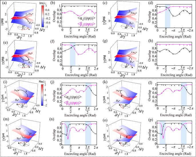
a, c, e, g Clockwise and counterclockwise encircling the EP starting from (| {alpha }_{A}(0)left.rightrangle) and (| {beta }_{A}(0)left.rightrangle) are shown as trajectories 1 to 4. i, k, m, o Similar encircling starting from (| {alpha }_{B}(0)left.rightrangle) and (| {beta }_{B}(0)left.rightrangle) are depicted as trajectories 5 to 8. b, d, f, h Overlaps 〈αA(t)∣ψ(t)〉 and 〈βA(t)∣ψ(t)〉 between the instantaneous eigenstates and the evolutionary state from the ({{{mathcal{PT}}}})-symmetric (({{{mathcal{PTS}}}})) regime. j, l, n, p Overlaps 〈αB(t)∣ψ(t)〉 and 〈βB(t)∣ψ(t)〉 from the ({{{mathcal{PT}}}})-broken (({{{mathcal{PTB}}}})) regime. Nonadiabatic dynamics are shown in the cyan shaded regions. The solid (dashed) box depicts the state evolution trajectories in the visual four-dimensional picture of the eigenspectrum as a function of the detuning Δ and the coupling rate J, with colors on the Riemann sheet representing imaginary (real) values. Circles with error bars represent experimental results obtained from the raw measured data, while lines correspond to numerical simulation results.The error bars are estimated as the standard deviation (1σ) from 5 rounds of quantum state tomography experiments.
Chiral and nonreciprocal state transfers
The analyses of chiral behaviors in state transfer are depicted in the left panel of Fig. 1c. The clockwise evolution of (| {alpha }_{A}(0)left.rightrangle mathop {longrightarrow}limits^{{rm{CW}}} | {beta }_{A}(0)left.rightrangle) (trajectory 1) and the counterclockwise case of (| {alpha }_{A}(0)left.rightrangle mathop {longrightarrow}limits^{{rm{CCW}}} | {alpha }_{A}(0)left.rightrangle) (trajectory 2) exhibit the chiral state transfer, whose evolution trajectories are shown in Fig. 2a–d. Another example of chiral state transfer involves the pair of of (| {beta }_{A}(0)left.rightrangle mathop {longrightarrow}limits^{{rm{CW}}}| {beta }_{A}(0)left.rightrangle) (trajectory 3) and (| {beta }_{A}(0)left.rightrangle mathop {longrightarrow}limits^{{rm{CCW}}}| {alpha }_{A}(0)left.rightrangle) (trajectory 4), as shown in Fig. 2e–h. It is noted that the chiral state transfers are associated with starting points located in the ({{{mathcal{PTS}}}}) regime. The paths in opposite directions experience unequal numbers of DNATs, preserving the chiral symmetry. Conversely, for the starting point in the ({{{mathcal{PTB}}}}) regime, whether starting from (| {alpha }_{B}(0)left.rightrangle) (Fig. 2i–l) or (| {beta }_{B}(0)left.rightrangle) (Fig. 2m–p), both clockwise and counterclockwise paths experience the same number of DNATs, breaking the chiral symmetry.
The right panel of Fig. 1c explains how nonreciprocity is generated due to broken time-reversal symmetry (TRS). Starting from the eigenstates in the ({{{mathcal{PTS}}}}) regime, the forward-time evolution (trajectory 1) and the backward-time evolution (trajectory 4) constitute a pair of reciprocal processes, the same as trajectory 5 and trajectory 6 with the initial eigenstate in the ({{{mathcal{PTB}}}}) regime. For both cases, the same number of DNATs occurs in the forward-time and backward-time paths. On the contrary, if the forward-time and backward-time encircling have different numbers of the DNATs, as seen in trajectories 3 and 4, trajectories 2 and 1, trajectories 7 and 6, and, trajectories 8 and 5, TRS is broken, resulting in nonreciprocal state transfers.
In addition, we systematically investigate the chirality and nonreciprocity with the ({{{mathcal{APT}}}}) Hamiltonian. The emergence of the chiral (nonchiral) behavior in state transfer occurs when the starting point is in the ({{{mathcal{PTB}}}}) (({{{mathcal{PTS}}}})) regime, opposite to the ({{{mathcal{PT}}}})-symmetric Hamiltonian. Regarding the chiral and nonreciprocal properties, we discover a dual relationship between the ({{{mathcal{PT}}}})-Hamiltonian and the ({{{mathcal{APT}}}}) one, where the ({{{mathcal{PTS}}}}) regime of the ({{{mathcal{APT}}}}) Hamiltonian is equivalent to the ({{{mathcal{PTB}}}}) regime of the ({{{mathcal{PT}}}}) Hamiltonian, and vice versa (See Supplementary Note 3).
Based on the aforementioned observations, we ascertain that the unequal numbers of DNATs appearing in a pair of encircling paths result in chiral and nonreciprocal state transfers. The crucial role of DNATs stems from the dynamical phase accumulated as the parameters of the Hamiltonian evolve adiabatically27,28. The evolutionary state is expressed as (| {psi }_{n}(t)left.rightrangle) =({e}^{-frac{i}{hslash }int{E}_{n}({{{bf{R}}}}({t}^{{prime} }))d{t}^{{prime} }}cdot {e}^{igamma (t)}| n({{{bf{R}}}}(t))left.rightrangle), where ({e}^{-frac{i}{hslash }int{E}_{n}({{{bf{R}}}}({t}^{{prime} }))d{t}^{{prime} }}) is dynamical phase term, eiγ(t) is geometric phase term, and (| n({{{bf{R}}}}(t))left.rightrangle) is instantaneous eigenstate state of Hamiltonian. When the state evolves on the loss sheet, the dynamical phase contributes a decaying factor. Consequently, the state evolving on the loss sheet will transition to the gain sheet, whereas the state on the gain sheet will remain unaffected.
Classification of nonadiabatic transitions
We have developed a quantitative approach to examine the dependence of chirality and nonreciprocity on the adiabaticity of the encircling process. In this method, the chiral and nonreciprocal behaviors are characterized by the the fidelity of state transfer during one encircling of the EP, defined as the squared overlap between the final state ψ(T) and the initial state. The adiabaticity of the encircling is quantified by τcrit= max(left(frac{1}{{lambda }_{1}(t)-{lambda }_{2}(t)}right)). In the experiments, the fidelities of state transfer (| {alpha }_{A}(0)left.rightrangle mathop {longrightarrow}limits^{{rm{CW}}}| {beta }_{A}(0)left.rightrangle) (trajectory 1), i.e., ∣〈αA(0)∣ψ(T)〉∣2 and ∣〈βA(0)∣ψ(T)〉∣2, are studied with various encircling periods and radii, as shown in Fig. 3. These results demonstrate the dependence of chirality and nonreciprocity on the adiabaticity of the encircling process.

a, b The ratio of the critical time to the evolution time, τcrit/T, as a function of the encircling period and radius. The black curves are contour lines. c, d Fidelity changes in state transfer with varying periods and radii. The contour map and solid lines denote the simulation results, while the circles with error bars represent the experimental results obtained from the raw measured data. e, f Overlaps 〈αA(t)∣ψ(t)〉 (solid line) and 〈βA(t)∣ψ(t)〉 (dash line) with varying periods for the initial state (e) (| {alpha }_{A}(0)left.rightrangle) and (f) (| {beta }_{A}(0)left.rightrangle), respectively. The blue, red, and black circles correspond to T = 16.67 μs, 100 μs, and 250 μs, matching the vertical lines in (a). g—h Overlaps with varying radii for the initial state (g) (| {alpha }_{A}(0)left.rightrangle) and (h) (| {beta }_{A}(0)left.rightrangle), respectively. The blue, red, and black squares correspond to r = 0.003 MHz, 0.008 MHz, and 0.03 MHz, matching the vertical lines in (b). The error bars are estimated as the standard deviation (1σ) from 5 rounds of quantum state tomography experiments.
The results for various periods are shown in Fig. 3a. τcrit = 11.8 μs for all selected periods. For an encircling period T = 250 μs ≫ τcrit that satisfies the adiabatic criteria, the fidelity of state transfer ({langle {beta }_{A}(0)| psi (T)rangle }^{2}) is nearly unity, representing almost perfect state swaps of (| {alpha }_{A}(0)left.rightrangle) and (| {beta }_{A}(0)left.rightrangle). When the encircling period reduces, the deviations from the ideal fidelities get larger and larger, as shown in shown in the olive curve of the side plane in Fig. 3c, d. For example, for T = 100 μs, 〈βA(0)∣ψ(T)〉 becomes smaller than the unity, indicating that the final state fails to fully reach (| {beta }_{A}(0)left.rightrangle). This decay of state overlap is more obvious for T = 16.67 μs. Such deviation from (| {beta }_{A}(0)left.rightrangle) leads to the breakdown of the chiral and nonreciprocal state transfers.
The results for various radii are also depicted in the dark yellow curve on the side plane in Fig. 3c, d, showing that chiral and nonreciprocal behaviors are primarily observed at larger radii. For r = 0.03 MHz, the fidelity of ({langle {beta }_{A}(0)| psi (T)rangle }^{2}) approaches unity. However, as the radius decreases, τcrit/T < 0.1, resulting in a significant deviation from the predictions of the adiabatic theorem. The state transfer for the ({{{mathcal{APT}}}})-symmetric Hamiltonian, with varying periods and radii, can be found in Supplementary Note 3.
Here, we observe DNATs during the adiabatic evolution of system parameters, which are distinctly different from the conventional speed-induced nonadiabatic transitions (SNATs) where the evolution does not satisfy the adiabatic theorem. In Fig. 3e, as the period reduces from T = 250 μs to T = 16.67 μs, we observe a crossing of 〈αA(t)∣ψ(t)〉 and 〈βA(t)∣ψ(t)〉 (for T = 16.67 μs blue curves), indicating the occurrence of a SNAT. Additionally, reducing the encircling period deviates the path from the prediction dictated by the adiabatic theorem, as demonstrated by the different crossings in Fig. 3f. The new crossing of 〈αA(t)∣ψ(t)〉 and 〈βA(t)∣ψ(t)〉 does not appear due to the dominant DNAT. Notably, decreasing the encircling radius does not generate SNATs but only decreases the fidelity of the DNAT, as shown in Fig. 3g, h.
Robustness of the state transfer
We experimentally verify the topological robustness of state transfers using ({{{mathcal{PT}}}}) and ({{{mathcal{APT}}}})-symmetric Hamiltonians against the physical noises in a dissipative trapped-ion qubit. For the ({{{mathcal{PT}}}}) Hamiltonian, we introduce noises into the detuning and the coupling rate along the encircling path
where the encircling radius r = 0.03 MHz, the dissipation rate γ = 0.06 MHz, and κ(t) represents the noise in the encircling process. κ(t) ∈ [ − ir, ir] is generated by pseudorandom real number, where ir is defined as the intensity of the noise.
Figure 4 illustrates the final state outcomes of the encircling process, showing that it remains unaffected by random noise, regardless of the noise intensity. Figure 4a–d (e–h) displays the experimental results for the ({{{mathcal{PT}}}})-symmetric (broken) regime. We find that chiral and nonreciprocal quantum state transfers exhibit robustness against such noise, provided the adiabatic encircling condition is satisfied. Even in the adiabatic limit of evolution, this robustness persists near the EP because the external noise fails to eliminate the degeneracy at the EP. We have also experimentally verified the topological robustness of the quantum state transfer with the ({{{mathcal{APT}}}})-symmetric Hamiltonian, as detailed in Supplementary Note 3. In both cases, the experimental data match pretty well with the theoretically predicted values, even under varying noise intensities. This validation confirms the robustness of topological state transfer with ({{{mathcal{APT}}}})-symmetric Hamiltonians.

a, c, e, g The color maps show the overlap between the instantaneous eigenstate and the evolutionary state under varying noise intensities. b, d, f, h Experimental results of robustness under different noise intensities, corresponding to the three dashed lines in (a, c, e, g). Dots with error bars are experimental results obtained from the raw measured data and solid lines are the simulation predictions. Insets in (b, f) display clockwise encircling trajectories in the two-dimensional parameter space of detuning Δ and coupling rate J, with random noise intensities ir = 0 (black), 0.3 (red), and 0.5 (blue), respectively. In (a–d), the encircling starts from point A in the ({{{mathcal{PT}}}})-symmetric (({{{mathcal{PTS}}}})) regime, while in (e–h), it starts from point B in the ({{{mathcal{PT}}}})-broken (({{{mathcal{PTB}}}})) regime. The error bars are estimated as the standard deviation (1σ) from 5 rounds of quantum state tomography experiments.
Discussions
In this study, we have observed chiral (nonreciprocal) quantum dynamics in a trapped-ion qubit, wherein the EPs of both ({{{mathcal{PT}}}})-symmetric and ({{{mathcal{APT}}}})-symmetric Hamiltonians are dynamically encircled. These dynamics are rooted in the unique topological structure of intersecting Riemann sheets around the EP. During adiabatic state transfers, this structure leads to the swapping of two eigenstates after one cycle and the acquisition of a geometric phase of π after two cycles9,15. The topological invariant of the adiabatic process is characterized by this geometric phase, providing the protection against perturbations. For nonadiabatic processes, it is usually believed that the nonadiabaticity would cause the evolution to deviate from the eigenstates of the instantaneous Hamiltonian, and consequently undermine topological protection from the Riemann surface. However, previous experiments have confirmed the robust state transfer not only for adiabatic processes, but also existing in ones involving dissipation-induced nonadiabatic transitions14,16,29,30. This raises one critical question: is there a topological invariant to elucidate the robust state transfers in nonadiabatic processes, which could unveil the topological structure of DNATs. Addressing this question is crucial for fully understanding chiral and nonreciprocal state transfers in non-Hermitian systems. To date, this question remains unexplored.
Based on the above results, we address this question by providing a topological invariant that we dub as “dynamic vorticity” for characterizing topological protections involving DNATs. Previously, the vorticity, also known as the spectral or eigenvalue winding number20,21,31,32, is defined as ({{{mathcal{V}}}}=-frac{1}{2pi }{oint }_{Gamma }{nabla }_{k}{{{rm{Arg}}}}[{E}_{m}(k)-{E}_{n}(k)]cdot dk). Here eigenvalues Em(k) and En(k) are varied with momentum k (k ∈ [0, 2π]) in the Brillouin zone and the indices m and n represent different band structures. Noted that, in this scenario, although eigenvalues parametrically change along the close loop Γ in the momentum space, there are no dynamics or nonadiabatic transitions driven by time-dependent Hamiltonian. Under this condition, the vorticity presents the topological structure of a static Hamiltonian. In our case, we deal with the time-dependent Hamiltonian, which generates real time dynamics, including nonadiabatic transition.
To effectively explain the robustness of the chiral and nonreciprocal dynamics that we observed experimentally. We find that the vorticity concept can be extended to the time-dependent Hamiltonian. To include the dynamics, we adopt the parallel transported eigenbasis33, giving
the nonadiabatic transition process is reflected in the off-diagonal term of Eq. (3) since (f(t)=(J(dot{Delta }/2+idot{gamma })-dot{J}(Delta /2+igamma ))/2i{lambda }^{2}) includes the time derivatives of both the coupling J and the detuing Δ, as seen from Eq. (15) (Details in Methods). Then, the dynamic vorticity is given by
where ({widetilde{E}}_{pm }(theta =omega t)) are dynamically varied with encircling angle θ(θ ∈ [0, 2π]) in the parameter space. The dynamic vorticity associates with the energy dispersion of ({widetilde{H}}_{eff}(t)), which characterizes the topology of dynamics of encircling the EP. The validity of ({{{{mathcal{V}}}}}_{{{{mathcal{D}}}}}) lies in the fact that, in the parallel transported basis, nonadiabatic transitions will not cause the deviations of the instantaneous state from the Riemann surfaces. Consequently, the system’s evolution consistently remains in the eigenstate of ({widetilde{H}}_{eff}(t)). Therefore, ({{{{mathcal{V}}}}}_{{{{mathcal{D}}}}}) is a universal topological invariant near the EP not only for adiabatic dynamics, but also for nonadiabatic ones, which can be treated as the winding number of the complex-energy bands, as detailed in Supplementary Note 2. It is also noted that the definition and form of Eq. (4) apply to both ({{{mathcal{PT}}}})-symmetric and passive ({{{mathcal{PT}}}})-symmetric Hamiltonians, since introducing an extra diagonal term does not alter the basic topology of the dynamics.
For the topologically protected chiral and nonreciprocal state transfers in Fig. 2, we find that ({{{{mathcal{V}}}}}_{{{{mathcal{D}}}}}=pm 1/2), i.e., − 1/2 for trajectory 1 and 1/2 for trajectory 2. Meanwhile, for state transfers that do not encircle an EP, Refs. 10,13 also show that such processes remain topologically robust, in which our numerical simulation gives ({{{{mathcal{V}}}}}_{{{{mathcal{D}}}}}=0). Therefore, we conclude that ({{{{mathcal{V}}}}}_{{{{mathcal{D}}}}}=0,pm 1/2) characterize topological state transfers, where the sign ± depends on the orientation of the encircling curve.
Another advantage of using the parallel transported eigenbasis is that the effective Hamiltonian in this basis can be used to determine the occurrence of chiral behavior. If the initial effective Hamiltonian satisfies ({{widetilde{H}}_{eff}(0),{{{mathcal{CPT}}}}}=0), where we define the chiral operator ({{{mathcal{S}}}}={{{mathcal{CPT}}}}), our experimental results indicate a pair of encircling dynamics have the chiral symmetry (i.e., trajectories 1 and 2 in Fig. 2 have different final states). Here, parity operator ({{{mathcal{P}}}}={sigma }_{x}), ({{{mathcal{C}}}}={sigma }_{z}), and time-reversal operator ({{{mathcal{T}}}}) represents the conjugate operator. Conversely, if ({{widetilde{H}}_{eff}(0),{{{mathcal{CPT}}}}}ne 0), the dynamics breaks the chiral symmetry (i.e., trajectories 5 and 6 in Fig. 2 have the same final states). Note that ({{{mathcal{S}}}}={{{mathcal{CPT}}}}) instead of ({{{mathcal{S}}}}={{{mathcal{CT}}}}) in the Hermitian case2,34 due to non-Hermiticity35. We also find that the nonreciprocal behavior depends on the initial density matrix ρ(0). The positive (negative) value of ({{{rm{Tr}}}}({sigma }_{z}rho (0))) corresponds to the preservation (breakdown) of TRS for a pair of the forward-time and backforward-time encircling processes. When ({{{rm{Tr}}}}({sigma }_{z}rho (0))=0), if (d[{{{rm{Tr}}}}({sigma }_{z}rho (t))]/dt{| }_{t = 0}, > , 0), the processes preserve the TRS (i.e., trajectories 1 and 4). Otherwise, they exhibit the nonreciprocal behavior. Therefore, we conclude that the chiral and nonreciprocal dynamics are dictated by the symmetry of the effective Hamiltonian ({widetilde{H}}_{eff}(0)) and the initial state.
It is worth mentioning that the dynamic vorticity is not suitable for speed-induced nonadiabatic processes, where the evolution period is shorter than the critical time stipulated by the adiabatic theorem. Our results in Fig. 3 show that the occurrence of SNATs disrupts the chiral and nonreciprocal dynamics due to the nonadiabaticity of the Landau-Zener tunneling from an eigenstate to another at the avoided-crossing.
Methods
Experimental setup
A single 171Yb+ ion is confined in a homemade blade trap by applying radio frequency (RF) signals and direct current (DC) voltages to two RF electrodes and two sets of DC electrodes, respectively, are shown in Fig. 1a. The system includes a pair of Helmholtz coils that generate a magnetic field (vec{{{{bf{B}}}}}) of approximately 6 Gauss, which not only lifts the degeneracy of the three magnetic levels but also prevents the ion from being pumped into a coherent dark state. The microwave signal used for driving the qubit rotation consists of a 12.61 GHz signal from standard RF source (Rohde and Schwarz, SMA 100B) and a 31.25 MHz signal from an arbitrary waveform generator (AWG, Spectrum Instrumentation). The dissipative beam only contains the π polarization component, with its electric field (vec{{{{bf{E}}}}}) parallel to the magnetic field (vec{{{{bf{B}}}}}), and is used to excite the ion from (| uparrow left.rightrangle) to the 2P1/2 excited state. This excitation leads to spontaneous decay to three magnetic levels (| F=1,{m}_{F}=0,pm 1left.rightrangle) in the 2S1/2 ground state with equal probability. The decay to (| F=1,{m}_{F}=pm 1left.rightrangle) can be considered as equivalent loss of the qubit, resulting in a nonunitary evolution of the two-level system.
Encircling method
The dynamically encircling of the EP is realized by using the time-dependent detuning (Delta (t)=rsin [theta (t)+{theta }_{0}]) (in MHz) and the time-dependent coupling rate (J(t)={J}_{0}+rcos [theta (t)+{theta }_{0}]) (in MHz), while keeping the dissipation rate fixed18. Here, r is the encircling radius, θ(t) = ωt is the encircling angle, and ω is the angular speed of encircling whose sign determines the encircling direction (“+” for clockwise encircling and “-” for counterclockwise encircling). The parameter θ0 = 0 (θ0 = π) indicates that the starting point lies at the ({{{mathcal{PTS}}}}) (({{{mathcal{PTB}}}})) regime.
The evolutionary state at each time step, i.e. (| psi (t)left.rightrangle ={C}_{1}(t)| alpha (t)left.rightrangle +{C}_{2}(t)| beta (t)left.rightrangle) is the coherent superposition of the eigenstates (| alpha (t)left.rightrangle) and (| beta (t)left.rightrangle). The coefficients C1(t) and C2(t) are probability amplitudes of the (| alpha (t)left.rightrangle) and (| beta (t)left.rightrangle), respectively, as demonstrated in Supplementary Note 1. The trajectory of the encircling, i.e., (∣C1(t)∣2λ1 + ∣C2(t)∣2λ2)/(∣C1(t)∣2 + ∣C2(t)∣2) is derived, where the sudden transitions between (| alpha (t)left.rightrangle) and (| beta (t)left.rightrangle) can be analyzed through the adiabatic multipliers36,37. With the derived trajectory, the state evolution is projected onto the complex Riemann sheets of the eigenvalues, shown as the black line in Fig. 1b of the main text.
The presence of spin-dependent loss causes the qubit population to exponentially decay in a sinusoidal manner for small γ/J ratios22,23,38, leading to an extremely low state population that is challenging to detect experimentally. In response to this challenge, we employ a piecewise strategy. Encircling starts at t = 0 and ends at (T=frac{15}{gamma }). Throughout the encircling process, the dissipation rate remains constant at γ = 0.06 MHz, the angular speed is maintained at (omega =pm frac{2pi }{T}), and the radius is fixed at r = 0.03 MHz (unless specified otherwise in subsequent experiments).
The entire encircling path, with a period of T = 2π/ω, is divided into N segments. In each of the N segments (1 ≤ n ≤ N), the qubit state is prepared to evolve for tn = (n − 1)T/N time according to theoretical prediction. Then, it continues to evolve for t = T/N under the Hamiltonian H(tn). With this scheme, we map out the whole encircling process by quantum state tomography of (| psi (t)left.rightrangle), which is carried out at the end point of each segment. The overlap (i.e., the inner product) of the measured evolutionary state (| psi (t)left.rightrangle) and the instantaneous eigenstates (| {alpha }_{A}(t)left.rightrangle) (or (| {beta }_{A}(t)left.rightrangle)) of the time-varying Hamiltonian Heff(t) is used to evaluate whether the measured state (| psi (t)left.rightrangle) matches with the theoretical calculation.
We adjust the size of N to verify the effectiveness of the piecewise strategy as shown in Fig. 5, where J = 0.06 MHz and ω = 2π × 4 rad ms−1, respectively. The encircling starts from (| {alpha }_{A}(0)left.rightrangle), and N varies with 10 (black squares), 20 (red squares), 30 (green squares), 50 (blue squares), 80 (cyan squares) and 100 (magenta squares). The numerical calculation has a 5% uncertainty (orange error band) in the density matrix of the measured evolutionary state (| psi (t)left.rightrangle), accounting for the fluctuations of the dissipation strength and the coupling strength. The nonzero overlap between (| {beta }_{A}(0)left.rightrangle) and (| psi (0)left.rightrangle) is due to the nonorthogonality of the two eigenstates of Heff(0). The experimental results for N = 100 agree well with the numerical simulation, while the others do not, proving the validness of the proposed scheme for N ≥ 100. Therefore, we choose N = 100 in the following experiments to investigate the dynamics of the encircling.

a The overlap between the evolutionary state (| psi (t)left.rightrangle) and instantaneous eigenstate (| {alpha }_{A}(t)left.rightrangle). b The overlap between the evolutionary state (| psi (t)left.rightrangle) and instantaneous eigenstate (| {beta }_{A}(t)left.rightrangle). Experimental results for N = 10, 20, 30, 50, 80, and 100 are represented by black, red, green, blue, cyan, and magenta dots, respectively. The yellow shaded region represents the numerical calculation with 5% uncertainty in the density matrix of the measured state (| psi (t)left.rightrangle), accounting for fluctuations in the dissipation strength and the coupling strength.The error bars are estimated as the standard deviation (1σ) from 5 rounds of quantum state tomography experiments.
Mapping nonadiabatic transition amplitudes
The nonadiabatic transitions that occur during the encircling of the EP can be attributed to the Stokes phenomenon of asymptotics39,40 or stability loss delay28,41. Here, we analyze DNATs observed in our experiment using the method of parallel transported basis28. The state evolution for a passive ({{{mathcal{PT}}}}) Hamiltonian is determined by (ℏ=1)
where (leftvert psi (t)rightrangle ={C}_{1}(t)leftvert alpha (t)rightrangle +{C}_{2}(t)leftvert beta (t)rightrangle ) and ({H}_{eff}=left(begin{array}{cc}Delta /2&J\ J&-Delta /2-2igamma end{array}right)).
The eigenvalues of Heff are ({widetilde{lambda }}_{pm }=-igamma pm scriptstylesqrt{{(Delta /2+igamma )}^{2}+{J}^{2}}=-igamma pm lambda), where λ is the eigenvalue of the ({{{mathcal{PT}}}})-symmetric Hamiltonian ({H}_{{{{mathcal{PT}}}}}) with detuning. The normalized eigenstates of Heff are
which can be expressed as the parallel transported eigenbasis
where
Then, we use (leftvert alpha rightrangle =Tleft({{1}atop{0}}right)), (leftvert beta rightrangle =Tleft({{1}atop{0}}right)) to represent the parallel transported eigenbasis of Eq. (7). The rotation matrix (T=left(begin{array}{cc}cos (theta /2)&-sin (theta /2)\ sin (theta /2)&cos (theta /2)end{array}right)), where TT⊤ = T⊤T = 1.
Now (| psi (t)left.rightrangle =T| {psi }^{{prime} }(t)left.rightrangle), where (| {psi }^{{prime} }(t)left.rightrangle ={C}_{1}(t)left({{1}atop{0}}right)+{C}_{2}(t)left({{1}atop{0}}right)= left({{{C}_{1}(t)}atop{{C}_{2}(t)}}right)). Substituting the (| psi (t)left.rightrangle =T| {psi }^{{prime} }(t)left.rightrangle) into Eq. (5), we obtain
We consider the evolution ({U}^{{prime} }(t)) defined by (| {psi }^{{prime} }(t)left.rightrangle ={U}^{{prime} }(t)| {psi }^{{prime} }(0)left.rightrangle). Eq. (9) can be rewritten as (frac{partial }{partial t}(T{U}^{{prime} }(t))=-i{H}_{eff}(T{U}^{{prime} }(t))), which is simplified as
Multiplying T⊤ to the left of both sides in Eq. (10), we obtain
where
Then,
Substituting Eq. (13) into Eq. (11), we obtain
where
Expressing ({U}^{{prime} }(t)) in matrix form ({U}^{{prime} }(t)=left(begin{array}{cc}{U}_{alpha alpha }^{{prime} }(t)&{U}_{alpha beta }^{{prime} }(t)\ {U}_{beta alpha }^{{prime} }(t)&{U}_{beta beta }^{{prime} }(t)\ end{array}right)). Its differential form can be described as
If the initial state is (| alpha (0)left.rightrangle), meaning C1(0) = 1, C2(0) = 0, then the final state (| {psi }^{{prime} }(t)left.rightrangle ={U}^{{prime} }(t)left(begin{array}{c}1\ 0end{array}right)=left(begin{array}{c}{U}_{alpha alpha }^{{prime} }(t)\ {U}_{beta alpha }^{{prime} }(t)end{array}right)=left(begin{array}{c}{C}_{1}(t)\ {C}_{2}(t)end{array}right)). This implies that ({U}_{alpha alpha }^{{prime} }(t)) and ({U}_{beta alpha }^{{prime} }(t)) serve as the amplitudes of the corresponding eigenstates. Therefore, the relative nonadiabatic transition amplitudes can be defined as ({R}_{1}(t)=frac{{U}_{beta alpha }^{{prime} }(t)}{{U}_{alpha alpha }^{{prime} }(t)}). Initially set at R1(0) = 0, if the evolution remains adiabatic, R1(t) < 1. However, in the case of the nonadiabatic transition, where two eigenstates exchange position, R1(t) > 1. The same applies to the initial state (| beta left.rightrangle), where C1(0) = 0 and C2(0) = 1. In this case, ({R}_{2}(t)=frac{{U}_{alpha beta }^{{prime} }(t)}{{U}_{beta beta }^{{prime} }(t)}) is employed to indicate the occurrence of nonadiabatic transitions. Utilizing Eq. (16), we derive the differential equations governing the relative nonadiabatic transition amplitudes.
We can also calculate R1(t) and R2(t) by measuring C1(t) and C2(t), giving ({R}_{1}(t)=frac{{C}_{2}(t)}{{C}_{1}(t)}) and ({R}_{2}(t)=frac{{C}_{1}(t)}{{C}_{2}(t)}). For clockwise encircling from (| {alpha }_{A}(0)left.rightrangle) in Fig. 6a, ({R}_{1}(t)=frac{{C}_{2}(t)}{{C}_{1}(t)}, < , 1) in the whole period, indicating C1(t) and C2(t) do not cross, so no DNAT occurs. Similarly, in Fig. 6b, ({R}_{1}(t)=frac{{C}_{2}(t)}{{C}_{1}(t)}) evolves from R1(t) < 1 to R1(t) > 1, indicating C1(t) and C2(t) cross, hence a DNAT occurs. Both the theoretical and experimental results for ({{{mathcal{PTS}}}}) and ({{{mathcal{PTB}}}}) regimes are shown in Fig. 6.

a–d Encircling starting from the ({{{mathcal{PT}}}})-symmetric regime. Clockwise and counterclockwise encircling with the initial state (| {alpha }_{A}(0)left.rightrangle) in (a, b). Similar encircling with (| {beta }_{A}(0)left.rightrangle) in (c, d). e–h Encircling starting from the ({{{mathcal{PT}}}})-broken regime. Clockwise and counterclockwise encircling with the initial state (| {alpha }_{B}(0)left.rightrangle) in (e, f). Similar encircling with (| {beta }_{B}(0)left.rightrangle) in (g, h). The color maps for the time-dependent nonadiabatic transition amplitude when changing the encircling period. The cyan circles with error bars represent experimental results obtained from the raw measured data. Solid and dashed lines on the side plane correspond to the theoretical calculation from Eq. (17) and the numerical simulation from C1(t) and C2(t), where the encircling period T = 250 μs. The error bars are estimated as the standard deviation (1σ) from 5 rounds of quantum state tomography experiments.
Responses